AerGOM, an improved algorithm for stratospheric aerosol extinction retrieval from GOMOS observations – Part 2: Intercomparisons

(1)

www.atmos-meas-tech.net/9/4701/2016/ doi:10.5194/amt-9-4701-2016

AerGOM, an improved algorithm for stratospheric aerosol

extinction retrieval from GOMOS observations –

Part 2: Intercomparisons

Charles Étienne Robert1, Christine Bingen1, Filip Vanhellemont1, Nina Mateshvili1, Emmanuel Dekemper1, Cédric Tétard1, Didier Fussen1, Adam Bourassa2, and Claus Zehner3

1_{Institut d’Aéronomie Spatiale de Belgique, Brussels, Belgium}

2_{Institute of Space and Atmospheric Studies, University of Saskatchewan, Saskatoon, Canada} 3_{ESA European Space Research Institute, Frascati, Italy}

Correspondence to:Charles Étienne Robert ([email protected])

Received: 1 February 2016 – Published in Atmos. Meas. Tech. Discuss.: 16 March 2016 Revised: 5 August 2016 – Accepted: 8 August 2016 – Published: 21 September 2016

Abstract.AerGOM is a retrieval algorithm developed for the GOMOS instrument onboard Envisat as an alternative to the operational retrieval (IPF). AerGOM enhances the quality of the stratospheric aerosol extinction retrieval due to the ex-tension of the spectral range used, refines the aerosol spec-tral parameterization, the simultaneous inversion of all atmo-spheric species as well as an improvement of the Rayleigh scattering correction. The retrieval algorithm allows for a good characterization of the stratospheric aerosol extinction for a wide range of wavelengths.

In this work, we present the results of stratospheric aerosol extinction comparisons between AerGOM and vari-ous spaceborne instruments (SAGE II, SAGE III, POAM III, ACE-MAESTRO and OSIRIS) for different wavelengths. The aerosol extinction intercomparisons forλ <700 nm and above 20 km show agreements with SAGE II version 7 and SAGE III version 4.0 within±15 % and±45 %, respectively. There is a strong positive bias below 20 km at λ <700 nm, which suggests that cirrus clouds at these altitudes have a large impact on the extinction values. Comparisons per-formed with GOMOS IPF v6.01 alongside AerGOM show that at short wavelengths and altitudes below 20 km, IPF re-trievals are more accurate when evaluated against SAGE II and SAGE III but are much less precise than AerGOM. A modified aerosol spectral parameterization can improve Aer-GOM in this spectral and altitude range and leads to results that have an accuracy similar to IPF retrievals. Comparisons of AerGOM aerosol extinction coefficients with OSIRIS and

SAGE III measurements at wavelengths larger than 700 nm show a very large negative bias at altitudes above 25 km. Therefore, the use of AerGOM aerosol extinction data is not recommended forλ >700 nm.

Due to the unique observational technique of GOMOS, some of the results appear to be dependent on the star oc-cultation parameters such as star apparent temperature and magnitude, solar zenith angle and latitude of observation. A systematic analysis is carried out to identify biases in the dataset, using the various spaceborne instruments as refer-ences. The quality of the aerosol retrieval is mainly influ-enced by the star magnitude, as well as star temperature to a lesser degree. To ensure good-quality profiles, we suggest to select occultations performed with star magnitudeM <2.5 and star temperatureT >6×103K. Stray-light contamina-tion is negligible for extinccontamina-tion coefficients below 700 nm us-ing occultations performed with a solar zenith angle>110◦ but becomes important at larger wavelengths. Comparison of AerGOM results in the tropics shows an enhanced bias below 20 km that seem to confirm cirrus clouds as its cause. There are also differences between mid-latitude and tropical obser-vations that cannot yet be explained, with a bias difference of up to 25 %.

(2)

1 Introduction

Stratospheric aerosols are an important part of the Earth sys-tem due to their impact on the planet’s radiative balance and the crucial role they play in heterogeneous chemistry (Solomon et al., 2011). They can be produced either via binary homogeneous nucleation of H2SO4 and H2O close to the tropical tropopause (so-called background aerosols) or during volcanic eruptions, and form the so-called Junge layer, extending from the tropopause to approximately 35 km (Junge et al., 1961).

In order to better understand their behaviour and evolu-tion, it is critical to observe these particles globally and over an extended period of time. Various techniques have been employed to retrieve stratospheric aerosols such as solar oc-cultation (e.g. Kent and McCormick, 1984; Thomason et al., 2008; Randall et al., 2001; Thomason et al., 2010; Sioris et al., 2010), balloon-borne measurements (Hofmann et al., 1975; Renard et al., 2002; Deshler et al., 2003), satellite limb sounding (Taha et al., 2011; Bourassa et al., 2007), ground-based lidar (DeFoor et al., 2012; Jäger, 2005), and twilight brightness variation (Mateshvili, 2005).

Another measurement technique, stellar occultation from space, was utilized by the Global Ozone Monitoring by Oc-cultation of Stars (GOMOS). This instrument collected trans-mission spectra from the Earth’s limb in the UV–Vis–NIR, allowing the retrieval of atmospheric profiles from various species, such as O3, NO2, NO3, as well as aerosol extinc-tion profiles (Kyrölä et al., 2004; Bertaux et al., 2010). These species are currently retrieved by the latest GOMOS opera-tional data processing algorithm (Kyrölä et al., 2012), here-after referred to as IPF v6.01.

Recently, a new stratospheric aerosol retrieval algorithm called AerGOM, extensively covered in a companion paper (Vanhellemont et al., 2016), has been applied to the GO-MOS transmission data in order to obtain improved strato-spheric aerosol profiles. AerGOM is currently the main al-gorithm used to produce the stratospheric aerosol dataset for the Aerosol Climate Change Initiative (Aerosol_CCI), an ESA project focusing on both tropospheric and stratospheric aerosols (Holzer-Popp et al., 2013).

The purpose of this paper is to assess the agreement and discrepancy between AerGOM stratospheric extinction measurements at different wavelengths and those of vari-ous spaceborne instruments that observed the stratosphere in the same spectral range during the Envisat mission, namely SAGE II, SAGE III, POAM III, MAESTRO and OSIRIS. Beside the general comparison between AerGOM and other instruments, the influence of various stellar occultation pa-rameters such as star magnitude and temperature, solar zenith angle as well as the spatio-temporal variability is studied.

2 The GOMOS instrument

GOMOS was on-board the successful ESA Environmental Satellite (Envisat) mission. Envisat payloads gathered infor-mation about the state of the Earth’s atmosphere from shortly after its launch in March 2002 until communication was lost with the satellite in April 2012. The GOMOS instrument functioned almost continuously during its lifetime, except in 2005 when problems with the instrument forced the ground segment team to switch to the redundant measurement sys-tem due to errors with the scanning mirrors, impacting mea-surements during several months (ESA, 2007).

The instrument measured the light transmission from up to 300 stars through the Earth’s atmosphere using four spec-trometers covering the following spectral regions: 248–371, 387–693, 750–776 and 915–956 nm. The vertical sampling ranges from 200 m to 1.7 km, depending on the obliquity and the tangent altitude of the observation.

The starlight transmission is not only affected by scatter-ing and absorption but also modified by refractive effects such as chromatic refraction and refractive dilution. More problematic for the analysis of the transmission spectra how-ever is scintillation, i.e. random fluctuations in the measured intensity of stellar light caused by refractive irregularities due to atmospheric instability. Two fast photometers measuring in the blue (473–527 nm) and the red (646–698 nm) part of the visible spectrum were used for the scintillation correc-tion and also provided high-resolucorrec-tion temperature profiles (Sofieva et al., 2009).

Beyond these issues, the uncertainty of the retrieval is largely determined by the temperature and magnitude of the observed star. Even bright stars are point sources of low-intensity compared with the sun. Hence, profiles obtained from stellar occultations have larger uncertainties compared with solar occultation measurements. However, this draw-back is compensated by the fact that stars are abundant in the sky: 30–40 occultations per orbit have been typically per-formed (compared with the 2 occultations available in the case of solar occultation), although this number decreased to 20–30 occultations per orbit after the instrument malfunc-tion in 2005. The retrieval of species using stellar occultamalfunc-tion is possible in both bright and dark limb, but in the case of bright limb geometry, the weakness of the signal compared to the ambient light makes the retrieval even more challeng-ing. At this stage, bright limb measurements are not used for the retrieval of stratospheric aerosol extinctions.

(3)

sec-ond step is the spatial inversion, where the slant path columns for each species are inverted to local concentration/extinction profiles. The spatial inversion uses the Tikhonov altitude smoothing technique (Twomey, 1996; Rodgers, 2000) to remove the residual scintillation perturbations in measure-ments.

The current choice of the Tikhonov parameters leads to the removal of all strong oscillations, at the cost of the vertical resolution, chosen as 4 km (Vanhellemont et al., 2010).

The specification of the aerosol scattering cross section is difficult since the aerosol content may be very different depending on the state of the atmosphere and the nature of the dominant aerosol mode (background, volcanic, etc.). The current (v6.01) spectral inversion assumes that the strato-spheric aerosol extinction obeys a quadratic polynomial as a function of wavelength:

β(λ)=βref(c0+c1(λ−λref)+c2(λ−λref)2), (1) wherec0,c1andc2are coefficients to be retrieved, andλref is a reference wavelength arbitrarily fixed at 500 nm. This is a versatile approach that can represent large and small particle spectra within good approximation. Rayleigh scat-tering is not retrieved directly from the measurements but removed using external European Centre for Medium-range Weather Forecasts (ECMWF) air density data. This approach sidesteps problems of interferences with the residual scintil-lation and the spectrally similar aerosol contribution. NO2 and NO3 are retrieved separately using a DOAS approach (Hauchecorne, 2005).

The resulting stratospheric aerosol extinction profiles are of good quality around 500 nm, despite being oversmoothed. At other wavelengths, the profile quality is poor. The main reason for this is that only the coefficient c0 is directly smoothed by the Tikhonov approach. This makes the ex-tinction very noisy when departing from the reference wave-length.

Aerosol extinction relative error estimates for bright stars (providing the best signal-to-noise ratio) are of the order of 30 % at 10 km, 2–10 % from 15 to 25 km, and 10–50 % from 25 to 40 km (Vanhellemont et al., 2010). The extinction pro-files become increasingly uncertain at lower tangent altitudes because the transmitted light becomes weaker due to increas-ing atmospheric absorption by gases, aerosols and clouds. 2.2 AerGOM stratospheric aerosol retrieval

AerGOM is an improved stratospheric aerosol extinction re-trieval method developed for the GOMOS experiment and designed to rectify some of the problems of the operational retrieval, namely the difficulty to obtain proper stratospheric aerosol extinction profiles atλ6=500 nm and the inadequate error characterization of the extinction.

The most important improvements implemented are (1) the extension of the spectral range used for the retrieval using information from spectrometer B1 (755–759, 770–

775 nm); (2) the refinement of the aerosol spectral parame-terization using a second-order polynomial inλ−1; (3) the si-multaneous retrieval of all species (O3, NO2, NO3, aerosols); (4) a better Rayleigh scattering correction by considering the spectral dependence of the King factorFair(Bodhaine et al., 1999); and (5) the inclusion of covariances between species after spectral inversion. A detailed description of the algo-rithm and its improvements is given in a companion paper (Vanhellemont et al., 2016).

The main steps of the AerGOM algorithm are similar to the operational retrieval. First, GOMOS transmittance data are read, along with the ECMWF temperature and pressure profile coincident with the stellar occultation measurements. Based on this data, temperature-dependent gas absorption cross sections are calculated for each tangent height to cre-ate the spectral matrix. One can choose either to calculcre-ate the Rayleigh scattering contribution based on the ECMWF data or to retrieve it along with the other species. Climatological profiles of various species are provided as a starting point for the non-linear Levenberg–Marquardt spectral inversion, leading to slant path integrated column densities and aerosol optical thicknesses at each tangent height. This is finally fol-lowed by a spatial inversion using the Tikhonov approach that leads to local aerosol extinctions, along with the density profiles of the different gaseous species considered. It should be noted that the Tikhonov parameters used for the spatial inversion can be tuned to optimize the removal of residual scintillation. In particular, imposing weak regularization to gaseous species with respect to particulate species leads to noisier profiles for gas concentrations but smoother and more realistic profiles for aerosols.

The improved aerosol spectral law in AerGOM is more flexible since the polynomial can be of any degree and can be based on eitherλorλ−1. The formulation as a spectral in-terpolation formula between a number of discrete extinction coefficientsβ(λi)that are to be retrieved is also better

con-ditioned and physically more clear than for the operational retrieval.

For the quadratic spectral law, this gives

βaero(λ, r)= 3

X

i=1

qi(λ)βaero(λi, r) (2)

with

qi(λ)=

(λ−λj)(λ−λk)

(λi−λj)(λi−λk)

(3)

with λi, λj, and λk different wavelengths to be specified

ahead of time.

(4)

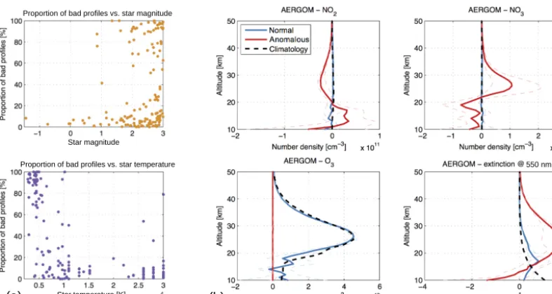
(a) (b) Star magnitude

Star temperature [K]

Proportion of bad profiles vs. star temperature Proportion of bad profiles vs. star magnitude

550 nm

Figure 1. (a) Proportion of anomalous profiles as a function of star temperature and magnitude.(b) Median gas and aerosol extinction

profiles for normal and anomalous AerGOM retrievals calculated using 200 profiles.

polynomial inλ−1with 350, 550 and 750 nm set as reference wavelengths.

For more details on the AerGOM retrieval algorithm, we refer the interested reader to Sect. 3 of the companion paper (Vanhellemont et al., 2016).

2.3 Anomalous profiles and stellar occultation parameters

During the development phase of AerGOM, it was discov-ered that while the algorithm had beneficial properties re-garding the retrieval of stratospheric aerosol profiles, it did have a drawback compared to the operational algorithm, namely that some of the converging retrievals exhibited some non-physical behaviour leading to incorrect retrievals of O3, NO2, NO3and aerosol extinction profiles. These so-called “anomalous profiles” were mostly retrieved for occul-tations carried out with either a dim (Mstar>2) and/or a cold (Tstar<5×103K) star, as shown in Fig. 1a. A comparison of gaseous and aerosol profiles between normal AerGOM re-trievals and anomalous profiles is shown in Fig. 1b. The data, calculated from the median of 200 profiles, show that anoma-lous profiles have no ozone, which is compensated above 20 km by negative NO2 profiles, very large values of NO3 and enhanced aerosol extinction.

The reason for the retrieval of such profiles by AerGOM was due to a combination of low signal-to-noise ratio (SNR) of the transmittance at shorter wavelengths for dim and cold stars, and an inadequate a priori of gaseous and aerosol species. The operational retrieval sidestepped this issue by using first a DOAS method to retrieve NO2 and NO3, re-moving their contribution from the measured signal before carrying out ozone and aerosol retrieval.

This problem has now been fixed by using full clima-tologies of gas and aerosol species as a priori for the spec-tral inversion. However, this finding prompted the consider-ation that some of the retrievals might be affected by occul-tation parameters such as star properties and solar zenith an-gle (SZA) that could lead to stray light, and occultation obliq-uity which is an important factor in the imperfect correction of atmospheric scintillation (Sofieva et al., 2009). Therefore, another aspect of this intercomparison involves studying the consistency of the agreement of AerGOM aerosol retrievals with those of other instruments under various occultation conditions. Section 6 presents the results of these compar-isons.

3 Intercomparison instruments

(5)

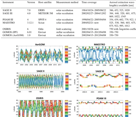
Table 1.Characteristics of the stratospheric aerosol extinction datasets used in this work.

Instrument Version Host satellite Measurement method Time coverage Aerosol extinction

wave-length(s) available [nm]

SAGE II 7.0 ERBS solar occultation 1984/10/24–2005/08/22 386, 452, 525, 1020

SAGE III 4.0 METEOR 3M solar occultation 2002/02/27–2004/12/02 384, 448, 520, 601, 675, 755,

869, 1022, 1545

POAM III 4 SPOT-4 solar occultation 1998/04/22–2005/04/04 354, 439, 602, 779, 922, 1020

MAESTRO 3.12.1 Scisat solar occultation 2004/02/21–now 525, 530, 560, 603, 675, 779,

875, 922, 995, 1012

OSIRIS 6 Odin limb scattering 2001/10/28–now 750 with Ångström coefficient

GOMOS (IPF) 6.01 Envisat stellar occultation 2002/04/15–2012/04/08 350–750

GOMOS (AerGOM) 1.0 Envisat stellar occultation 2002/04/15–2012/04/08 350–750

AerGOM

SAGE III

POAM III SAGE II

MAESTRO

OSIRIS

Figure 2.Latitude and temporal coverage for the various instruments used for the intercomparisons. The number of observations per month

is calculated for a 10◦latitude bin. The colour code gives the number of observations per month.

In this paper, we opted for the approach of comparing mea-surements with multiple instruments’ datasets. The power of this approach is that by uncovering similar and/or consistent features across the many available measurements, some sort of consensus can be reached on the agreement of the data. The weakness of such methodology is that there is no clear independent source of high-quality information, and consen-sus does not imply any form of absolute truth.

For this work, the SAGE II, SAGE III, POAM III, MAE-STRO and OSIRIS instruments are used as a basis for the in-tercomparison efforts with AerGOM. Table 1 provides some general information about these instruments and their respec-tive stratospheric aerosol products.

Figure 2 shows the spatio-temporal coverage of the datasets used for this study. Note that the colour scale

indi-cating zonally averaged observations per month in a 10◦

lat-itude bin is different for each experiment. There is a vast dif-ference (a factor of 3–4) in coverage from a limb instrument (OSIRIS) compared with solar occultation experiments. GO-MOS coverage is more extensive than what is shown in Fig. 2 for AerGOM, but to ensure high-quality data, all observa-tions that could potentially be stray-light-contaminated were filtered out resulting in a limited coverage at high latitudes.

3.1 SAGE II

(6)

during a mission that lasted from October 1984 until August 2005. The instrument recorded the attenuation of sunlight by the Earth’s atmosphere in seven spectral channels between 386 and 1020 nm during each sunrise and sunset encoun-tered by the spacecraft. The measurements were separated into slant path optical depth contributions for O3, NO2, H2O and aerosol at four channels (386, 452, 525 and 1020 nm) using a least-squares technique (Thomason et al., 2008).

In this work, we use the SAGE II v7.0 stratospheric aerosol dataset (Damadeo et al., 2013) for which the 386 nm aerosol channel is not recommended due to some unexplained con-tribution that can be substantial (approaching 30 %) at low extinction levels. Therefore, this channel is not considered in the comparisons. Note also that the aerosol extinction co-efficient measurements at 452 nm do not reliably extend be-low 12 km and will not be used bebe-low this altitude, whereas measurements made at 525 nm are reliable in the UTLS and available as low as 5 km despite substantial impacts by ozone absorption and molecular scattering (Thomason and Vernier, 2013).

3.2 SAGE III

SAGE III was launched in December 2001 on-board the Rus-sian METEOR 3M spacecraft. It gathered data from Febru-ary 2002 until the end of the mission in March 2006, using the technique of solar occultation. It observed the line-of-sight (LOS) transmission profiles from 0.5 to 100 km at 87 wavelengths from the ultraviolet to the near-infrared with an estimated 0.7 km vertical resolution.

Aerosol extinction is derived in nine spectral channels by removing the effects of molecular scattering, O3and NO2 ab-sorption. The precision and accuracy of the aerosol product is linked to the measurement noise in the channel, the qual-ity of the Global Modeling and Assimilation Office (GMAO) density product, the noise and bias in the retrieved O3and NO2, and the consistency of the cross sections used in the O3/NO2 multi-linear regression retrieval and those at the aerosol channel wavelengths.

It was found that the aerosol extinction coefficient mea-surements at 448, 520, 755, 869, and 1021 nm are reliable with accuracies and precisions on the order of 10 % in the 15–25 km range (Thomason et al., 2010). It is recommended to only exploit the 385 nm measurements above 16 km where the accuracy is on a par with other aerosol channels. Aerosol measurements at 601 and 676 nm will not be used in the present study because of the large measurement noise of the channel and poor accuracy of the retrieved extinction, respec-tively.

3.3 POAM III

The Polar Ozone and Aerosol Measurement Instrument (POAM III) (Lumpe et al., 2002; Randall et al., 2001) was

launched in March 1998 on the Satellite Pour l’Observation de la Terre (SPOT 4) in a sun-synchronous polar orbit.

The instrument used the solar occultation technique to measure atmospheric transmission across nine spectral chan-nels in the UV–Vis range. From these measurements, O3, NO2, H2O and O2vertical profiles can be retrieved. Strato-spheric aerosols are also retrieved at several wavelengths (354, 439, 602, 778, 922, 1020 nm) up to an altitude of ap-proximately 25 km.

POAM III sunrise aerosol extinction measurements at both 1020 and 450 nm are within±30 % of SAGE II. However, POAM III exhibits a significant sunrise–sunset bias in its extinction measurements that leads to poorer agreement be-tween SAGE II and the POAM III sunset data. This is im-portant for this work since collocations with GOMOS ob-servations are only found for POAM III sunset occultations. POAM III sunset aerosol extinctions at 1020 nm and 440 nm both exhibit a positive bias with respect to SAGE II, whose magnitude changes with altitude but can be as large as 50 %. 3.4 MAESTRO

The Atmospheric Chemistry Experiment (ACE) mission (Bernath et al., 2005) was launched on 12 August 2003 on-board the SCISAT satellite and is still currently operational. The satellite is in a low-Earth circular orbit at an altitude of 650 km and 74◦ inclination. The ACE mission is com-prised of two instruments: a Fourier transform spectrome-ter (ACE-FTS) and the Measurement of Aerosol Extinction in the Stratosphere and Troposphere Retrieved by Occulta-tion instrument (MAESTRO) (McElroy et al., 2007, 2013). The MAESTRO instrument uses the solar occultation tech-nique and is made of two independent spectrophotometers, one measuring in the UV (285–550 nm, 1.5 nm spectral res-olution) while the other observes in the VIS–NIR spectral region (525–1020 nm, 2 nm spectral resolution). These mea-surements allow the retrieval of atmospheric species such as O3, NO2, H2O, O2and aerosols. Measurements are made at tangent altitudes between 0 and 150 km (using measurements between 100 and 150 km to determine the sun reference spec-trum) and allow for a best-case vertical resolution of 1.2 km at a tangent height of 22 km. The aerosol extinction is re-trieved at 525, 530, 560, 603, 675, 779, 875, 922, 995 and 1012 nm wavelengths. Cirrus clouds are not filtered from the dataset.

(7)

3.5 OSIRIS

The Optical Spectrograph and InfraRed Imaging System (Llewellyn et al., 2004), on-board Odin, measures the ver-tical distribution of atmospheric limb radiance spectra. The satellite was launched in February 2001 in a sun-synchronous polar orbit and continues full operation at the time of writing. The local time of the ascending node is 18:00 LT, providing measurements of the sunlit summer hemisphere, global mea-surements during equinox, and a limited coverage of the win-ter hemisphere.

The two sub-systems of OSIRIS are an optical spectro-graph (OS) and an infrared imager (IRI). The optical spec-trograph consists essentially of a grating and a CCD detector, and measures the limb radiance spectra from 280 to 800 nm with a spectral resolution of approximately 1 nm (Bourassa et al., 2007). The sampling resolution of the measurements is approximately 2 km.

The IRI is composed of three vertical near-infrared chan-nels that capture one-dimensional images of the limb radi-ance at 1.26, 1.27, and 1.53 µm at a tangent altitude reso-lution of approximately 1 km. OSIRIS aerosol data product version 5 is derived using only the optical spectrograph mea-surements, and an alternate dataset (version 6) exploits both instruments for the retrieval of the aerosol extinction profiles (Rieger et al., 2014), allowing a better characterization of the aerosol scattering phase function and improving the retrieval substantially. The drawback of this new approach is that re-trievals are noisier and have a tendency to saturate at low altitudes and high aerosol loadings such as in the centre of volcanic plumes. It is this latest version (v6) of the OSIRIS dataset that is used in this study. However, the comparison results presented in this paper can be generalized to OSIRIS aerosol extinction v5 dataset at 750 nm, as there are very little differences between both datasets when it comes to AerGOM comparisons.

It is important to note that the OSIRIS dataset v6 is based on measured radiances at 750 and 1530 nm, from which an Ångström exponent is derived. In this work, we per-form comparisons with OSIRIS extinction at 750 nm but also at wavelengths outside the range used to determine the Ångström exponent (350 and 550 nm).

4 Methodology

The comparison of datasets is based on the statistical analy-sis of collocated events, defined here as observations within a distance1r=500 km and a period±1t=12 h from each other. Since stratospheric aerosols are assumed to be slowly varying over time and space in the absence of volcanic activ-ity, these criteria are deemed acceptable. It should be noted that processes such as pyro-convective events, other tropo-spheric intrusions and polar stratotropo-spheric clouds can also sig-nificantly change the extinction signal in the stratosphere and therefore make it more difficult to compare data points that

are further apart. The key is to strike a balance between the proximity of observations in time and space and the number of sample observations available for analysis. Evaluation of different collocation criteria showed that constraining further the1t and1rgenerally does not affect the final results but sometimes lead to undersampling.

The relative difference between the AerGOM extinction

βAerGOMand the extinction from a collocated measurement

βi from dataseti(in %) is

100×

βAerGOM−βi(λ)

βi(λ)

. (4)

All observations with a relative uncertainty larger than 100 % are discarded before performing the analysis in order to avoid biasing the results due to inferior quality data, but it should be noted that using all observations does not alter the re-sults significantly. The profiles are interpolated on a com-mon 1 km spacing vertical grid using a linear interpolation method. AerGOM extinctions are interpolated at the wave-length(s) of the other instruments using Eq. (2). In this way, a distribution of values is obtained for each tangent altitude

zand wavelength λ and the final results are derived from this distribution by calculating the interquartile mean and the semi-interquartile range, which should be robust estimates of the average value and the variability, respectively.

5 Comparison of collocated profiles

Figure 3 shows the results of the intercomparison of Aer-GOM against all datasets from Table 1 using the method out-lined in Sect. 4. Three different aspects of the comparison are shown: the relative difference (interquartile mean), the rela-tive difference variability (semi-interquartile range), and the absolute aerosol extinction profiles of AerGOM and the other datasets (interquartile mean). The total number of colloca-tions is also indicated and varies widely from one dataset to the next. To quantify the effect of the change in retrieval algo-rithm from IPF to AerGOM, the comparisons were also per-formed using IPF and the results are shown as dashed lines in the relative difference and the variability plots.

5.1 AerGOM comparison with other datasets

Overall, the agreement between AerGOM and other datasets for tangent altitudes between 15 and 30 km is typically within

(8)

10−6 10−5 10−4 10−3 10−2 10 15 20 25 30 35 Extinction [km−1] Altitude [km]

*mean2575* AerGOM−IPF, good_aergom_data

(IPF) 350 nm (AerGOM) 350 nm (IPF) 550 nm (AerGOM) 550 nm (IPF) 756 nm (AerGOM) 756 nm

10−6

10−5

10−4

10−3

10−2

10 15 20 25 30 35

Extinction [km−1]

Altitude [km]

*mean2575* AerGOM−OSIRIS, good_aergom_data

10−6

10−5

10−4

10−3

10−2

10 15 20 25 30 35

Extinction [km−1]

Altitude [km]

*mean2575* AerGOM−OSIRIS, good_aergom_data (OSIRIS) 350 nm (AerGOM) 350 nm (OSIRIS) 550 nm (AerGOM) 550 nm (OSIRIS) 756 nm (AerGOM) 756 nm

10−6 10−5

10−4 10−3

10−2 10 15 20 25 30 35 Extinction [km−1] Altitude [km]

*mean2575* AerGOM−MAESTRO, good_aergom_data

10−6 10−5

10−4 10−3

10−2 10 15 20 25 30 35 Extinction [km−1] Altitude [km]

(MAESTRO) 525 nm (AerGOM) 525 nm (MAESTRO) 603 nm (AerGOM) 603 nm (MAESTRO) 675 nm (AerGOM) 675 nm (MAESTRO) 779 nm (AerGOM) 779 nm 10−6

10−5 10−4

10−3 10−2 10 15 20 25 30 35

Extinction [km−1]

Altitude [km]

*mean2575* AerGOM−POAM III, good_aergom_data

10−6 10−5

10−4 10−3

10−2 10 15 20 25 30 35

Extinction [km−1]

Altitude [km]

(POAM III) 354 nm (AerGOM) 354 nm (POAM III) 439 nm (AerGOM) 439 nm (POAM III) 602 nm (AerGOM) 602 nm (POAM III) 778 nm (AerGOM) 778 nm 10−6

10−5 10−4

10−3 10−2 10 15 20 25 30 35

Extinction [km−1]

Altitude [km]

*mean2575* AerGOM−SAGE III, good_aergom_data

10−6 10−5

10−4 10−3

10−2 10 15 20 25 30 35

Extinction [km−1]

Altitude [km]

(SAGE III) 384 nm (AerGOM) 384 nm (SAGE III) 448 nm (AerGOM) 448 nm (SAGE III) 520 nm (AerGOM) 520 nm (SAGE III) 755 nm (AerGOM) 755 nm 10−6

10−5 10−4

10−3 10−2 10 15 20 25 30 35

Extinction [km−1]

Altitude [km]

mean2575 AerGOM−SAGE II, good_aergom_data

10−6 10−5

10−4 10−3

10−2 10 15 20 25 30 35

Extinction [km−1]

Altitude [km]

*mean2575* AerGOM−SAGE II, good_aergom_data

(SAGE II) 452 nm (AerGOM) 452 nm (SAGE II) 525 nm (AerGOM) 525 nm

0 25 50 75 100 125 150 175 200

10 15 20 25 30 35 (AerGOM−IPF)/(IPF) [%] Altitude [km]

*siqr* AerGOM−IPF, good_aergom_data

0 25 50 75 100 125 150 175 200 10 15 20 25 30 35 (AerGOM−IPF)/(IPF) [%] Altitude [km]

*siqr* AerGOM−IPF, good_aergom_data

350 nm 550 nm 756 nm

−100 −75 −50 −25 0 25 50 75 100 10 15 20 25 30 35

(AerGOM−IPF)/(IPF) [%]

Altitude [km]

−100 −75 −50 −25 0 25 50 75 100 10 15 20 25 30 35

(AerGOM−IPF)/(IPF) [%]

Altitude [km]

350 nm 550 nm 756 nm

0 25 50 75 100 125 150 175 200 10 15 20 25 30 35

(AerGOM−OSIRIS)/(OSIRIS) [%]

Altitude [km]

*siqr* AerGOM−OSIRIS, good_aergom_data

0 25 50 75 100 125 150 175 200 10 15 20 25 30 35

Altitude [km]

*siqr* AerGOM−OSIRIS, good_aergom_data

350 nm 550 nm 756 nm

−100 −75 −50 −25 0 25 50 75 100

10 15 20 25 30 35 (AerGOM−OSIRIS)/(OSIRIS) [%] Altitude [km]

−100 −75 −50 −25 0 25 50 75 100

350 nm 550 nm 756 nm

0 25 50 75 100 125 150 175 200 10 15 20 25 30 35 (AerGOM−MAESTRO)/(MAESTRO) [%] Altitude [km]

*siqr* AerGOM−MAESTRO, good_aergom_data

0 25 50 75 100 125 150 175 200 10 15 20 25 30 35 (AerGOM−MAESTRO)/(MAESTRO) [%] Altitude [km]

*siqr* AerGOM−MAESTRO, good_aergom_data

525 nm 603 nm 675 nm 779 nm 0 25 50 75 100 125 150 175 200

10 15 20 25 30 35

(AerGOM−POAM III)/(POAM III) [%]

Altitude [km]

*siqr* AerGOM−POAM III, good_aergom_data

0 25 50 75 100 125 150 175 200 10 15 20 25 30 35

Altitude [km]

*siqr* AerGOM−POAM III, good_aergom_data

354 nm 439 nm 602 nm 778 nm

−100 −75 −50 −25 0 25 50 75 100 10 15 20 25 30 35

Altitude [km]

−100 −75 −50 −25 0 25 50 75 100 10 15 20 25 30 35

Altitude [km]

*mean2575* AerGOM−POAM III, good_aergom_data 354 nm 439 nm 602 nm 778 nm

0 25 50 75 100 125 150 175 200

10 15 20 25 30 35

(AerGOM−SAGE III)/(SAGE III) [%]

Altitude [km]

*siqr* AerGOM−SAGE III, good_aergom_data

0 25 50 75 100 125 150 175 200

10 15 20 25 30 35

Altitude [km]

*siqr* AerGOM−SAGE III, good_aergom_data

384 nm 448 nm 520 nm 755 nm

−100 −75 −50 −25 0 25 50 75 100 10 15 20 25 30 35

Altitude [km]

−100 −75 −50 −25 0 25 50 75 100 10 15 20 25 30 35

Altitude [km]

384 nm 448 nm 520 nm 755 nm

0 25 50 75 100 125 150 175 200

10 15 20 25 30 35

(AerGOM−SAGE II)/(SAGE II) [%]

Altitude [km]

siqr AerGOM−SAGE II, good_aergom_data

0 25 50 75 100 125 150 175 200

10 15 20 25 30 35

Altitude [km]

*siqr* AerGOM−SAGE II, good_aergom_data

452 nm 525 nm

MAESTRO SAGE II

−200 −150−100 −50 0 50 100 150 200 10 15 20 25 30 35 (aergom−sage3)/(sage3) [%] Altitude [km] aergom−sage3 comparison

−200 −150 −100 −50 0 50 100 150 200 10 15 20 25 30 35 (aergom−sage3)/(sage3) [%] Altitude [km] aergom−sage3 comparison 384 nm 448 nm 520 nm 755 nm Relative difference (Interquartile mean) Absolute extinction (Interquartile mean) OSIRIS IPF 6.01 N=1017 N=1364 N=13625 N=20000 Relative difference variability

(Semi-interquartile range)

0 50 100 150 200 250 300 10 15 20 25 30 35

(aergom−gopr)/(gopr) [%]

Altitude [km]

*siqr* aergom−gopr, good_aergom_data

0 50 100 150 200 250 300 10 15 20 25 30 35

(aergom−gopr)/(gopr) [%]

Altitude [km]

*siqr* aergom−gopr, good_aergom_data

350 nm 550 nm 756 nm (aergom-maestro)/(maestro) [%] SAGE III N=3158 POAM III N=634 750

−100 −75 −50 −25 0 25 50 75 100 10 15 20 25 30 35

Altitude [km]

−100 −75 −50 −25 0 25 50 75 100 10 15 20 25 30 35

Altitude [km]

mean2575 AerGOM−SAGE II, good_aergom_data

452 nm 525 nm

−100 −75 −50 −25 0 25 50 75 100 10 15 20 25 30 35

(AerGOM−MAESTRO)/(MAESTRO) [%]

Altitude [km]

−100 −75 −50 −25 0 25 50 75 100 10 15 20 25 30 35

Altitude [km]

525 nm 603 nm 675 nm 779 nm

10−6 ₁₀−5 ₁₀−4 ₁₀−3 ₁₀−2

10 15 20 25 30 35

Extinction [km−1]

Altitude [km]

10−6 ₁₀−5 ₁₀−4 ₁₀−3 ₁₀−2

10 15 20 25 30 35

Extinction [km−1]

Altitude [km]

*mean2575* AerGOM−SAGE II, good_aergom_data (SAGE II) 452 nm (AerGOM) 452 nm (SAGE II) 525 nm (AerGOM) 525 nm

(SAGE III) 384 nm (AerGOM) 384 nm (SAGE III) 448 nm (AerGOM) 448 nm (SAGE III) 520 nm (AerGOM) 520 nm (SAGE III) 755 nm (AerGOM) 755 nm

10−6 ₁₀−5 ₁₀−4 ₁₀−3 ₁₀−2

10 15 20 25 30 35 Extinction [km−1] Altitude [km]

10−6 ₁₀−5 ₁₀−4 ₁₀−3 ₁₀−2

10 15 20 25 30 35 Extinction [km−1] Altitude [km]

(POAM III) 354 nm (AerGOM) 354 nm (POAM III) 439 nm (AerGOM) 439 nm (POAM III) 602 nm (AerGOM) 602 nm (POAM III) 778 nm (AerGOM) 778 nm

10−6

10−5

10−4

10−3

10−2

10 15 20 25 30 35

Extinction [km−1]

Altitude [km]

10−6

10−5

10−4

10−3

10−2

10 15 20 25 30 35

Extinction [km−1]

Altitude [km]

(MAESTRO) 525 nm (AerGOM) 525 nm (MAESTRO) 603 nm (AerGOM) 603 nm (MAESTRO) 675 nm (AerGOM) 675 nm (MAESTRO) 779 nm (AerGOM) 779 nm

10−6 10−5 10−4 10−3 10−2 10 15 20 25 30 35

Extinction [km−1]

Altitude [km]

10−6 10−5 10−4 10−3 10−2 10 15 20 25 30 35

Extinction [km−1]

Altitude [km]

*mean2575* AerGOM−OSIRIS, good_aergom_data (OSIRIS) 350 nm (AerGOM) 350 nm (OSIRIS) 550 nm (AerGOM) 550 nm (OSIRIS) 756 nm (AerGOM) 756 nm

750 750

10−6 ₁₀−5 ₁₀−4 ₁₀−3 ₁₀−2

10 15 20 25 30 35

Extinction [km−1]

Altitude [km]

10−6 ₁₀−5 ₁₀−4 ₁₀−3 ₁₀−2

10 15 20 25 30 35

Extinction [km−1]

Altitude [km]

(IPF) 350 nm (AerGOM) 350 nm (IPF) 550 nm (AerGOM) 550 nm (IPF) 756 nm (AerGOM) 756 nm

Figure 3. Relative difference (left panels), variability of the relative difference (central panels) and absolute aerosol extinction vertical

profiles (right panels) for each dataset (SAGE II, SAGE III, POAM III, MAESTRO, OSIRIS and IPF) at various wavelengths compared with collocated AerGOM profiles. The dashed curves in the relative difference plots were calculated using IPF v6.01 instead of AerGOM. The

(9)

25 km), indicating potential issues with the data. It is also sur-prising that the 520 nm extinction is the most biased within this altitude and spectral range, as one would expect it to be most accurate for AerGOM.

According to the work of Damadeo et al. (2013), the 525 nm aerosol extinction measurements from SAGE II ver-sion 7.0 and SAGE III verver-sion 4.0 should agree to within a few percent. It is therefore puzzling to see such differences in the intercomparisons of AerGOM with both instruments. The reason for the discrepancy is that the SAGE II and SAGE III data are not sampled in the same way when it comes to AerGOM collocations, with SAGE III data found solely in the southern hemispheric mid-latitudes, whereas collocations with SAGE II measurements are found at all latitudes. Re-sults from Sect. 6.3 show that the bias varies based on the latitude of observation, and when comparing results from the same latitude bands, the intercomparisons are consistent with the results from Damadeo et al. (2013). For POAM III com-parisons below 700 nm and above 20 km, biases are similar to what is seen in SAGE III but shifted by 15 %.

Below 20 km, comparisons between AerGOM extinction at shorter (λ <700 nm) wavelengths and SAGE II, SAGE III and POAM III extinctions show a strong positive bias, in-creasing with dein-creasing altitude. This positive bias is larger for shorter wavelengths. These features could be the result of subvisible cirrus clouds present in the field of view, but it is unclear why only these datasets are affected while compar-isons with MAESTRO and OSIRIS show no such large pos-itive biases, and why the effect is much more pronounced in the case of AerGOM than for comparisons with IPF. The lat-ter result suggests that the AerGOM retrieval algorithm itself must be the cause of this bias, not the GOMOS instrument, despite its known decreasing SNR with decreasing tangent altitude. Section 6.3 takes a closer look at the potential effect of clouds on the results from the perspective of latitude of observation.

The results of the comparison between AerGOM and MAESTRO extinction profiles at shorter (λ <700 nm) wave-lengths show a different behaviour of the relative difference than seen in the other comparisons. AerGOM is negatively biased compared with MAESTRO, with values of the bi-ases ranging from −35 to −50 %. The bias is quite con-stant within an altitude range of 10 to 25 km. Above 25 km, all AerGOM extinctions become increasingly negatively bi-ased with regards to MAESTRO with increasing altitude and wavelength. These results seem to confirm the issues sus-pected with the MAESTRO dataset, namely that it retrieves too large aerosol extinctions. Based on the AerGOM compar-ison, this effect increases with the wavelength of observation. One surprising feature of the comparison is the small vari-ability (25 %) of the relative difference with AerGOM, al-most constant between 10 and 25 km and for all wavelengths. OSIRIS data at wavelengths below 750 nm are extrapo-lated and should be used cautiously, but it is nevertheless interesting to see that there is a pretty good agreement

be-tween AerGOM and OSIRIS at 550 nm, with an almost con-stant negative bias of 25 % between 15 and 30 km. For shorter wavelengths however, the comparison shows that OSIRIS ex-tinctions are much larger than AerGOM above 20 km.

Looking at comparisons of AerGOM aerosol extinction profiles forλ >700 nm, one can see that there is clearly a problem with AerGOM results at larger wavelengths, de-spite the use of GOMOS transmission data from spectrom-eter B1 that should have improved the aerosol retrieval in this spectral region. There is a strong negative bias above 25–30 km with respect to all other datasets (especially clear with SAGE III, MAESTRO and OSIRIS) that increases to-wards higher altitudes. Above 27 km, retrieved extinctions atλ >700 nm are mostly negative, hence the large negative biases observed. These large discrepancies could very well be due to the use of outdated ozone cross sections. It was mentioned in Thomason et al. (2010) that anomalous aerosol extinctions in the SAGE III 755 nm channel from previous versions of the dataset were caused by the use of an out-dated ozone cross section that had errors of the order of 10 % in the Chappuis band. Preliminary work to improve the trace gas cross sections used with AerGOM seems to con-firm that such changes can lead to a significant improvement of the aerosol extinction values for λ >700 nm, especially above 25 km. Looking at the AerGOM absolute extinction profiles atλ >700 nm, one notices that there are more ver-tical structures than for the other wavelengths, with a small peak around 16 km, and troughs near 13 and 20 km. Interest-ingly, these structures are also seen in the comparison results with IPF at all wavelengths and, hence, seem to be some-what linked to the measurement method or to some aspect of the retrieval that is common to both AerGOM and IPF algo-rithms.

The variability of the extinction comparisons in the 350– 600 nm spectral range increases with decreasing tangent al-titudes and is larger for shorter wavelengths. This is ex-pected, as it simply follows the spatial and spectral behaviour of the GOMOS SNR, and is confirmed by the similar IPF comparison variability. The dispersion of the comparisons at

λ >700 nm is less systematic but tends to increase dramati-cally with tangent altitudes above 20–25 km, correlated with the strong negative bias.

For reference purposes, we also show the comparison be-tween AerGOM and IPF profiles in the bottom panel of Fig. 3. The results are based on 20 000 randomly chosen GO-MOS observations spanning different geolocations and oc-cultation parameters. Even though the raw data come from the same instrument, the comparison shows substantial dif-ferences.

5.2 Differences between AerGOM and IPF

(10)

4710 C. É. Robert et al.: Intercomparisons of AerGOM stratospheric extinctions

101 102 103 104

10 15 20 25 30 35

Altitude [km]

*std* AerGOM−SAGE III, good_aergom_data

101 102 103 104

10 15 20 25 30 35

Altitude [km]

384 nm 448 nm 520 nm 755 nm

101 ₁₀2 ₁₀3 ₁₀4

10 15 20 25 30 35

Altitude [km]

101 ₁₀2 ₁₀3 ₁₀4

10 15 20 25 30 35

Altitude [km]

384 nm 448 nm 520 nm 755 nm

750

0

2000

4000

6000

10

15

20

25

30

35

Number of data points available

Altitude [km]

aergom

−

osiris,

λ

=350nm

0

2000

4000

6000

8000

10

15

20

25

30

35

Number of data points available

Altitude [km]

aergom

−

osiris,

λ

=550nm

0

2000

4000

6000

10

15

20

25

30

35

Altitude [km]

aergom

−

osiris,

λ

=756nm

[

−

90

−

60]

[

−

60

−

30]

[

−

30 0]

[0 30]

[30 60]

0

2000

4000

6000

10

15

20

25

30

35

Altitude [km]

0

2000

4000

6000

8000

10

15

20

25

30

35

Altitude [km]

0

2000

4000

6000

10

15

20

25

30

35

Altitude [km]

[

−

90

−

60]

[

−

60

−

30]

[

−

30 0]

[0 30]

[30 60]

lat -90, -60

0

100

200

300

400

500

5

10

15

20

25

30

35

40

Altitude [km]

lat

−

90,

−

90

lat

−

60,

−

60

lat

−

30,

−

30

lat 0, 0

lat 30, 30

lat -60, -30

lat -30, 0

lat 0, 30

lat 30, 60

0

2000

4000

6000

10

15

20

25

30

35

Altitude [km]

aergom

−

osiris,

λ

=350nm

0

2000

4000

6000

8000

10

15

20

25

30

35

Altitude [km]

aergom

−

osiris,

λ

=550nm

0

2000

4000

6000

10

15

20

25

30

35

Altitude [km]

aergom

−

osiris,

λ

=756nm

[

−

90

−

60]

[

−

60

−

30]

[

−

30 0]

[0 30]

[30 60]

lat -90, -60

lat -60, -30

lat -30, 0

lat

0, 30

lat 30, 60

101 102 103 104 10 15 20 25 30 35

Altitude [km]

*std* AerGOM−SAGE II, good_aergom_data

101 102 103 104 10 15 20 25 30 35

Altitude [km]

452 nm 525 nm 101 102 103 104 10 15 20 25 30 35

Altitude [km]

*std* AerGOM−OSIRIS, good_aergom_data

101 102 103 104 10 15 20 25 30 35

Altitude [km]

350 nm 550 nm 756 nm

101 102 103 104

10 15 20 25 30 35

Altitude [km]

101 102 103 104

10 15 20 25 30 35

Altitude [km]

350 nm 550 nm 756 nm 750

SAGE II SAGE III OSIRIS

Figure 4.Standard deviation of the aerosol extinction relative difference for AerGOM (solid) and IPF (dashed) comparisons with SAGE II,

SAGE III and OSIRIS. Note that the abscissa is scaled logarithmically.

IPF. In several cases (SAGE II, SAGE III and POAM III) and more specifically for observations below 20 km and for

λ <700 nm, the IPF results are in better agreement with the correlative measurements than AerGOM, giving rise to the question of whether AerGOM can be considered an improve-ment over IPF.

Vanhellemont et al. (2016) show that the conceptual im-provements of AerGOM are translated into aerosol extinction profiles that are better behaved than those of IPF v6.01, with AerGOM results being particularly less noisy than their IPF counterparts and having a more realistic spectral dependence. However, since the present work averages a large number of profiles to obtain the results and does so in a robust way by using the interquartile mean and the semi-interquartile range as a metric of the central tendency and dispersion, respec-tively, the noise in the IPF data is no longer a concern. There-fore under certain conditions, despite the fact that the IPF v6.01 aerosol dataset is noisier and hence less precise, it is more accurate than AerGOM.

One of the great strengths of AerGOM however is its higher precision, which is quantified in the variability. It can already be seen from Fig. 3 that the variability of AerGOM comparison results is typically smaller than those made with IPF, especially between 15 and 30 km. Then again, these re-sults are only based on 50 % of the data. If instead of the semi-interquartile range, one uses the standard deviation as a measure of the variability, consequently using the entire dis-tribution of data, the real advantage of AerGOM over IPF becomes clear. Figure 4 shows the standard deviation of the relative difference on a logarithmic scale for comparisons of AerGOM (solid) and IPF (dashed) with SAGE II, SAGE III and OSIRIS as a function of altitude. Not only is the dis-persion of IPF results larger than those of AerGOM below 30 km, it is not uncommon for it to be more than an order of magnitude larger. The variability of the IPF comparisons becomes larger as the wavelength considered is far from 500 nm, the reference wavelength for the spectral model used in IPF.

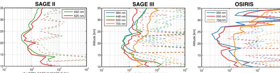
Of course, one would hope that a dataset is both precise and accurate, and it is meaningful to search for ways to improve the current AerGOM dataset so that it agrees bet-ter with SAGE II and SAGE III, both considered excellent aerosol extinction datasets. There are several ways in which the AerGOM algorithm settings can be modified to improve its retrieval of stratospheric aerosols such as using improved trace gas absorption cross sections or using a full covariance matrix when performing the inversion. But one particular as-pect of AerGOM seems to have a large effect on the aerosol extinction in the UTLS, namely the aerosol spectral law cho-sen to model the aerosol extinction cross section. The cur-rent version of AerGOM uses a second-degree polynomial inλ−1, but some preliminary results show that using a poly-nomial of degree 1 instead significantly improves the results below 20 km. These results are shown in Fig. 5, where a mod-ified AerGOM algorithm using a polynomial of degree 1 in

λ−1as spectral law was used to generate a new dataset that was then compared with SAGE II and SAGE III. The im-provements below 20 km are clear, with biases being limited to within 25 % above 12 km for SAGE II, and within±50 % for SAGE III. While more work is needed, this seems to show that slight modifications to the algorithm settings can lead to results that are more in line with those of the SAGE instru-ments.

6 Bias variability with star and occultation parameters Section 5 described AerGOM’s bias relative to other instru-ments, but it did not take into account the very specific fea-tures of GOMOS which do not concern the other sensors but may dramatically affect the quality of AerGOM extinction. Specifically, the use of a wide range of stellar sources with very different characteristics, the subsequent low value of the SNR, and the versatility of the occultation configuration re-flected in the obliquity and the solar zenith angle may all affect the GOMOS measurements.

(11)

Aer-C. É. Robert et al.: Intercomparisons of AerGOM stratospheric extinctions 4711

−100 −75 −50 −25 0 25 50 75 100

10 15 20 25 30 35

Altitude [km]

−100 −75 −50 −25 0 25 50 75 100

10 15 20 25 30 35

Altitude [km]

384 nm 448 nm 520 nm 755 nm

101 102 103 104

10 15 20 25 30 35

Altitude [km]

101 102 103 104

10 15 20 25 30 35

Altitude [km]

384 nm 448 nm 520 nm 755 nm 101 102 103 104 10 15 20 25 30 35

Altitude [km]

101 102 103 104 10 15 20 25 30 35

Altitude [km]

384 nm 448 nm 520 nm 755 nm

750

0

2000

4000

6000

10

15

20

25

30

35

Number of data points available

Altitude [km]

aergom

−

osiris,

λ

=350nm

0

2000

4000

6000

8000

10

15

20

25

30

35

Altitude [km]

aergom

−

osiris,

λ

=550nm

0

2000

4000

6000

10

15

20

25

30

35

Altitude [km]

aergom

−

osiris,

λ

=756nm

[

−

90

−

60]

[

−

60

−

30]

[

−

30 0]

[0 30]

[30 60]

0

2000

4000

6000

10

15

20

25

30

35

Altitude [km]

0

2000

4000

6000

8000

10

15

20

25

30

35

Altitude [km]

0

2000

4000

6000

10

15

20

25

30

35

Altitude [km]

[

−

90

−

60]

[

−

60

−

30]

[

−

30 0]

[0 30]

[30 60]

lat -90, -60

0

100

200

300

400

500

5

10

15

20

25

30

35

40

Altitude [km]

lat

−

90,

−

90

lat

−

60,

−

60

lat

−

30,

−

30

lat 0, 0

lat 30, 30

lat -60, -30

lat -30, 0

lat 0, 30

lat 30, 60

0

2000

4000

6000

10

15

20

25

30

35

Altitude [km]

aergom

−

osiris,

λ

=350nm

0

2000

4000

6000

8000

10

15

20

25

30

35

Altitude [km]

aergom

−

osiris,

λ

=550nm

0

2000

4000

6000

10

15

20

25

30

35

Altitude [km]

aergom

−

osiris,

λ

=756nm

[

−

90

−

60]

[

−

60

−

30]

[

−

30 0]

[0 30]

[30 60]

lat -90, -60

lat -60, -30

lat -30, 0

lat

0, 30

lat 30, 60

101 102 103 104 10 15 20 25 30 35

Altitude [km]

101 102 103 104 10 15 20 25 30 35

Altitude [km]

452 nm 525 nm

101 102 103 104

10 15 20 25 30 35

Altitude [km]

101 102 103 104

10 15 20 25 30 35

Altitude [km]

350 nm 550 nm 756 nm

101 102 103 104

350 nm 550 nm 756 nm750

SAGE II SAGE III OSIRIS

−100 −75 −50 −25 0 25 50 75 100

10 15 20 25 30 35

Altitude [km]

−100 −75 −50 −25 0 25 50 75 100

10 15 20 25 30 35

Altitude [km]

452 nm 525 nm

SAGE II SAGE III

Figure 5.Relative difference of aerosol extinction comparisons between a modified AerGOM dataset using a different spectral law

(poly-nomial of degree 1 inλ−1) and SAGE II and SAGE III datasets at different wavelengths. These results show a better agreement between

AerGOM and both SAGE instruments below 20 km.

GOM and other instruments. For each instrument, compar-isons were carried out as explained in Sect. 4, except that only a specific subset of collocated profiles corresponding to particular criteria was used to calculate the interquartile mean. The parameters under investigation are star properties, solar zenith angle and latitude of observation. A study of the effect of the obliquity on the bias was carried out, but the re-sults did not bear any concluding evidence of a repercussion on the AerGOM measurements and were therefore omitted from the discussion. Note that this analysis is only valid for the AerGOM retrieval and cannot be generalized to the IPF dataset. Due to the very large variability of the comparisons between POAM III and AerGOM observed in the last sec-tion, POAM III results are not included in this part of the work.

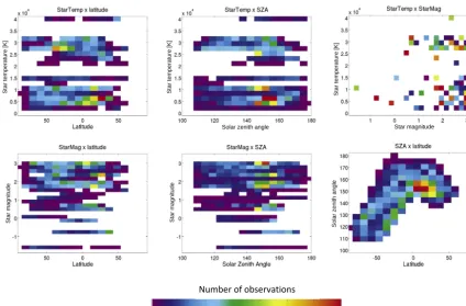
Studying the effects of a given occultation parameter or star property assumes that only one variable will change while all other parameters are constant, but this is not al-ways the case for GOMOS. Most parameters are somewhat interdependent, albeit very loosely in some cases. Figure 6 gives an overview of the interdependence of several parame-ters: star magnitude, star temperature, latitude and SZA. The figure shows 2-D histograms of the number of observations for different combinations of these occultation parameters, taking into account only dark limb GOMOS observations. From these graphs, one can see for instance that at low SZA (≤120◦), almost no bright stars are available and mostly only dim stars will be used for occultation. Maybe the clearest and most important dependence among the occultation parame-ters is observed for solar zenith angles and latitudes of obser-vations, where low SZA values correspond to high latitudes and equatorial observations to high SZA values. We must therefore be cautious when analysing the results of compar-isons with regards to certain occultation parameters and take into account this interdependence.

Table 2.Classes of star properties (as defined in this work).

Star temperatures Descriptor Star Descriptor

103K magnitudes

0–6 cold −1.5–1.5 bright

6–26 mid-cold 1.5–2.3 mid-bright

26–40 hot 2.3–3 dim

6.1 Star properties

The properties of stars (star temperatureTstarand magnitude

Mstar) used as light source by GOMOS largely determine the shape of its spectral irradiance: cold (hot) stars have larger spectral irradiance at longer (shorter) wavelengths. In addi-tion, the magnitude of the star might mitigate or aggravate the impact of the shape of the spectral irradiance on the qual-ity of the retrieval by altering further the SNR in different spectral regions. In particular, it could be expected that dim stars seriously affect results at short (long) wavelengths for cold (hot) stars. Table 2 details the nine distinct categories of stars that we have defined for this work and that we will consider, ranging from dim and cold to hot and bright.

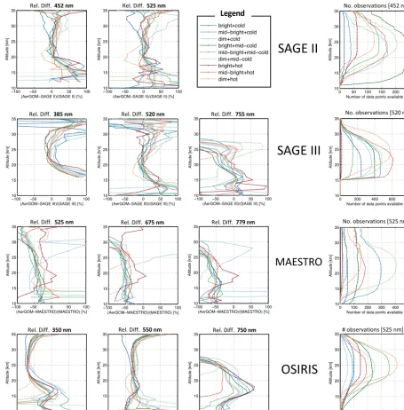
Figure 7 presents the results of the comparisons between AerGOM and the other datasets at various wavelengths and according to the defined star classes. The rightmost panel shows the number of observations available to perform the comparisons. Note that in some cases, the number of obser-vations is very limited so that the effects seen in these cases may be strongly affected by subsampling.

(12)

Number'of'observations

Star temperature [K] Star temperature [K] _{Star temperature [K]}

Star magnitude Star magnitude

Solar zenith angle

Solar zenith angle Star magnitude

Figure 6.Interdependence of the GOMOS occultation parameters depicted using 2-D histograms of the number of observations for different

combinations of occultation parameters (star temperature and magnitude, solar zenith angle and latitude of observation).

AerGOM–OSIRIS comparison at 750 nm, the bias can vary from−300 % for dim–hot stars to +50 % for bright–hot stars at 17 km.

The occultation star properties have the largest influ-ence on AerGOM extinctions when considering dim–hot stars, especially for AerGOM aerosol extinction at wave-lengths larger than 650 nm. The effect can also be seen at 550 nm but to a more limited extent. For SAGE II (452, 525 nm), SAGE III (520 nm), MAESTRO (525 nm) and OSIRIS (550 nm), AerGOM is more negatively biased be-tween approximately 15 and 20 km.

At shorter wavelengths (<400 nm), the AerGOM com-parison for cold star occultations also shows a different be-haviour with respect to the other star property comparisons, but the effect is much less dramatic and not consistent across the various datasets. For SAGE III, dim–cold star occulta-tions are very negatively biased between 17 and 23 km with regards to the other occultations but are positively biased be-tween 25 and 35 km. Overall, in this short wavelength range, the weakness of the signal from dim–cold stars is responsi-ble for the erratic behaviour of the bias profile at the lowest altitudes toward the troposphere.

6.2 Solar zenith angle

Another parameter studied is the solar zenith angle at which the stellar occultation was carried out. SZA is an indicator of

the local time, although there is no reason to believe that this can affect the extinction comparisons. Here, we assume that the dependence of the AerGOM results on the SZA, if any, is due to stray light as there is a larger probability that stray light finds its way into the instrument as the SZA decreases.

The AerGOM aerosol retrieval is only carried out for ob-servations made in partially or completely dark limb, mean-ing that the SZA of observations will vary between 100 and 180◦. There is already a stray-light correction applied to GO-MOS Level 1 product, but an evaluation of the AerGOM dataset seems to show some residual stray-light contamina-tion in the data.

(13)

−100 −50 0 50 100 10 15 20 25 30 35 (AerGOM−OSIRIS)/(OSIRIS) [%] Altitude [km]

*mean2575* , λ=350nm

−100 −50 0 50 100

*mean2575* , λ=550nm

−100 −50 0 50 100

*mean2575* , λ=756nm

−100 −50 0 50 100

10 15 20 25 30 35

Altitude [km]

*mean2575* , λ=525nm

−100 −50 0 50 100

10 15 20 25 30 35

Altitude [km]

*mean2575* , λ=603nm

−100 −50 0 10 15 20 25 30 35 (AerGOM− Altitude [km] *mean2575* ,

−100 −50 0 50 100

10 15 20 25 30 35

Altitude [km]

*mean2575* , λ=779nm

−100 −50 0 50 100

10 15 20 25 30 35 (AerGOM−MAESTRO)/(MAESTRO) [%] Altitude [km]

*mean2575* , λ=603nm

−100 −50 0 50 100

*mean2575* , λ=675nm

−100 −50 0 50 100

*mean2575* , λ=525nm

−100 −50 0 50 100

*mean2575* , λ=603nm

−100 −50 0 50 100

*mean2575* , λ=675nm

−100 −50 0 50 100

*mean2575* , λ=779nm

−100 −50 0 50 100

10 15 20 25 30 35

Altitude [km]

*mean2575* , λ=384.2687nm

−100 −50 0 50 100

10 15 20 25 30 35

Altitude [km]

*mean2575* , λ=448.5182nm

−100 −50 0

10 15 20 25 30 35 (AerGOM− Altitude [km]

*mean2575* , λ

−100 −50 0 50 100

10 15 20 25 30 35

Altitude [km]

*mean2575* , λ=755.3782nm

−100 −50 0 50 100

10 15 20 25 30 35

Altitude [km]

*mean2575* , λ=448.5182nm

−100 −50 0 50 100

10 15 20 25 30 35

Altitude [km]

*mean2575* , λ=520.312nm

−100 −50 0 50 100

10 15 20 25 30 35

Altitude [km]

*mean2575* , λ=384.2687nm

−100 −50 0 50 100

10 15 20 25 30 35

Altitude [km]

*mean2575* , λ=448.5182nm

−100 −50 0 50 100

10 15 20 25 30 35

Altitude [km]

*mean2575* , λ=520.312nm

−100 −50 0 50 100

10 15 20 25 30 35

Altitude [km]

*mean2575* , λ=755.3782nm

−100 −50 0 50 100

10 15 20 25 30 35

Altitude [km]

*mean2575* , λ=452nm

−100 −50 0 50 100

10 15 20 25 30 35

Altitude [km]

*mean2575* , λ=525nm

0 1000 2000 3000 4000 5000 10 15 20 25 30 35

Altitude [km]

aergom−osiris, λ=350nm

0 1000 2000 3000 4000 5000 10 15 20 25 30 35

Altitude [km]

aergom−osiris, λ=550nm

0 100 200 300 400 500

10 15 20 25 30 35

Altitude [km]

aergom−ace, λ=525nm

0 100 200 300

10 15 20 25 30 35

Altitude [km] aergom−ace, λ=779nm bright+cold mid−bright+cold dim+cold bright+mid−cold mid−bright+mid−cold dim+mid−cold bright+hot mid−bright+hot dim+hot

0 200 400 600 800 10 15 20 25 30 35

Altitude [km]

aergom−sage3, λ=384.2687nm

0 200 400 600 800 10 15 20 25 30 35

Altitude [km]

0 200 400 600 800 10 15 20 25 30 35

Altitude [km]

0 200 400 600 10 15 20 25 30 35

Altitude [km]

aergom−sage3, λ=755.3782nm bright+cold mid−bright+cold dim+cold bright+mid−cold mid−bright+mid−cold dim+mid−cold bright+hot mid−bright+hot dim+hot

0 50 100 150 200 250

10 15 20 25 30 35

Altitude [km]

aergom−sage2, λ=452nm

Rel.0Diff.00452$nm Rel.0Diff.00525$nm No.0observations0[4520nm]

No.0observations0[5200nm]

Rel.0Diff.00385$nm Rel.0Diff.00520$nm Rel.0Diff.00755$nm

SAGE0III

No.0observations0[5250nm]

SAGE0II

MAESTRO

#0observations0[5250nm]

OSIRIS

Legend

0 100 200 300

10 15 20 25 30 35

Altitude [km]

AerGOM−MAESTRO, λ=779nm bright+cold mid−bright+cold dim+cold bright+mid−cold mid−bright+mid−cold dim+mid−cold bright+hot mid−bright+hot dim+hot

Figure 7.Relative differences between AerGOM and SAGE II, SAGE III, MAESTRO and OSIRIS datasets for different star categories,

ranging from dim–cold to bright–hot (left panels). The rightmost panel presents the number of observations for each dataset comparison and star category.

These results strongly suggest the presence of stray light, as it should increase the number of photons detected by the spectrometer, hence artificially increasing the value of the transmission and decreasing the retrieved extinction. If this decrease in extinction is attributed to the aerosol (which has a slow varying spectral dependence unlike ozone, NO2and NO3), then the comparison should show a decrease of the positive bias. If we assume the stray light to be more or less constant with altitude, its relative effect should be larger at high altitudes (>25 km) and longer wavelengths, due to the

generally much smaller aerosol extinction values typically found for such cases.

6.3 Latitude

(14)

−100 −50 0 50 100 10 15 20 25 30 35

Altitude [km]

*mean2575* , λ=350nm

−100 −50 0 50 100 10 15 20 25 30 35

Altitude [km]

*mean2575* , λ=550nm

−100 −50 0 50 100 10 15 20 25 30 35

Altitude [km]

*mean2575* , λ=756nm

−100 −50 0 50 100

*mean2575* , λ=525nm

<

AerGOM, an improved algorithm for stratospheric aerosol extinction retrieval from GOMOS observations – Part 2: Intercomparisons