www.nonlin-processes-geophys.net/15/943/2008/ © Author(s) 2008. This work is distributed under the Creative Commons Attribution 3.0 License.
Nonlinear Processes
in Geophysics
Patch behaviour and predictability properties of modelled
finite-amplitude sand ridges on the inner shelf
N. C. Vis-Star1, H. E. de Swart1, and D. Calvete2
1Institute for Marine and Atmospheric research, Utrecht University, Princetonplein 5, 3584 CC Utrecht, The Netherlands 2Dept. de F´ısica Aplicada, Universitat Polit`ecnica de Catalunya, Campus Nord, Jordi Girona, 08034 Barcelona, Spain
Received: 3 September 2008 – Revised: 4 November 2008 – Accepted: 4 November 2008 – Published: 8 December 2008
Abstract. The long-term evolution of shoreface-connected sand ridges is investigated with a nonlinear spectral model which governs the dynamics of waves, currents, sediment transport and the bed level on the inner shelf. Wave vari-ables are calculated with a shoaling-refraction model instead of using a parameterisation. The spectral model describes the time evolution of amplitudes of known eigenmodes of the linearised system. Bottom pattern formation occurs if the transverse bottom slope of the inner shelf, β, exceeds a critical valueβc. For fixed model parameters the sensi-tivity of the properties of modelled sand ridges to changes in the number(N−1)of resolved subharmonics (of the ini-tially fastest growing mode) is investigated. For anyN the model shows the growth and subsequent saturation of the height of the sand ridges. The saturation time scale is sev-eral thousands of years, which suggests that observed sand ridges have not reached their saturated stage yet. The migra-tion speed of the ridges and the average longshore spacing between successive crests in the saturated state differ from those in the initial state. Analysis of the potential energy bal-ance of the ridges reveals that bed slope-induced sediment transport is crucial for the saturation process. In the tran-sient stage the shoreface-connected ridges occur in patches. The overall characteristics of the bedforms (saturation time, final maximum height, average longshore spacing, migra-tion speed) hardly vary withN. However, individual time series of modal amplitudes and bottom patterns strongly de-pend onN, thereby implying that the detailed evolution of sand ridges can only be predicted over a limited time inter-val. Additional experiments show that the critical bed slope βc increases with larger offshore angles of wave incidence,
Correspondence to: H. E. de Swart
larger offshore wave heights and longer wave periods, and that the corresponding maximum height of the ridges de-creases whilst the saturation time inde-creases.
1 Introduction
Field data collected at various storm-dominated inner shelves of coastal seas (depths of 5−20 m) reveal the presence of patches of large-scale shoreface-connected sand ridges (Du-ane et al., 1972; Swift and Field, 1981; Dyer and Huntley, 1999; Harrison et al., 2003, and references herein), hereafter abbreviated as sfcr. Typically, a patch consists of 4−8 sfcr, where the latter have heights of several meters and are spaced several kilometers apart. The ridges make an angle of 20-50◦with the storm-driven current along the coast, such that
their seaward ends are shifted upstream with respect to their attachments to the shoreface. Furthermore, the ridges have asymmetrical profiles, with gentle slopes on the landward (upstream) sides and steep slopes on the seaward (down-stream) sides. The estimated evolution time of sfcr is several thousands of years and they migrate several meters per year in the downstream direction. As these ridges seem to affect the stability of the beach (Van de Meene and Van Rijn, 2000), gaining more understanding about their behaviour is relevant for coastal zone management purposes.
Θ
s
H
rms,s V
2π/κ
outer shelf inner shelf
shoreface
x=0
Ls
H0
Hs
z
x
z=0
y
Fig. 1. Schematic representation of a typical time-averaged bottom
topography of the continental shelf, representing the inner and outer shelf. Forcing of the water motion is due to (obliquely) incident waves and a storm-driven current. Symbols are explained in the text.
sediment by the waves. Improvements with respect to the Trowbridge model were i) the occurrence of a preferred mode, ii) the results are hardly sensitive to the cross-shore profile of the storm-driven current and iii) the predicted spac-ing between successive ridges, as well as their growth rate and migration speed are in fair agreement with field data if all these effects are accounted for.
Calvete and De Swart (2003) investigated the long-term dynamics of sfcr by expanding the flow and bottom pertur-bations in a truncated series of eigenmodes. The result is a set of equations describing the time evolution of the ampli-tudes. They showed that after the initial growth stage ridge profiles become asymmetric and reach a finite height. They also found that adding subharmonic modes (eigenmodes with wavelengths being larger than that of the most preferred mode) causes the spacing between successive ridges in the saturated state to be larger than that during the initial stage.
The models cited above have two important drawbacks. First, stirring of sediment by waves is described by a severe parameterisation. Second, they do not provide an explanation for the patchiness of observed sfcr. Therefore, in this paper a new nonlinear model will be presented, in which processes like shoaling and refraction are explicitly accounted for. This was also done in recent studies by Lane and Restrepo (2007) and Vis-Star et al. (2007), but they only examined the initial formation of sfcr. Here, an analysis will be presented of the long-term behaviour of sfcr in dependence of offshore wave characteristics and the transverse bottom slope of the inner shelf. Specific emphasis is put on the role of subharmonics in generating patches of sfcr. This is because adding subhar-monics implies a higher resolution in the spectral domain,
thereby potentially allowing for the occurrence of group (or modulation) behaviour. The physical processes controlling the migration and saturation behaviour will be identified by analysing the energy balance of the bedforms. Our method extends the one used by Garnier et al. (2006) in the sense that also the instantaneous global longshore migration speed is investigated.
The model is presented in Sect. 2, after which the method of analysis is discussed in Sect. 3. In Sect. 4 the results are presented, followed by a discussion in Sect. 5 and the con-clusions in Sect. 6.
2 Model
We adopt the model formulation of Vis-Star et al. (2007). The coupled dynamics of waves, storm-driven currents and the sandy bed is considered on an idealised inner shelf (see Fig. 1). The latter is bounded on the landward side x=0 by the transition to the shoreface (depthH0) and at the
sea-ward side (x=Ls) by the outer shelf (depthHs). The mean transverse bottom slope isβ=(Hs−H0) /Ls. The water mo-tion is forced by imposed wave condimo-tions at the outer shelf (offshore angle of wave incidence2s, offshore root-mean-square wave heightHrms,s and wave period T) and a wind stress that forces a net current. Sand is only transported dur-ing severe weather conditions (which occur±5% of the time) and is the result of the joint action of waves (stirring sand from the bottom) and a longshore storm-driven flow (caus-ing net sand transport). Hence, the model is representative for storms. After application of the rigid-lid approximation (sea surface elevationmean depth) and the quasi-steady approach (hydrodynamics adjusts instantaneously to a new bed level), the wave equations are
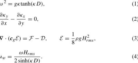
ω2=gκtanh(κD), (1)
∂κy ∂x −
∂κx
∂y =0, (2)
∇·(cgE)=F−D, E=
1 8ρgH
2
rms, (3)
uw = ωHrms
2 sinh(κD). (4)
energy dissipation by bottom friction. In the definition for the wave energy densityρ is the water density andHrms is the square wave height. Finally, the root-mean-square amplitude of the near-bed wave orbital motion uw (hereafter called wave orbital velocity) depends on the other variables and is input in the modules for the current and the sediment transport.
The currents are described by the quasi-steady depth-averaged shallow water equations
(v·∇)v+fez×v= −g∇zs+
τs−τb
ρD , (5)
∇·(Dv)=0, (6)
τs =τsyey, τb=ρruwv. (7)
Here,vdenotes the depth- and wave-averaged flow velocity with componentsuandv in thex- andy-direction, respec-tively, andz=zs is the level of the mean sea surface. Further-more, f is the Coriolis parameter, ez is the unity vector in thez-direction,τsis the wind stress vector,τbthe mean bed shear-stress vector andey is a unit vector in the longshore direction. Note thatτbdepends linearly on the current (fric-tion coefficientr), as waves are strong compared to currents during stormy weather.
The bed evolution equation and the formulations for the sediment transport read
(1−p)∂zb
∂t +∇·qb+∇·qs =0, (8)
qb=
3 2νbu
2
w(v−λbuw∇zb)=qb,a+qb,d, (9)
qs =Cv−λsu5w∇zb=qs,a+qs,d, (10)
∇·(Cv)=αu3w−γ C
D. (11)
In Eqs. (8)–(11)tis time,pis the porosity of the bed,z=zb is the bed level, andqbandqsdenote the wave-averaged sed-iment transport as bedload and suspended load, respectively. The latter two are divided into advective partsq.,aand diffu-sive partsq.,d (related to bed slopes). In the expressions for bedload and suspended load transportνb,αandγare known coefficients,Cis the depth-integrated volumetric concentra-tion of sediment andλbandλs are the bed slope parameters for bedload and suspended load, respectively.
Note that the expressions forqb,a andqs,a in Eqs. (9)– (10) do not contain any net advective transport due to waves. This is a consequence of the assumption that, although wave orbital motion is strong compared to currents, the wave pro-files are symmetric. Moreover, it is assumed thatuwis much larger than the critical velocityuc for erosion of sediment, so the influence ofucon sediment transport is not explicitly modelled.
As boundary conditions offshore wave properties (root-mean-square wave height, period and angle of wave inci-dence) are imposed. Furthermore, the cross-shore flow com-ponentuvanishes atx=0 and far offshore, the bed levelzb is kept fixed at these two positions and the sediment concen-tration vanishes far from the coast.
3 Method of analysis
3.1 Basic state and linear stability analysis
From here on primary wave variables are denoted by X=(κ, θ,E) and other dependent variables by 9=(u, v, zs,C, zb). The system of equations of mo-tion of Sect. 2 allows for a basic state that is steady and longshore uniform. It is characterised by a shelf topography z=−H (x), an incoming wave field with wavenumberK(x), angle of wave incidence 2(x) and wave energy E(x), a storm-driven currentv=(U (x), V (x)), a free surface eleva-tion ξ(x) and a depth-integrated volumetric concentration of sediment C(x). Hence, X=Xb(x)=(K, 2, E) and 9=9b(x)=(U, V , ξ, C,−H ). BothXband9bare defined in Vis-Star et al. (2007); in particular U (x)=0 and V (x) results from a balance between the longshore wind stress and bottom stress. The basic state describes shoaling and refracting waves and a storm-driven flow along the coast.
The stability properties of the basic state are considered by studying the dynamics of small perturbations evolving on this basic state. Hence,
9 =9b+90, (12)
and90(x, y, t )=(u0, v0, η0, c0, h0)denote the perturbed vari-ables, which are assumed to have small values with respect to their basic state values. In principle, also perturbations in the wave variables have to be considered:X=Xb+X0. Sim-ilar as in previous studies, we assumeX0=0. Physically, this
means that wave-topography interactions, i.e., wave refrac-tion and shoaling and dissiparefrac-tion of wave energy due to the presence of bedforms are neglected. We will return to this aspect in Sect. 5.
Substitution of Eq. (12) into the equations of motion of Sect. 2 and linearizing the results yields the system
S∂9
0
∂t =L9
0
. (13)
The 5×5 matrixS contains the temporal information of the perturbations and has one non-zero element:S(5,5)=1−p. The linear matrix operatorL contains all the linear terms; its elements are given in Appendix A. This system admits solutions
in an eigenvalue problem, whereσ are the eigenvalues and ˜
ψ (x) the eigenfunctions. This problem can be solved by standard methods. The eigenmode that has the largest growth rateσr≡<e(σ )is called the initially most preferred mode; it has a wavenumberk=kp, with a corresponding wavelength `p=2π/ kp, and a migration speedVm=−=m(σ )/ kp. 3.1.1 Nonlinear analysis
In order to investigate the long-term evolution of sfcr the full set of nonlinear equations
S∂9
0
∂t =L9
0+N(90) (15)
for the perturbations has to be considered. Here,S andL
are as in the linearised system Eq. (13), whilstN(90)is the nonlinear vector operator, which includes all nonlinear terms in the equations of motion for the perturbations. The ex-pression for the nonlinear vector operatorN is also given in Appendix A.
Following Calvete and De Swart (2003) the perturbations are written as
90(x, y, t )=90(x, t )+ψ (x, y, t ), (16)
where the unknown contributions90have a longshore
uni-form structure and the contributionsψ are expanded into a truncated series of (known) eigenmodes of the linear system:
ψ= <e
J
X
j=1
Nj
X
nj=1 ˇ
ψj nj(t )ψ˜j nj(x)exp(ikjy)
. (17)
For each alongshore wavenumberkj,nj refers to the cross-shore modenumber,ψˇj nj(t )are the unknown modal ampli-tudes andψ˜j nj(x)the known cross-shore structures of the eigenfunctions of the linear problem. Furthermore, J and Nj are the largest longshore and cross-shore mode number, respectively. Expansions Eqs. (16) and (17) are substituted in the nonlinear equations of motion. After averaging over the alongshore direction, equations are obtained for the long-shore uniform flow modes and bottom mode, which are sub-sequently subtracted from the original equations. The results are projected onto the adjoint linear eigenmodes. This pro-cedure yields a set of nonlinear algebraic equations for the flow amplitudesuj nˇ j,vj nˇ j,ηj nˇ j andcj nˇ j and a set of non-linear differential equations for the amplitudes of the bottom modeshj nˇ j. A third-order time integration scheme is used to solve the resulting system of equations (see Karniadakis et al., 1991).
Here, the choice is to include the most preferred mode with wavenumberkp(largest initial growth rate) in the non-linear expansion, as we are interested whether it is still the dominant mode in the bottom pattern on the long term. Fur-thermore, several superharmonics and generally some sub-harmonics are used, such that a total numberJ of different
longshore wavenumbers kj is included. Thus, if only su-perharmonics are included, the system is solved on a domain with longshore lengthLy=2π/ kp. By including (N−1) sub-harmonic modes the domain becomes longer:Ly=2π N/ kp. In both cases periodic boundary conditions in the longshore direction are applied. Modes that fit into the domain have wavenumberskj=2πj/Ly=Njkp (j=1,2,3, . . .). An indi-vidual mode is denoted by (j/N, nj).
3.1.2 Energy balance of the bedforms
In order to investigate the saturation behaviour of bedforms Garnier et al. (2006) developed a method to study the global properties of the bedforms on the whole domain. It boils down to deriving a potential energy balance of bottom per-turbations by multiplying the linearised version of the bed evolution Eq. (8) with the bed elevationh0 and integrating over the whole domain. It reads
(1−p) ∂ ∂t
1 2|h|
2=P +1, (18)
where
|h| =(h02)12, (19)
P = qb,a+qs,a·∇h0, (20) 1= − νbλbu3
w+λsu5w
|∇h0|2. (21)
Note that12|h|2measures the potential energy density of the bedforms and the overbar indicates the average over the do-main. Equation (21) results from application of Green’s the-orem and the definitions forqb,d andqs,d. TermP, which describes the production of potential energy due to the advec-tive bedload and suspended load transport, is posiadvec-tive if the advective sediment transport and bed slopes are positively correlated. Term 1 describes the loss of potential energy due to bedslope-induced sediment transport.
An instantaneous global growth rate of the sfcrσr˜ is de-fined as
˜ σr ≡
1 |h|2
∂
∂t
1
2|h|
2
. (22)
The definition is such that if the bed pattern is represented by a single waveh0=<enh(x)e˜ iky+σ to, thenσr˜ →σr, i.e., the initial growth rate. A new variable that is considered in this study is the instantaneous global longshore migration speed, defined as
˜ Vm= −
1
∂h0 ∂y
2
∂h0
∂y ∂h0
∂t . (23)
4 Results
4.1 Parameter setting
Runs were performed with parameter values that are rep-resentative for the micro-tidal inner shelf of Long Island, located at latitude∼40◦ N. Here, a patch of 8 sfcr is ob-served (Duane et al., 1972). The depth varies fromH0=14 m
to Hs=20 m over an inner shelf width of Ls=5.5 km (β=1.1×10⁻³). However, the default experiment is per-formed for an inner shelf slope which is approximately 25% of its observed value. The motivation for the latter choice is that the behaviour of the system for larger values of β is not principally different, but a much higher number of eigenmodes is required to obtain accurate solutions. This aspect will be further discussed in Sect. 5. The alongshore wind stressτsy=−0.4 N m−2, the offshore root-mean-square wave height Hrms,s=1.5 m, the wave period T=11 s and the offshore angle of wave incidence2s=−20◦(waves ap-proach from the northeast). Values of the other parame-ters are: r=2.0×10⁻³, νb=5.6×10⁻⁵ s2 m−1, λb=0.65, λs=7.5×10⁻⁴s4m−3,α/γ=9.5×10−5s3m−3andp=0.4. A motivation for these choices can be found in Vis-Star et al. (2007). Results of the simulations are shown for continuous storm conditions.
In the default caseN=10. In the time integration a time step of about 1 full-storm year was used. Both adding more modes and decreasing the time step did not change the solu-tions.
4.2 Linear stability analysis and eigenmodes
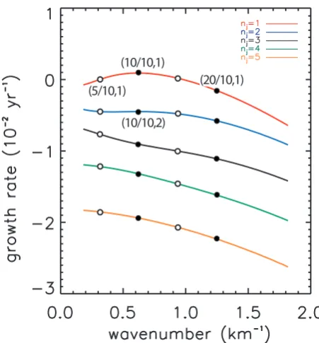
Figure 2 shows the initial growth rate σr as a function of the longshore wavenumberk for the default parameter set-ting. The largest growth rate is attained fork=kp∼0.6 km−1. Thus, the initially most preferred mode has a longshore wavelengthλp∼10 km, ane-folding time scaleTg∼1100 yr and a migration speed Vm∼−26 m yr−1. If N=10 this mode is labeled (10/10,1). Its bottom pattern, as well as that of the (5/10,1) subharmonic mode, the (20/10,1) superhar-monic mode and the (10/10,2) secondary cross-shore mode is shown in Fig. 3. Further details about the results of the linear stability analysis are shown in Supplementary Note 1 (see http://www.nonlin-processes-geophys.net/15/943/2008/ npg-15-943-2008-supplement.zip).
4.3 Patch behaviour and sensitivity to number of subhar-monics
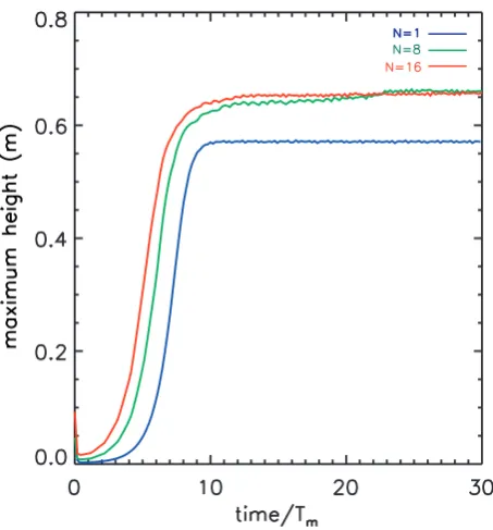
The temporal evolution of the maximum height of the bed-forms is shown in Fig. 4 for differentN. At t=0 all re-solved bottom modes have small amplitudes (in the order of 0.1 mm) and random phases. At first, scale selection takes place: all resolved modes initially have the same amplitude and it takes time before the fastest growing mode dominates over the other modes. Next, a stage occurs in which the
(10/10,1)
(20/10,1)
(10/10,2) (5/10,1)
Fig. 2. Linear growth rates for cross-shore modenjas a function of
the longshore wavenumber. The most preferred mode is indicated
by (10/10,1). The solid dots indicate modes that are included in
the nonlinear analysis forN=1. The open dots represent additional
modes included ifN=2.
height of the bedforms grows exponentially, followed by sat-uration towards a constant finite value. The satsat-uration time scale is defined as the time at which the maximum height is 98% of its value in the saturated state. IfN=1 (no subhar-monics) saturation of the bedform height takes place after a period of∼9000 yr at a value of 0.57 m. If subharmonics are included the final height is larger (∼0.66 m) and the satura-tion time is slightly longer. However, both the increase in the finite bedform height and saturation time are almost indepen-dent of the choice of numberN. It turns out that the satura-tion time also hardly depends on the initial amplitude of the resolved modes. This is because for larger initial amplitudes the stage of scale selection becomes longer, whilst the stage of exponential growth becomes almost equally shorter.
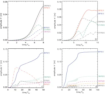
The time evolution of the amplitude of the individual modes resolved yields information about their mutual inter-actions. Figure 5 shows forN=10 the time evolution of the five largest bottom modes att /Tm∼8, t /Tm∼15,t /Tm∼50 andt /Tm∼100. For the present bottom slope (β=2.7×10⁻⁴) the morphodynamic time scaleTm∼1000 yr.
mode (5/10,1) mode (10/10,1) mode (20/10,1)
a) b) c)
V V V V
mode (10/10,2)
d)
Fig. 3. Bottom pattern (light: crests, dark: troughs) for (a) subharmonic mode (5/10,1), (b) preferred mode (10/10,1), (c) superharmonic mode (20/10,1) and (d) mode (10/10,2). The arrow indicates the direction of the basic state longshore velocity.
Fig. 4. Maximum height of the bedforms versust /Tmfor model
runs in which (N−1) subharmonic modes are included. For the
present bottom slopeTm∼1000 yr, whereas for the realistic slope
Tm∼100 yr.
dominant than the initially most preferred mode. Note that, although the bedform height is saturated fort /Tm&8, the am-plitudes of the individual modes are not and thus the length scale and shape of the bedforms are still changing. Slightly aftert /Tm=15, the (9/10,1) mode rapidly decreases in am-plitude, whereas the (8/10,1) mode increases in amplitude and becomes dominant. Just before t /Tm∼50 the initially most preferred mode disappears from the graph and is no longer one of the five largest bottom modes. It takes a very long time before the amplitudes of the individual modes are more or less saturated. The wavelength of the saturated bed-forms is dominated by the (8/10,1) mode and is approxi-mately 108×10=12.5 km. Furthermore, a difference in the height of individual bars and depths of individual troughs can be observed. The lengthening of patterns is consistent with Calvete and De Swart (2003) and Garnier et al. (2006), although the shift in length scale is smaller than in these stud-ies.
a) b)
c) d)
(9/10,1)
(8/10,1)
(10/10,1)
(11/10,1)
(17/10,1)
(8/10,1)
(16/10,1)
(16/10,2)
(24/10,2)
(24/10,1) (10/10,1)
(9/10,1)
(8/10,1) (11/10,1) (19/10,1)
(8/10,1)
(16/10,1)
(7/10,1)
(16/10,2) (9/10,1)
Fig. 5. Time evolution of the amplitude of the five bottom modes which have the largest amplitude at (a)t /Tm∼8, (b)t /Tm∼15, (c)
t /Tm∼50 and (d)t /Tm∼100. For the present bottom slopeTm∼1000 yr, whereas for the realistic slopeTm∼100 yr. Modes are indicated by
a specific colour and denoted as (j/N,nj), wherejis the longshore modenumber, (N−1) the amount of subharmonic modes included andnj
the cross-shore modenumber, respectively. Line style (solid, dotted, dashed, dot-dashed, dot-dot-dashed) indicates the order of dominance of modes at the final time step. Here,N=10.
˜
˜
a)
b)
Fig. 6. Time evolution of instantaneous global (a) growth rateσ˜r and (b) migration speedV˜m. Shaded areas indicate time periods during
y
x
=
Fig. 7. Bottom pattern (light: crests, dark: troughs) att /Tm∼8 forN=8 (top),N=10 (middle) andN=16 (bottom). For the present bottom
slopeTm∼1000 yr, whereas for the realistic slopeTm∼100 yr. The shoreface is at the top and left is downstream. Here, the longshore extent
of the domain is∼N `p.
y (km) x (km)
t/Tm=1
t/Tm=5
t/T m=8
t/T m=20
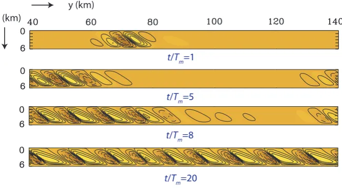
Fig. 8. Bottom pattern (light: crests, dark: troughs) at different timest /Tm;N=10. For the present bottom slopeTm∼1000 yr, whereas for
the realistic slopeTm∼100 yr. The shoreface is at the top and left is downstream. Here, the longshore extent of the domain is∼N `p.
system it turns out that the group velocity of its linear eigen-modes is larger than the phase velocity.
The time evolution of the amplitude of the five fastest growing modes depends strongly on the amount of subhar-monics included in the calculations. In case ofN=8,N=12 orN=16, a period oft /Tm∼60 is not sufficient to reach sat-uration of the amplitudes of individual modes, whereas for N=10 modal amplitudes are saturated after that period. This sensitivity to N is remarkable, as Fig. 4 indicates that the saturation time scale for the bedform height shows only a very weak dependence onN. IfN=8, modal amplitudes be-come constant aftert∼100Tm. At that time the (7/8,1) mode is dominates over all others, which indicates a wavelength of the final bedforms of approximately 87×10=11.4 km. If N=12 saturation of amplitudes occurs only aftert /Tm∼200 and at that time the (10/12,1) mode is dominant, indicat-ing a wavelength of the sfcr of approximately 12.0 km. If N=16, mode saturation is found after t /Tm∼300, the (13/16,1) mode is dominant and hence the wavelength of the final bedforms is∼12.3 km. These results indicate that
the wavelength of sfcr in the saturated state is in the range of 11.5−12.5 km, which denotes a mild lengthening compared to results obtained with the linear analysis.
NO GROWTH NO GROWTH
MODEL INV
ALID
MODEL INV
ALID
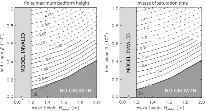
finite maximum bedform height inverse of saturation time
a) b)
Fig. 9. Contour plot of equal (a) finite maximum height (m) of the bedforms and (b) inverse of time needed for saturation (10−3yr−1) in theHrms,s−βplane. Obtained with nonlinear model (solid lines) or extrapolated (dotted lines).
time. Figure 8 shows the bottom patterns at different times for the case thatN=10. Patch behaviour of ridges is only observed during the evolution of the system towards the sat-urated state. Clearly, at timet /Tm=20 the entire domain is covered by sfcr.
Whether sfcr occur in patches or not is strongly related to the interactions between different modes in the nonlin-ear analysis. Modulation behaviour will occur when (1) the spectrum of growing modes is sufficiently narrow, and (2) the dominant modes that control the evolution of the sys-tem have comparable wavelengths and amplitudes. In the ex-periments performed with subharmonic modes the first con-dition is met, whilst the second concon-dition is only obeyed during the transient stage of the evolution. For example, Fig. 5 shows that att /Tm∼8 the (10/10,1) mode and (9/10,1) mode have comparable amplitudes. However, at a later stage (e.g.t /Tm∼20), the amplitudes of modes with successive modenumbers are not that close. In fact, obtained patterns are a superposition of the dominant mode and its superhar-monics and these imply ridge activity everywhere on the in-ner shelf.
4.4 Sensitivity results to wave characteristics
A series of runs were performed with the model without sub-harmonics (N=1) for different values of the transverse slope β (by changing the depth of the outer shelf Hs) and off-shore wave parameters 2s, Hrms,s and T. Wave parame-ters were varied one after another and other parameparame-ters kept their default values. All runs revealed that a critical trans-verse bottom slopeβchas to be exceeded before sfcr start to develop, whereβc depends on the model parameter values. Onceβ>βc the time evolution of the maximum height of the bedforms is generally characterised by growth, reduction
in growth and saturation. Numerical stable solutions could be obtained up to approximately 60% of the observed value of the slope of the inner shelf in case of no subharmonics. For larger values of β solutions become singular at some point during the evolution. Instability behaviour is related to a rapid growth of the smallest length scale included in the nonlinear analysis.
Contour plots of the finite maximum bedform height and inverse of saturation time in the2s−β plane were already presented and discussed in Vis-Star et al. (2008). It turns out that if waves approach the coast more obliquely, thenβc increases, the final height of the ridges decreases and the sat-uration time increases.
Figure 9 shows the finite maximum bedform height and in-verse of saturation time in the (Hrms,s−β) parameter space. An increase inβc from 1.0×10⁻⁴ to 4.3×10⁻⁴is obtained for an increase in the offshore root-mean-square wave height from 1.2 m to 2.0 m. Onceβ>βc, sfcr grow faster and be-come higher for smaller offshore wave heights. The depen-dence of the final height and the saturation time on the off-shore wave height is quite strong.
b)
c) d)
a)
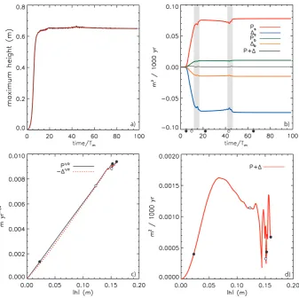
Fig. 10. (a) Time evolution of the bedforms. (b) Time evolution of production and dissipation terms due to suspended load and bedload
sediment transport and their sum. Shaded areas indicate time periods during which jumps occur in all the curves. The alternative closed en open circles below the time axis are positioned att /Tm∼5,t /Tm∼10,t /Tm∼22,t /Tm∼43 andt /Tm∼65 (aftert /Tm∼65 no change occurs).
These times are also indicated in panels c and d. For the present bottom slopeTm∼1000 yr, whereas for the realistic slopeTm∼100 yr.
(c) Square root of the production and dissipation terms as a function of|h|. (d) The sum (P+1) as a function of|h|. Here,N=10 and β=2.7×10⁻⁴.
5 Discussion
5.1 Analysis of saturation behaviour
All runs discussed in the previous section show that, starting from an initial state without bedforms, sfcr develop as free in-stabilities of the coupled water-bottom system. Their initial growth is exponentially and can be described and understood using linear stability analysis (cf. Calvete et al., 2001a). On the long term saturation behaviour occurs and the ridges at-tain a finite, almost constant height. To further understand the behaviour of the bedforms their potential energy balance is analysed. Results are shown in Fig. 10. In panel b of this figure time series are shown of the gain and loss of po-tential energy due to bedload and suspended load transport, respectively. The time periods during which jumps occur are marked. These jumps represent significant changes in com-petitive behaviour of individual bottom modes included in
the analysis, as is clear from Fig. 5. In Fig. 10c the jumps are also visible in the curves around|h|=0.15 m. Note that the time that the system needs to pass through the part of the curve for relative small bar amplitude is short compared to the time needed to approach the end of the curve. The alter-native open and closed circles below the time axis in Fig. 10b represent five specific time values which are also plotted in Fig. 10c, d. Around saturation time the increase in |h| is rather gradual. From Fig. 10d it seems that a balance be-tween production and dissipation is not reached. This, how-ever, is due to numerical accuracy, as the absolute error in the computation of both the production and dissipation term is about 3×10⁻⁷m2yr−1.
in-stantaneous global migration speed, alongshore spacing and finite amplitude, are a robust model result, independent of the amount of subharmonic modes included. However, changes in the competition between individual modes are quite un-predictable and also strongly dependent on the amount of subharmonic modes. As the bottom evolution is strongly de-pendent on parameterNthe evolution of the sfcr can only be predicted for a finite amount of time. In this context it is rel-evant to remark that Huntley et al. (2008) demonstrated that the predictability of bottom bedforms is also strongly influ-enced by the presence of defects in the initial pattern.
The lengthening of patterns in the course of time is con-sistent with that found in other nonlinear morphodynamic models, e.g., that of Coco et al. (2004) for beach cusps, that of Murray and Thieler (2004) for sorted bedforms, thay of Ashton and Murray (2006) for shoreline sand waves and the model of Garnier et al. (2006) for nearshore sand bars. The shift in length scale is similar as in Coco et al. (2004), but in the other studies the lengthening is larger.
5.2 Model limitations
In reality storms only occur during a certain time fraction (about 5%) and numbers would be a factor 20 smaller. On the other hand, taking a realistic value ofβwould cause these numbers to be larger by approximately the same factor.
In case of using a measured value of the transverse bed slope solutions become unbounded before the saturated state is reached. The results presented in this paper were obtained with a version of the model in which interactions between waves and growing bedforms were ignored. Nonlinear ex-periments including wave-topography interactions revealed spurious modes in the linear analysis which have to be fil-tered. When incorporated in the nonlinear model sfcr con-tinue to grow on the long term and numerical instabilities arise before the saturated state is reached. An explanation for the latter is that stirring of sediment by waves increases with increasing ridge height. This tendency will be coun-teracted by e.g. wave breaking, a process which is not yet implemented in the model.
The spectral method itself is also subject to limitations. The nonlinear analysis uses the solutions of the linear sys-tem as expansion modes. However, the latter are dependent on the specific parameter values used. Simulations in which strong, mild and weak storms alternate, as will be the case in reality, are feasible, but require different eigenmodes for the different realizations. This implies that several transfor-mations between the spectral domain and the physical space have to be performed, which will cause a considerable loss of accuracy.
Note that the present model assumes a constant mean sea level, whereas in several studies (cf. Swift and Field, 1981; McBride and Moslow, 1991) it is argued that sea level changes during the Holocene play an important role in the evolution of sfcr. To assess the sensitivity of model results to
H
0
Hs
Ls
A
B C H
0
+ ∆s
+
∆ Ls
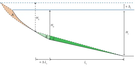
Fig. 11. Sketch of evolution of the shelf geometry under sea level
rise1s. In the case of Bruun (1954):A=B. In case of Masetti et al.
(2008):A=B+C. Other variables are defined in the text.
different sea level stands runs were performed using differ-ent cross-shore bottom profiles. The latter were constructed by generalizing the “Bruun rule” (Bruun, 1954, 1962), fol-lowing concepts discussed in Masetti et al. (2008). Start-ing from a given profile, a sea level rise1s will cause the new depth of the outer shelf to become Hs+1s (Fig. 11). Second, the depth at the transition from shoreface to inner shelf remains unchanged (valueH0), but its location shifts
landward (distance1Ls). Third, the depth profile between coastline and the inner shelf maintains its equilibrium shape and it is shifted upward and landward. The distance1Ls is calculated by imposing that the total volume of sand per unit width between coast and outer shelf remains unchanged. This results in a new transverse bottom slopeβ of the inner shelf (larger for positive1s). Experiments for different val-ues of1s were performed, starting from the default situation with subharmonics (N=10). It was found that the overall be-haviour of the model does not change if1s is varied. The main quantitative changes are that the height of the ridges in-creases (from 0.65 m to 2.2 m if1s=+1 m) and the saturation time scale decreases. This is mainly caused by the increase ofβ.
The reconstruction method we applied is highly idealised, but nevertheless yields a first idea of how sfcr might re-spond to changes in mean sea level. The numerical model of Masetti et al. (2008) is more advanced: it calculates the ex-plicit time dependence of bottom profiles under the influence of sea level rise and also accounts for the underlying stratig-raphy. Furthermore, the “Bruun rule” often yields results that do not comply with observations, because it ignores three-dimensional and site-specific aspects (Cooper and Pilkey, 2004). Ultimately, profile reconstructions should be tested against data. Such information however is not available for Long Island shelf.
5.3 Comparison with field observations
and field data is therefore limited. Generally, observations show patches of 4−8 sfcr (see literature cited in the intro-duction). In the present study we were able to reproduce the patchiness of sfcr, which was never done before. The number of sfcr per patch are consistent with the field data. The spatial patterns of the finite-amplitude sfcr exhibit typi-cal asymmetric profiles with steep slopes at the downstream sides. Extrapolating default model results to the realistic in-ner shelf bottom slope yields bedforms with a finite height of ∼4 m and a saturation time scale of∼700 yr. These values have the correct order of magnitude if compared with field data (e.g. Duane et al., 1972).
6 Conclusions
The long-term evolution of shoreface-connected sand ridges (sfcr) has been investigated and the dependence of model re-sults with respect to offshore wave properties and the inner shelf bed slope has been explored. For any forcing condi-tions (wind, waves) a critical transverse bed slope has to be exceeded before sfcr start to grow. Once this critical bed slope is exceeded, sfcr initially form as free morphodynamic instabilities and, after a stage of scale selection, their height increases exponentially in time. On the long term the sfcr attain a finite height which becomes constant and their spa-tial pattern becomes asymmetrical (mild stoss sides, steep lee sides). An analysis of the potential energy balance of the sfcr has been performed which shows that bed slope-induced sediment transport is crucial for the saturation process.
If subharmonic modes are included, sfcr also show satura-tion and the finite height increases with about 15% compared to simulations without subharmonics. The initially most pre-ferred mode is no longer dominant in the saturated state. Due to nonlinear interactions subharmonic modes dominate and cause a 20% increase in the distance between successive sfcr in time. Furthermore, the saturation time of the amplitudes of individual modes is much longer than the time scale on which the ridge height saturates. Considering the age of the sfcr, time scales of order 10Tmare realistic, which suggests that observed sfcr have not reached their final stage of devel-opment yet. In the transient stage the sfcr occur in patches and the number of ridges per patch is in the observed range of 4−8. Results indicate that the detailed evolution of the sfcr is only predictable over a finite time interval, whereas the overall characteristics (e.g. instantaneous global growth rate, instantaneous global migration speed, finite bedform height and alongshore spacing) are also predictable for long time scales. Model results are consistent with field observations.
Appendix A
Expressions for operatorsS,L,N
The symbolic form of the system of nonlinear partial differ-ential equations describing the evolution of the flow, mass, sediment concentration and bottom is given in Eq. (15), whilst Eq. (13) contains its linearised version.
Here, the elements of 5×5 matrix S (containing all the temporal information of the perturbations) are all zero, ex-cept forS(5,5)=1−p. The linear operatorLinvolves spatial derivatives and has the matrix form
L=
V∂y∂+rUw
H −f g
∂
∂x 0 0 dV
dx+f V ∂ ∂y+
rUw
H g
∂
∂y 0 0 dH
dx+H ∂
∂x H
∂
∂y 0 0 −V
∂ ∂y dC
dx+C ∂
∂x C
∂
∂y 0 V ∂ ∂y+ γ H γ C H2
L51 −3
2νbU
2
w ∂ ∂y−C
∂
∂y 0 −V ∂ ∂y L55 .(A1)
The elementsL51andL55of operatorLare
L51 = −
3 2νbU
2
w ∂
∂x−3νbUw dUw
dx − dC dx −C
∂ ∂x,
L55 =
3
2νbλb 3U
2
w dUw
dx ∂ ∂x +U
3
w ∂2 ∂x2 +U
3
w ∂2 ∂y2
!
+λs Uw5 ∂2 ∂x2+5U
4
w dUw
dx ∂ ∂x+U
5 w ∂2 ∂y2 ! .
Finally, the vectorN governs all nonlinear contributions. Its elements are
N1=u0
∂u0 ∂x +v
0∂u 0
∂y + rUwu0 H−h0 −
rUwu0 H ,
N2=u0
∂v0 ∂x +v
0∂v 0
∂y +
rUw(V+v0) H−h0 −
rUwV H−h0 −
rUwv0 H ,
N3= −u0
∂h0 ∂x −h
0∂u 0
∂x −v
0∂h 0
∂y −h
0∂v 0
∂y,
N4=c0
∂u0 ∂x +u
0∂c 0
∂x +c
0∂v 0
∂y +v
0∂c 0
∂y + γ c0h0
H2 ,
N5= −[∇·q0−L(∇·q0)],
withq0=q0
b+q
0
sandL(∇·q0)the linearised part of∇·q0.
Acknowledgements. The work of N. C. Vis-Star is supported by
“Stichting voor Fundamenteel Onderzoek der Materie” (FOM), which is supported by the “Nederlandse Organisatie voor Weten-schappelijk Onderzoek” (NWO). The work of D. Calvete has been partially funded by the Ministerio de Ciencia Tecnolog´ıa of Spain through the “Ram´on y Cajal” contract.
Edited by: R. Grimshaw
References
Ashton, A. D. and Murray, A. B.: High-angle wave instability and emergent shoreline shapes: 1. Modeling of sand waves, flying spits, and capes, J. Geophys. Res., 111, 1–19, F04011, doi:10. 1029/2005JF000422, 2006.
Bruun, P.: Coast erosion and the development of beach profiles, Technical Memorandum, vol. 44, Beach Erosion Board, Corps of Engineers, 1954.
Bruun, P.: Sea-level rise as a cause of shore erosion, in: Proceed-ings of the American Society of Civil Engineers, Journal of the Waterways and Harbors Division, 88, 117–130, 1962.
Calvete, D. and De Swart, H. E.: A nonlinear model study on the long-term behavior of shore face-connected sand ridges, J. Geo-phys. Res., 108, 3169, doi:10.1029/2001JC001091, 2003. Calvete, D., Falqu´es, A., De Swart, H. E., and Walgreen, M.:
Modelling the formation of shoreface-connected sand ridges on storm-dominated inner shelves, J. Fluid Mech., 441, 169–193, 2001a.
Coco, G., Burnet, T. K., Werner, B. T., and Elgar, S.: The role of tides in beach cusp development, J. Geophys. Res., 109, C04011, doi:10.1029/2003JC002154, 2004.
Cooper, J. A. G. and Pilkey, O. H.: Sea-level rise and shoreline retreat: time to abandon the Bruun Rule, Global and planetary change, 43, 157–171, 2004.
Duane, D. B., Field, M. E., Miesberger, E. P., Swift, D. J. P., and Williams, S. J.: Linear shoals on the Atlantic continental shelf, Florida to Long Island, in: Shelf Sediment Transport: Process and Pattern, edited by: Swift, D. J. P., Duane, D. B., and Pilkey, O. H., 447–498, Dowden, Hutchinson and Ross, Stroudsburg, Pa., 1972.
Dyer, K. R. and Huntley, D. A.: The origin, classification and mod-elling of sand banks and ridges, Cont. Shelf Res., 19, 1285–1330, 1999.
Garnier, R., Calvete, D., Falqu´es, A., and Caballeria, M.: Gener-ation and nonlinear evolution of shore-oblique/transverse sand bars, J. Fluid Mech., 567, 327–360, 2006.
Harrison, S. E., Locker, S. D., Hine, A. C., Edwards, J. H., Naar, D. F., and Twichell, D. C.: Sediment-starved sand ridges on a mixed carbonate/siliciclastic inner shelf off west-central Florida, Mar. Geol., 200, 171–194, 2003.
Huntley, D. A., Coco, G., Bryan, K. R., and Murray, A. B.: Influ-ence of ”defects” on sorted bedform dynamics, Geophys. Res. Lett., 35, L02601, doi:10.1029/2007GL030512, 2008.
Karniadakis, G. E., Israeli, M., and Orszag, S. A.: High-order split-ting methods for the incompressible Navier-Stokes equations, J. Comput. Phys., 97, 414–443, 1991.
Lane, E. M. and Restrepo, J. M.: Shoreface-connected ridges under the action of waves and currents, J. Fluid. Mech., 582, 23–52, doi:10.1017/S0022112007005794, 2007.
Masetti, R., Fagherazzi, S., and Montanari, A.: Application of a barrier island translation model to the millennial-scale evolution of Sand Key, Florida, Cont. Shelf Res., 28, 1116–1126, 2008. McBride, R. A. and Moslow, T. F.: Origin, evolution, and
distri-bution of shoreface sand ridges, Atlantic inner shelf, USA, Mar. Geol., 97, 57–85, 1991.
Murray, A. B. and Thieler, E. R.: A new hypothesis and exploratory model for the formation of large-scale inner-shelf sediment sort-ing and “rippled scour depressions”, Cont. Shelf Res., 24, 295– 315, 2004.
Swift, D. J. P. and Field, M. E.: Evolution of a classic sand ridge field: Maryland sector, North American inner shelf, Sedimentol-ogy, 28, 461–482, 1981.
Trowbridge, J. H.: A mechanism for the formation and maintenance of the shore oblique sand ridges on storm-dominated shelves, J. Geophys. Res., 100(C8), 16 071–16 086, 1995.
Van de Meene, J. W. H. and Van Rijn, L. C.: The shoreface-connected ridges along the central Dutch coast. Part 1: field ob-servations, Cont. Shelf Res., 20, 2295–2323, 2000.
Vis-Star, N. C., De Swart, H. E., and Calvete, D.: Effect of wave-topography interactions on the formation of sand ridges on the shelf, J. Geophys. Res., 112, C06012, doi:10.1029/ 2006JC003844, 2007.