Mean Estimation under Imputation based on Two-Phase Sampling Design using an Auxiliary Variable

Two-Phase Sampling Design using an Auxiliary Variable

Ranjita Pandey

Department of Statistics, University of Delhi, India [email protected]

Kalpana Yadav

Department of Statistics, University of Delhi, India [email protected]

Abstract

The present article offers more efficient imputation based estimators of the population mean under the framework of two-phase sampling in presence of an auxiliary variable. The theoretical conditions stating superiority of the proposed estimators, over some prevalent existing competitive estimators, in terms of relative efficiency is established by numerical illustrations based on three different data sets from the classical statistical literature.

Keywords: Bias, Mean squared error, Two-phase sampling scheme, Relative efficiency.

1. Introduction

representative of the population though some data is lost through the non-responding units. The present article proposes new improved class of estimators for the population mean of the study variable under the two-phase sampling scheme framework, in the presence of a highly positively correlated auxiliary variable, implicitly assuming MCAR. Two-phase sampling design is more useful, powerful and economical as compared to the simple random sampling without replacement (SRSWOR) when the population mean of the auxiliary variable is unknown, at the start of the survey sampling. The present article considers population mean of the auxiliary variable to be unknown in advance. Samples for each phase are selected through SRSWOR and a modification of combined exponential ratio and product type estimators are proposed for imputing missing data in practice. Expressions for Bias, Mean Square Error and minimum Mean Square Error corresponding to the proposed estimators are derived. The expressions for Bias and M.S.E. are in fact equal to infinite Taylor series involving the terms which are functions of a variable. These functions are approximated to varying degrees by the partial sums of these series. For large sample size,

 

1

n

o are negligible, therefore, in the present paper first order approximation are considered. Theoretical and Empirical efficiency comparisons are carried out which shows that the proposed classes of estimators are more efficient than the existing estimators.

2. Notations

Let 



1,2,...,N



be a finite population of size N and the character under study be y. A large preliminary simple random sample (without replacement) S' of size n' is drawn from the population  and a secondary sample S of size n



_n_n'



is drawn either as: a sub-sample from preliminary large sample S'(denoted by design-I) or as independent to sample S'(denoted by design-II) without replacing S'. The number of responding units in the sample of size nbe denoted byr



rn



. For every unit iRthe value

y

_iis observed, but for unitsiR', the value y_i values are missing and imputed values are derived. The ithvalue xiof auxiliary variate is used as a source of imputation for missing

data wheniR'. For S, the data xs 



xi:iS



and for

' '

S

i  , the data



x_i' :i'S'



are

assumed to be known with mean

 



 

 n

i i

x n x

1 1

'

' and

 



 



'

' '

1 1 '

' n

i i

x n

x respectively.

Remark 1: Consider 

  

  _

 1

1 Y y

e r _, 

  

  _

 1

2 X x

e r _, 

  

  _

 1

3 X x

e n _and

   

 



 1

' ' 3

X x

e using

the concept of two-phase sampling and the mechanism of MCAR, for given r, n and n. We have:

(i) Under design-I

 

1 2;

2

1 Cy

e

E  E

 

e₂2 ₁C_x2;

 

2 2;

2

3 Cx

e

E 

 

' 3 2;

2

3 Cx

e

E  E

 

e₁e₂ ₁ C_yC_x ;

 

e₁e_{3 2} C_yC_x;

E  

 

' ₃ ;

3

1e CyCx

e

E   E

 

e₂e₃ ₂C_X2 ; E

 

e₂e₃' ₃C_x2;

 

ee' C2;

(ii) Under design-II

 

e1 E

 

e2 E

 

e3 E

 

e3' 0;

E

 

4 2;

2

1 Cy

e

E  E

 

e₂2 ₄C_x2;

 

5 2 ;

2

3 Cx

e E 

 

e'2_{3 3}C_x2;

E  E

 

e₁e₂ ₄C_yC_x;E

 

e₁e₃ ₅ C_yC_x; E

 

e₁e₃' 0; E

 

e₂e₃ ₅C_x2;

 

e₂e₃' 0;

E E

 

e₃e₃' 0

where, _

  

  

 _'

1

1 1

n r

 ; _

  

  

 _'

2

1 1

n n

 ; _

  



 _



N n

1 1

' 3

 ; ₄ 1 1 _';

  

 

  

n N r



   

 

 

 _'

5

1 1

n N n

 .

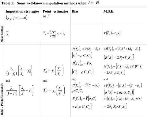
3. Reviewing Existing Imputation Methods and Corresponding Estimators

Some commonly adopted estimators for imputing unknown data values under

non-response sample survey are summarized in Table 1. Assume y_ji denotes

i

th _available

observation for the jth _{imputation strategy.}

Table 1: Some well-known imputation methods when

i



R

'

Imputation strategies



yji;j1,....6



Point estimator

of Y

Bias M.S.E.

Mea

n

Meth

o

d

r

y





 

R i

r i

m y y

r

T 1

 

2

1 y

m S

T

V 

a

to

rs





1 r 1

'

1

   

 



 x f

x f yr

and





r

  

 _

f x y_r

      

r ' '

x x y

TR r

and

r '











y

x

T

 



1 3



' _  _ Y T B _{R I}



Cx CyCx



2

 

4

' 

Y T

B _{R II}



Cx CyCx



2

and

 



1 3



' _  _

Y T B _{P I}

C C 

 





1 3



2 1

'     

y I

R S

T M



R Sx 2RSySx





2

2 

 







2 2

4 3 2 4 '

x y

II

R S R S

T

M     



x yS

S R4

2 

and

 





3



2 1 '

1 



  

 y

I

P S

T M

Pa n d ey e t a l. (2 0 1 5 )

  exp

1 ' 1

' 1                   x x f

x x f y r r r and





exp

1 ' 1

' 1                   x x f

x x f y r r r exp _' ' '          r r r eR x x x x y T and          _'' ' exp x x x x y T r r r eP

 







2

3 1

' _{3 2}

8 x

I

eR C

Y T

B    



1 3



CyCx



4 



 







2



3 4 ' 3 8 x II eR C Y T

B   



x yC C  4 4  and

 

 



2

3 1 ' 8 x I eP C Y T

B   



x yC C  4 

 







2

4 3 ' 8 x II eP C Y T

B   



x yC C  ₄ 4 

 



2

1 ' 4 4 1 y I eR S T

M  





y x



x R S S

S

R   

 3 1

2 2

1 4 



 



2

4 ' 4 4 1 y II eR S T

M  



 



R Sx 4RSySx



2 2 4

3 4



and

 



2

1 ' 4 4 1 y I eP S T

M  



 





R Sx 4RSySx





2 2 3

1 



 



2

4 ' 4 4 1 y II eP S T

M  









R Sx



4R



SySx



2 2 4

3 4

 K a d il a r a n d Cin g i (2 0 0 3 )





1 2 1

2 ' 1       

 x f

x f y r r and





1 '2 1

2 1       

 x f

x f

y_{r r}

2 2 ' ' r r CR x x y T  and 2 2 X x y

T_CP  _r r

 



1 3



'   

Y T

B _{CR I}



3Cx 2CyCx



2 

 







2

4 3 '

3 x

II

CR Y C

T

B    



x yC C  ₄ 2  and

 



1 3



'   

Y T

B _{CP I}



Cx 2CyCx



2 

 







2

4 3 '

3 x

II

CP Y C

T

B   



x yC C  ₄ 2 

 





3 1



2 1 '

4 

    _y I CR S T M



R Sx RSySx





2 2

 



2

4 ' y II CR S T

M  



 



R Sx 4RSySx



2 2 4

3 4

4  



and

 



2

1 ' y I CP S T

M  



 





R Sx RSySx





 2 2

2 1

4

 



2

4 ' y II CP S T

M  



 



R Sx 4RSySx



2 2 4

3 4

4  



4. Proposed Imputation Methods and their Properties

The first proposed method:

1.





2 exp









1

' 1

' ' '

1 8

     

 

   

  

     

  

   

 

  

      

 

R i if f x

x x x x

x f

y

R i if y

y

r r

r r

i

i 



(1)

Using above, the imputation-based estimator of population mean Y is:









_

 

  

   

 

  

      

r r

r r

x x

x x x

x y

T _'

' '

'

) , (

1 2 exp

 



 where

 

,



_{are suitable chosen scalars.} (2)

Theorem 4.1:0.

The estimator, Bias, M.S.E and minimum M.S.E. of '

) , ( 1

T in terms of e₁,e₂ and e₃under design-I and design-IIare obtained as









 _{ }  _{  }

 '

2 '

2 1

'

3 3

) , (

1 4 4 2 2

8 2

1 e e e e e

Y

T _    





2





'2





'

1 2

1 4 3 2 2 2 2 2 3

4ee  ee    e    e

     (3)

 

T _I Y



 





Cx CyCx



B _     2  2 4

8

2 2

3 1 '

) , (

1    

 

 (4)

 















x y x



II Y C C C

T

B '_   2  2₃ 2  2₄ 2 4₄ 8

2

) , (

1      

 

 (5)

 

_ _y  





 







_x  _{y x}



_

I S R S R S S

T

M _      2  4 

4

2 2 2

3 1 2

1 '

) , (

1 (6)

 

_ _y  













_x  _{y x}



_

II S R S R S S

T

M '_ ₄ 2   2  ₃ ₄ 2 2 4 ₄ 4

2

) , (

1 (7)

and





'







₁



_{1 3}



2



2

min ) , (

1 _I Sy

T

M    



    when

x y

RS S  

 2

2   (8)















1 2



2

4 3 2 4 '

4 min

) , (

1 _II Sy

T

M     

 



 

 when





x

y

RS S   

 



4 3

4

2 2

  

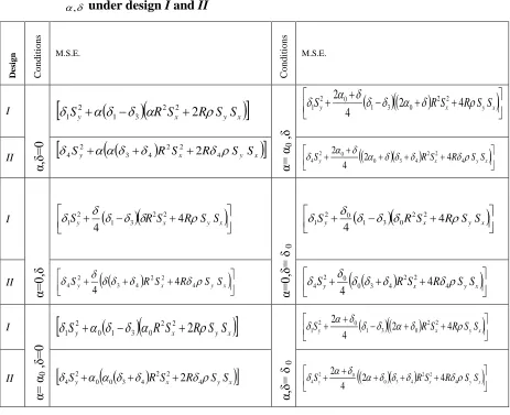
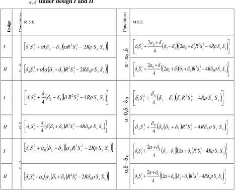
Table 2: M.S.E’s of suggested estimator ' ) , ( 1

T for various parametric settings of



, _{under design} I and II

D

es

ig

n

Co

n

d

it

io

n

s

M.S.E.

Co

n

d

it

io

n

s

M.S.E.

I

α,δ=

0











Sy   R Sx 2RSySx



2 2 3 1 2

1   

α=

α0

,δ











_



  _{  }

 x y x

y RS R S S

S       

 2 4

4

2 2 2

0 3 1 0 2 1

II



 Sy 







 



R Sx R4Sy Sx





2 2 4 3 2

4   2



  



  

 _  _{  }

x y x

y RS R S S

S       

 2 2 ₄

4 3 0 0 2

4 2 4

4 2

I

α=

0,δ









_



 _{  }

x y x

y RS R S S

S     

 4

4

2 2 3 1 2 1

α=

0,δ=

δ 0









_



 _{  }

x y x

y R S R S S

S     

 4

4

2 2 0 3 1 0 2 1

II _ Sy



  R Sx R SySx



_



 2 2 ₄

4 3 2

4 4

4











 

 _{  }

x y x

y R S R S S

S      

 2 2 ₄

4 3 0 0 2

4 4

4

I

α=

α0

,δ=

0











 Sy     R Sx 2RSySx



2 2 0 3 1 0 2

1   

α,δ=

δ 0











_



 _  _{  }

x y x

y RS R S S

S       

 2 4

4

2 2 2

0 3 1 0 2 1

II



 S_y 







 



R2S_x2 R₄S_yS_x





4 3 0 0 2

4   2



  





 

 _  _{  }

x y x

y RS R S S

S       

 2 2 ₄

4 3 0 0 2

4 2 4

4 2

To illustrate the general results, a particular case of the proposed class of estimators '_{ }

, 1

T

is taken letting

   



,



 1,1 in (2), an estimator of population mean is











  

 

   

 

  

      

r r

r r

x x

x x x

x y

T _'

' '

'

exp 2

) 1 , 1 (

1 (10)

Putting

   



,



 1,1 in (4) to (7), the bias and M.S.E. of '

) 1 , 1 ( 1

T under design-I and design-II to the first degree of approximation, respectively is obtained as

 

 







5 4



;

8

3 2

3 1 '

1 , 1

1 _I Y Cx CyCx

T

B     

 

_{ }







_{x y x}



II Y C C C

T

B   2 ₄

4 3 '

1 , 1

1 ₈ 5 4

3 _{ }

 

 

 







3 4



;

4

3 2 2

3 1 2 1 '

1 , 1

1 

 

 _{  }

 y x y x

I S R S R S S

T

M    

 

 

T _II _ Sy 









R Sx  R SySx



_

M ' ₄ 2 3₃ ₄ 2 2 4 ₄

4 3

The second proposed method:

2.





2 exp









1

' 1

' ' '

1 9

     

 

   

  

     

  

   

 

  

      

 

R i if f x

x x x x

x f

y

R i if y

y

n n

n r

i

i 



(11)

Using above, the imputation-based estimator of population mean Y is:









_

 

  

   

 

  

      

n n

n r

x x

x x x

x y

T _'

' '

'

) , (

2 2 exp

 



 where

 

,



_{are suitable chosen scalars.} (12)

Theorem 4.2:

The estimator, Bias, M.S.E. and minimum M.S.E. of '

) , ( 2

T in terms of e₁,e₂ and e₃under design-I and design-II upto first order of approximation are given by









 _{ }  _{  }

 '

3 '

3 1

'

3 3

) , (

2 4 4 2 2

8 2

1 e e e e e

Y

T _    





2





'2





3

' 1 3

1 4 3 2 2 2 2 3

4ee  ee    e    e

     (13)

 



 





x y x



I Y C C C

T

B _     2  2 4

8

2 2

3 2 '

) , (

2    

 

 (14)

 

T _II Y















Cx CyCx



B '_   2  2₃ 2  2₅ 2 4₅ 8

2

) , (

2      

 

 (15)

 

_ _y  





 







_x  _{y x}



_

I S R S R S S

T

M _      2  4 

4

2 2 2

3 2 2

1 '

) , (

2 (16)





_ _y  













_x  _{y x}



_

II S R S R S S

T

M '_ ₄ 2   2  ₃ ₅ 2 2 4 ₅ 4

2

) , (

2 (17)

and











1



2 3



2



2

'

min ) , (

2 I Sy

T

M _      when

x y

RS S  

 2

2   (18)















1 2



2

5 3 2 5 4 '

min ) , (

2 II Sy

T

M _       when





x y

RS S   

 



5 3

5

2 2

  

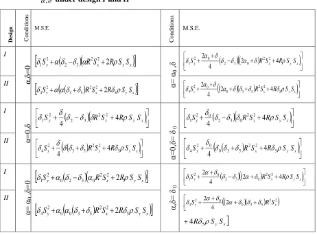
Table 3: M.S.E’s of Suggested estimator ' ) , ( 2

T for various parametric settings of



, _{under design} I and II

D

es

ig

n

Co

n

d

it

io

n

s

M.S.E.

Co

n

d

it

io

n

s

M.S.E.

I

α,δ=

0



Sy 



 





R Sx 2RSySx





2 2 3 2 2

1   

α=

α0

,δ













 



 _  _{  }

x y x

y R S R S S

S       

 2 4

4

2 2 2

0 3 2 0 2 1

II











Sy   RSx R5SySx



2 2 5 3 2

4   2













 

 _  _{  }

x y x

y RS R S S

S       

 5

2 2 5 3 0 0 2

4 2 4

4 2

I

α=

0,δ









_



 _{  }

x y x

y R S R S S

S     

 4

4

2 2 3 2 2 1

α=

0,δ=

δ 0









_



 _{  }

x y x

y R S R S S

S     

 4

4

2 2 0 3 2 0 2 1

II









_



 _{  }

x y x

y RS R S S

S     

 5

2 2 5 3 2

4 4

4











 



 _{  }

x y x

y R S R S S

S      

 2 2 ₅

5 3 0 0 2

4 4

4

I

α=

α0

,δ=

0



Sy 



 





 R Sx 2RSySx





2 2 0 3 2 0 2

1   

α,δ=

δ 0

 







_



 _  _{  }

x y x

y RS R S S

S       

 2 4

4

2 2 2

0 3 2 0 2

1

II











 Sy     R Sx R5SySx



2 2 5 3 0 0 2

4   2

  







 _  _{ } 2 2

5 3 0 0 2

4 2

4 2

x

y RS

S      





x yS

S R₅

4 

To illustrate the general results, a particular case of the proposed class of estimators '_{ }

, 2

T

with its properties is considered. Putting

   



,



 1,1 in (12), an estimator of population mean is









































































n n n

r

x

x

x

x

x

x

y

T

_'

' '

'

exp

2

) 1 , 1 (

2 (20)

Let

   



,



 1,1 in (14) to (17), then the bias and M.S.E. of '

) 1 , 1 ( 2

T under design-I and design-II to the first degree of approximation, respectively is obtained as

 

 

T _I Y







Cx CyCx



B

 

T_{  II} Y







Cx CyCx



B ' ₂ ₃ 2  ' ₃ 5₅ 2 4₅

8 3 ;

4 5 8

3

1 , 1 2 1

, 1

2      

 

 









 

_{ } _ 













_

  

 _{  }

 y x y x _II y x y x

I S RS R S S MT S R S R S S

T

M        5

2 2 5 3 2

4 '

1 , 1 2 2

2 3 2 2 1 '

1 , 1

2 3 4

4 3 ;

4 3

The third proposed method is

3.













     

 

   

  

    

  

     

  

   

 

  

      



 _'

1 '

'

' 1

10

exp

2 1

R i if f

x x

x x x

x f

y

R i if y

y

r r r

r i

i





(21)

Using above, the imputation-based estimator of population mean Y is:









_  

  

    

  

   

 

  

     

 _{' '}'

' ) , (

3 2 exp

x x

x x x

x y

T

r r r

r



 

 where

 

, are suitable chosen scalars.

(22)

Theorem 4.3:

The estimator, Bias, M.S.E. and minimum M.S.E. of '

) , ( 3

T in terms of e₁,e₂ and e3under

design-I and design-II upto first order of approximation are obtainable as









 _{ }  _{  }

 '

2 2

' 1

'

3 3

) , (

3 4 4 2 2

8 2

1 e e e e e

Y

T _













2





'2





'

1 2

1 4 3 2 2 2 2 2 3

4ee  ee    e    e

 (23)

 

T _I Y



 





Cx CyCx



B _     2  2 4

8

2 2

3 1 '

) , (

3    

 

 (24)

 

T _II Y















Cx CyCx



B _         4

2 5 4

' ) , (

3 2 2 2 2 4

8

2  _{     }

 

(25)

 

_ _y  





 







_x  _{y x}



_

I S R S R S S

T

M        



 ₄ 2 4

2 2 2

3 1 2

1 '

) , (

3 (26)

 

T _II _ Sy  













R Sx  R SySx



_

M _        4

2 2 4 3 2

4 '

4 2

4 2

) , (

3 (27)















2



2 3 1 1 min '

) , (

3 y

I S

T

M _      when

x y

RS S  

 2

2   ₍₂₈₎















1 2



2

4 3 2 4 4 min '

) , (

3 _II Sy

T

M _       when

x y

RS S   

 

 2

2

4 3

4

 

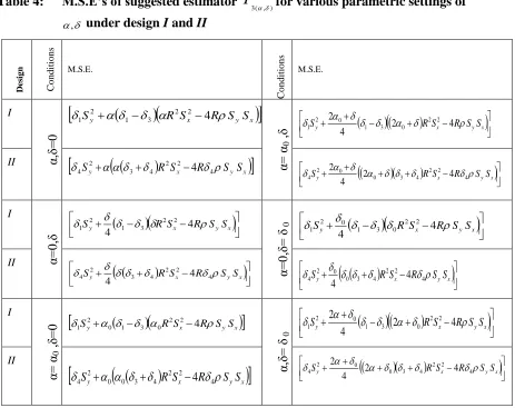
Table 4: M.S.E’s of suggested estimator '

) , ( 3

T

for various parametric settings of



, _{under design} I and II

D

es

ig

n

Co

n

d

it

io

n

s

M.S.E.

Co

n

d

it

io

n

s

M.S.E.

I

α,δ=

0











 Sy   R Sx 4RSySx



2 2 3 1 2

1   

α=

α0

,δ

 







_



  _{  }

 x y x

y RS R S S

S       

 2 4

4

2 2 2

0 3 1 0 2 1

II













x y x

y R S R S S

S    

 4

2 2 4 3 2

4   4



  



  

 _  _{  }

x y x

y RS R S S

S       

 4

2 2 4 3 0 0 2

4 2 4

4 2

I

α=

0,δ

 





_



 _{  }

x y x

y R S R S S

S     

 4

4

2 2 3 1 2 1

α=

0,δ=

δ 0











 

 _{  }

x y x

y R S R S S

S     

 4

4

2 2 0 3 1 0 2 1

II

 





_



 _{  }

x y x

y R S R S S

S      

 4

2 2 4 3 2

4 4

4











 

 _{  }

x y x

y RS R S S

S     

 4

2 2 4 3 0 0 2

4 4

4

I

α=

α0

,δ=

0



Sy    



 R Sx 4RSySx





2

2 0 3 1 0 2

1   

α,δ=

δ 0











_



 _  _{  }

x y x

y RS R S S

S       

 2 4

4

2 2 2

0 3 1 0 2

1

II











 Sy     R Sx R4SySx



2 2 4 3 0 0 2

4   4

  





_



 _  _{  }

x y x

y RS R S S

S       

 4

2 2 4 3 0 0 2

4 2 4

4 2

To illustrate the general result, a particular case of the proposed class of estimators T₃'__,_

is considered. Putting

   

,  1,1 in (22), an estimator of population mean is considered









_

 

  

    

  

   

 

  

     

 _{' '}'

' ) 1 , 1 (

3 2 exp

x x

x x x

x y

T

r r r

r (30)

Let

   

,  1,1 in (24) to (27), we get the bias and M.S.E. of

T

₃₍'_1,1) under design-I and design-II to the first degree of approximation, respectively as

 

 

T _I Y







Cx CyCx



B   4

8

3 2

3 1 '

1 , 1

3    ;B

 

T_{  II} Y





 



Cx 4CyCx



2 3 4 '

4 5

8 3

1 , 1

3   

 

 

_ _y 









_x  _{y x}



_

I S R S R S S

T

M    3 4 

4

3 2 2

3 1 2 1 '

1 , 1

3 ;

 

 

_ _y 









_x  _{y x}



_

II S R S R S S

T

M    4 

2 2 4 3 2

4 '

1 , 1

3 ₄ 3 4

The fourth proposed method is

4.





2 exp









1

' 1

' '

' 1

1 1

     

 

   

  

     

  

   

 

  

      

 

R i if f x

x x x x

x f

y

R i if y

y

n n n

r i

i 



(31)

Using above, the imputation-based estimator of population mean Y is:









__

   

    

  

   

 

  

     

 _{' '}'

' ) , (

4 2 exp

x x

x x x

x y

T

n n n

r



 

 where

 

, _{are suitable chosen scalars.}

(32)

Theorem 4.4:

The estimator, Bias, M.S.E. and minimum M.S.E. of

T

₄'_(,)in terms of e₁,e₂ and e3

under design-I and design-II upto first order of approximation are given as









 _{ }  _{  }

 '

3 3 3

'

3 1

'

) , (

4 4 4 22

8 2

1 e e e ee

Y

T _    









'2





3 2

3 '

3 1 3

1 4 2 2 2 2

4ee  ee   e    e

 (33)

 

T _I Y



 





Cx CyCx



B _     2  2 4

8

2 2

3 2 '

) , (

4    

 

 (34)

 

T _II Y















Cx CyCx



B _         5

2 3 5

' ) , (

4 2 2 2 2 4

8

2  _{     }



 (35)





_ _y  













_x  _{y x}



_

I S R S R S S

T

M _      2  4 

4

2 2 2

3 2 2

1 '

) , (

4 (36)





_ _y  













_x  _{y x}



_

II S R S R S S

T

M _        2 2 ₅

5 3 2

4 '

) , (

4 ₄ 2 4

2

(37)

and











1



2 3



2



2

min '

) , (

4 _I Sy

T

M _      when

x y

S S

R 

 2

2   ₍₃₈

 











1 2



2

5 3 2 5 4 '

min ) , (

4 _II Sy

T

M _       when

x y

S S

R  

 



5 3

5

2 2

 

Table 5: M.S.E’s of suggested estimator ' ) , ( 4

T for various parametric settings of



, _{under design} I and II

D

es

ig

n

Co

n

d

it

io

n

s

M.S.E.

Co

n

d

it

io

n

s

M.S.E.

I

α,δ=

0











 Sy    R Sx 2RSySx



2

2 3 2 2

1   

α=

α0

,δ











_



 _  _{  }

x y x

y RS R S S

S       

 2 4

4

2 2 2

0 3 2 0 2 1

II



_4S2_y







₃₅



_R2_Sx2_2R₅_SySx















  

 _  _{  }

x y x

y RS R S S

S       

 5

2 2 5 3 0 0 2

4 2 4

4 2

I

α=

0,δ









_



 _{  }

x y x

y R S R S S

S     

 4

4

2 2 3 2 2 1

α=

0,δ=

δ 0











 

 _{  }

x y x

y R S R S S

S     

 4

4

2 2 0 3 2 0 2 1

II _ Sy







 



R Sx R SySx



_



 5

2 2 5 3 2

4 4

4











 

 _{  }

x y x

y R S R S S

S      

 2 2 ₅

5 3 0 0 2

4 4

4

I

α=

α0

,δ=

0











 Sy     R Sx 2RSySx



2 2 0 3 2 0 2

1   

α,δ=

δ 0











_



 _  _{  }

x y x

y R S R S S

S       

 2 4

4

2 2 2

0 3

2 0 2

1

II



_4S2_y₀



₀



₃₅



_R2_Sx2_2R₅_SySx















  

 _  _{  }

x y x

y RS R S S

S       

 5

2 2 5 3 0 0 2

4 2 4

4 2

To illustrate the general result, a particular case of the proposed class of estimators T₄'_(,) is considered. Putting

   

,  1,1 _{in (32), an estimator of population mean is}









_

 

  

   

 

   

 

  

     

 _{' '}'

'

exp 2

) 1 , 1 ( 4

x x

x x x

x y

T

n n n

r (40)

Putting

   

,  1,1 in (34) to (37), the bias and M.S.E. of

T

₄₍'_1,1)under design-I and design-II to the first degree of approximation, respectively is given as:

 

 







4



;

8

3 2

3 2 '

1 , 1

4 x y x

I Y C C C

T

B     

 

_{ }







_{x y x}



II Y C C C

T

B   2 ₅

3 5 '

1 , 1

4 ₈ 5 4

3 _{ }

 

 

 







3 4



;

4

3 2 2

3 2 2 1 '

1 , 1

4 

 

 _{  }

 _{y x y x}

I S R S R S S

T

M    

 

 

_ _y 









_x  _{y x}



_

II S R S R S S

T

M    2 2 ₅ 

5 3 2

4 '

1 , 1

4 ₄ 3 4

5. Comparison of Estimators

Conditions for superiority among the proposed class of estimators are described as under (for proof, see Appendix II):

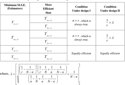
Table 6: Efficiency Comparisons within Proposed estimators

Minimum M.S.E. (Estimators)

More Efficient

than

Condition Under design I

Condition Under design II

 

'

, 1

T  

'

, 2

T

r

n , which is

always true. _r 

1

 

'

, 4

T

 

'

, 3

T  

'

, 2

T

r

n , which is

always true. _r 

1

 

'

, 4

T

 

'

, 1

T '_{ }

, 3

T

Equally efficient Equally efficient

 

'

, 2

T '_{ }

, 4

T

where,

    

 

    

 

  

  

 

   

   

 

       

 

 

 _'

' '

' '

2

'

1 1

1 1 1

1 1 1 1 1

1

n N n

N n N n

n N n N r n N r 

Conditions under which the proposed estimators are more efficient than the contemporary estimators are summarized as under (for proof, see Appendix II):

Table 7: Efficiency Comparisons among Proposed and Existing Estimators

M.S.E Under design I Under design II

Estimator

More efficient

than

Condition

   

 

 

x y

S S

Condition

   

 

 

x y

S S

'

R

T either, _{N n}

N n r

   

2 



3 _4



'

eP

T

either,

n N

N n r

   

2

or,

2

R

  





4 4 3

2  

  R

'

CR

T either, N n

N n r

   

2

or,2 4R



Rk







4 4 3

2 

 

  R

'

CP

T R











Rk





 



3 1

2 1

2 4

 

 







4 4 3

2 

 

  R

   

' '

, 4 ,

2 T 

T 

'

R

T







 

R kR



 

 2

3 2

3 1 2

 

  













4 3 4 2

5 5 3 2

2















  R k 

'

P

T











R



kR



 

 2

3 2

3 1 2

 

  













4 3 4 2

5 5 3 2

2  

  

   R k 

'

eR

T



 

_ 



 _

 

4

1 3 1 3 2

2 R

k

R _{ } 

 

 



2



R 4k



3₄ 4



R 5

5 3

2   

   

'

eP

T R











kR



   

3 2

3 1 2

4   

 



2



R 4k



3₄ 4



R 5

5 3

2   

   

'

CR

T _R _



Rk



  

3 2

3 1 2 4

 

 









k





R



R

4 3 4 2 5

5 3

2 4   

  

    

'

CP

T _R _



Rk





  

3 2

2 1 2 4

 

 





2



R



4k



3 4



R



5 5 3

2 4   

  

    

6. Illustrative Examples

Population A [Source: Kadilar and Cingi (2006)]: Y represents apple production and X

represents number of apple trees. Other related information to population are:

N =106 n= 20 Y = 2212.59 X = 27421.70



=0.86 Sy=11551.53

y

C =5.22 S_x=57460.61 C_x=2.10 n'= 60 r=15

Population B [Source: Koyuncu and Kadilar (2009)]:Y is number of teachers and X is number of students. Other related information to population are:

N

=923 n= 180 Y = 436.4345 X = 11440.498 =0.9543

y

The population C [Source: Murthy (1967)]: Y is area under winter paddy and X is corresponding geographical area. The following data is based on the given population:

N

=108 n= 30 Y = 172.3704 X = 461.3981 =0.7896

y

S =134.3567 C_y=0.7795 S_x=318.5022 C_x=0.6903 n'= 70 r=20

The Percentage Relative Efficiencies (P.R.E.’s) of the estimatorsTm,TR,TeR,TCR,

, 2,

1 ,T

T ,T_{3,}and T_{4,} for the population A, population B, and population C with respect to Tmunder two-phase sampling scheme is computed by using the following

formula





 

X j I or II MSE

T MSE T

PRE

j m

m  

  

 

 100;

(*)

*, (41)

where (*) represents the respective estimator. The results are summarized in Table 8.

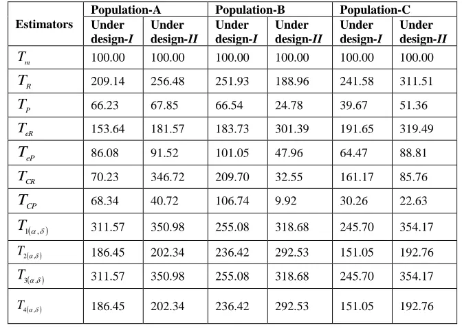
Table 8: PREs of various estimators w.r.to Tmunder Two-Phase Sampling design

Estimators

Population-A Population-B Population-C Under

design-I

Under design-II

Under design-I

Under design-II

Under design-I

Under design-II

m

T 100.00 100.00 100.00 100.00 100.00 100.00

R

T 209.14 256.48 251.93 188.96 241.58 311.51

P

T 66.23 67.85 66.54 24.78 39.67 51.36

eR

T 153.64 181.57 183.73 301.39 191.65 319.49

eP

T 86.08 91.52 101.05 47.96 64.47 88.81

CR

T 70.23 346.72 209.70 32.55 161.17 85.76

CP

T 68.34 40.72 106.74 9.92 30.26 22.63

, 1

T 311.57 350.98 255.08 318.68 245.70 354.17

 ,

2

T 186.45 202.34 236.42 292.53 151.05 192.76

 ,

3

T 311.57 350.98 255.08 318.68 245.70 354.17

,

4

T 186.45 202.34 236.42 292.53 151.05 192.76

7. Conclusions

To sum up, analytic discussion based on some contemporary and some proposed imputed mean estimates for unit non response in field substitution, is now carried out. Data from three different studies, comprising of positively related auxiliary variable and study variable have been selected for the purpose of illustration. Table 6 shows theoretic conditions for efficiency comparisons within proposed estimators. On the basis of corresponding minimum M.S.E.’s, the proposed estimators _{ } '_{ }

, 3 '

,

1 ,T 

T are found to be

equally efficient. Similarly, the proposed estimators _{ } '_{ } , 4 '

,

2 ,T 

T are also found to be

equally efficient. Overall, the proposed estimators T₁'_{,}T₃'_{,} are evidenced to be better than the proposed estimator '_{ } '_{ }

, 4 ,

2 T 

T  and the entire considered existing

estimator.

Conditions of the four proposed estimators being more efficient, under each design as compared with ratio, product estimator, exponential ratio, exponential product, combined ratio and combined product estimators are shown in table 7. Tables 7 distinctly indicates conditions for all the four proposed estimators to be more efficient (and hence superior) than the six existing estimators considered in this paper, under both designs.

Table 8 gives insight on the Percentage Relative Efficiency (P.R.E.) of various estimators under Two-Phase Sampling w.r.to. Tm. Three populations from classical statistical

literature are considered for comparison, each of which consistently shows that the proposed estimators are more competent for imputation in practice. We conclude that our proposed estimators '_{ }

, 1

T and '_{ }

, 3

T outperform all other contemporary estimators considered, under each design. It is evident that under each design the proposed estimators '_{ }

, 1

T and '_{ }

, 3

T are equally efficient and the proposed estimators '_{ } , 2

T and

  '

, 4

T are also equally efficient. Also, proposed estimators '_{ } , 1

T and '_{ }

, 3

T perform better

than the proposed estimators '_{ } , 2

T and '_{ }

, 4

T . The present paper is therefore an important

contribution for the practitioners in the area of missing data analysis as it offers improved estimators than the existing ones for imputing lost or missing data.

Acknowledgements

Part of the work of the first author is supported by R& D Grant from University of Delhi. The authors are grateful to an associate editor and the referees for their constructive suggestions which has considerably improved the manuscript.

References

1. Kadilar, C. and Cingi, H. (2006).