Improved Ratio-type Estimators of Population Mean In Ranked Set Sampling Using Two Concomitant Variables

in Ranked Set Sampling Using Two Concomitant Variables

Lakhkar Khan

Department of Statistics, Quaid-i-Azam University, Islamabad, Pakistan [email protected]

Javid Shabbir

Department of Statistics, Quaid-i-Azam University, Islamabad, Pakistan [email protected]

Abstract

In this paper, we propose an efficient class of ratio-in-exponential-type estimators with two concomitant variables using Ranked Set Sampling (RSS) scheme which improves the available estimators. The biases and mean square errors (MSEs) of the proposed estimators are obtained up to first degree approximation. Comparisons among the proposed and competitor estimators are made both theoretically and through simulation study. It turned out that when the variable of interest and the concomitant variables jointly followed a trivariate Gamma distribution, the proposed class of estimators dominates all other competitor estimators.

Keywords: Ranked set sampling, MSE, Bias, Concomitant variables. Mathematics subject classification 62D05.

1. Introduction

Ranked set sampling (RSS) is a sampling technique which is used to reduce cost and increase efficiency in that situation where the measurement of survey variable is costly and time consuming, but it can be ranked easily at no cost or at very little cost. The technique of RSS was first introduced by Mclntyre (1952) to increase efficiency of the estimator of the population mean. The general method of a RSS can be described as follows: First, m subsamples, each of size m, are drawn at random from a population. Next, for each sub sample, the elements in the subsample are ranked relating to the concomitant variables and then one and only one element of the subsample ranked is measured. The procedure produces a sample of n measurement of independent order statistics.

that it has less variance as compared to usual ratio estimator in SRS. Khan and Shabbir (2015) suggested a class of Hartley-Ross type unbiased estimator in RSS. Khan and Shabbir (2016) have also suggested Hartley-Ross type unbiased estimators in RSS and stratified ranked set sampling (SRSS). Khan et al. (2016) proposed unbiased ratio estimator of finite population mean in SRSS.

Munoz and Rueda (2009) used relative bias (RB) and the relative root mean square error (RRMSE), for the comparison of different estimators. For the more detail see Chambers and Dunstan (1986), Rao et al. (1990), Silva and Skinner (1995) and Harms and Duchesne (2006).

In this article, we investigate the properties of the usual mean estimator in RSS and propose an efficient class of the ratio-in-exponential type estimators using two concomitant variables under RSS scheme.

2. Ranked set sampling procedure with two concomitant variables

In ranked set sampling m independent random samples each of size m are chosen and the items in each sample are selected with equal probability and without replacement from a finite population of size N. The items of each random sample are ranked with respect to the characteristic of the study variable or concomitant variable. Let Y be the study variable and X and Z are the two concomitant variables. Then randomly select 2

m trivariate sample elements from the population and allocate them into m sets, each of size m. Each sample is ranked with respect to one of the concomitant variable X or Z. Here, ranking is done on the basis of the concomitant variable X. An actual measurement from the first sample is then taken on the item with the smallest rank of X, together with variable Y and Z associated with smallest rank of X. From the second sample of size m, the variables Y and Z associated with the second smallest rank of X are measured. By this way, this procedure is continued until, the Y and Z values associated with the highest rank of X are measured from the th

m sample. This completes one cycle of sampling process. The procedure is repeated r times to obtain a sample of size nmr items. Thus in a RSS scheme, a total of m r2 items have been drawn from the population and only mr of them are selected for analysis. To estimate the population mean,

 

Y , in RSS using ratio-type estimator with two concomitant variables, the procedure of selecting n ranked set samples can be summarized as follows:

Step 1: Randomly select 2

m _{trivariate sample items from the population.}

Step 2: Allocate these m2 _{items into m sets, each of size}m .

Step3: Each set is ranked with respect to the concomitant variable X.

Step 4: Select the ith ranked item from the ith



i1, 2,...,m



set for actual magnitude.

The usual RSS mean estimator y_(RSS) and its variance, are given by

( ) [ : ] ,

1 1

1 r m

RSS i m j

j i

y y

mr  





(1)





2 2 2

( ) [ ]

( _RSS ) _{y y} , V y Y C W

(2)

where [ ]2 ₂ 2 2[ : ] 1

1

,

m

y y i m

i

W

m rY 





 y i m[ : ]



y i m[ : ]Y



,

1 mr

 _{ } _

  and Cyis the coefficient of

variation of y. The value of _{y i m[ : ]} depends on order statistics from some specific distribution (see Arnold et al, 1992).

3. Proposed class of estimators in RSS

We propose a class of ratio-in-exponential type estimators having two concomitant variables X and Z in RSS as

(3)

where

[ ] [ : ] ,

1 1

1 r m

rss i m j

j i

y y

mr  





, _{( ) ( : ) ,}

1 1

1 r m

rss i m j

j i

x x

mr  





, _{[ ] [ : ] ,}

1 1

1 r m

rss i m j

j i

z z

mr  





1

 and ₂ are unknown constant whose values are to be determined so that MSE of

( )

G RSS

y is minimized and k is a scalar quantity which can take 0 or 1 values. Also X and Zare the population means of X and Z respectively.

To find the bias and MSE of the estimators, we define the following error terms: Lety_[rss]Y



1e₀



, x_(rss) X



1e₁



, z_[rss]Z



1e₂



Such thatE e

 

_p 0, (p=0, 1, 2,), and

 

2 2 2

0 y [ ]y 200,

E e C W V E e

 

₁2 C_x2W_{[ ]x}2 V₀₂₀, E e

 

₂2 C_z2 W_{[ ]}2_z V₀₀₂,

 

0 1 yx (yx) 100,

E e e C W V E e e



_{0 2}



C_yzW_[yz]V₁₀₁, E e e

 

_{1 2} C_xzW_(xz) V₀₁₁,

2 2

[ ] ₂ 2 [ : ]

1

1 m

y y i m

i

W

m rY 





 , _{( )}2 _{2 2} 2_{( : )}

1

1 m

x x i m

i

W

m rX 





 , _{[ ]}2 _{2 2} 2_{[ : ]}

1

1 m

z z i m

i

W

m rZ 







2

( ) ₂ ( : )

1

1 m

yx yx i m

i

W

m rY X 





 , _{[ ]} 2_{[ : ]}

2

1

1 m

yz yz i m

i

W

m rY Z 





 , _{( )} 2_{( : )}

2

1

1 m

xz xz i m

i

W

m r X Z 











[ : ] [ : ]

y i m y i m Y

   , x i m( : ) 



x i m( : )Y



, z i m[ : ]



z i m[ : ]Y









( : ) [ : ] ( : )

yx i m y i m Y x i m X

    , _{yz i m[ : ]}



_{y i m[ : ]}Y



_{z i m[ : ]}Z



,







( : ) ( : ) [ : ]

xz i m x i m X z i m Z

    .

1 2

( ) [ ]

( ) [ ]

( ) [ ] ( ) [ ]

exp rss (1 ) exp rss

G RSS rss

rss rss rss rss

X x Z z

X Z

y y k k

x z X x Z z

Here C_yx _yxC C_{x y}, C_yz _yzC C_{y z}, C_xz _xzC C_{x z}, where C_x,C_y and C_z are the coefficients of variation of X, Y and Z respectively. The values of _{x i m[ : ]} and _{z i m[ : ]} depend on order statistics from some specific distributions.

In terms of e s, up to first order of approximation, we have













2 2

( ) 0 1 1 1 0 1 1 1 1 2 2 2 2 2

2 2

1 1 2 2

1 1

1 1 1 1

2 2

1 3 1 3

1 1 1 ,

2 8 2 8

G RSS

y Y e e e e e e e

k e e k e e

            _      _{ }    _       _{ } _{ }  _{ }       _{   }   or













































2

0 1 1 2 2 1 1 1 1

2

( ) 2 2 2 2 1 0 1 2 0 2

1 2 1 2 1 2

1 1 1

2 1 2 4 3 4 1

2 2 8

1 1 1

( ) (1 ) 4 1 4 1 2 1 2 .

8 2 2

1

(1 ) 2 2

G RSS

e k e k e k e

y Y Y k e k e e k e e

k k e e

               _{        }          _          _            (4)

The bias ofy_{G RSS( )}, is given by









































1 1 1 020 2 2 2 002

( )

1 110 2 101 1 2 1 2 011

1 1

4 3 4 1 (1 ) 4 1 4 1

8 8

.

1 1 1

2 1 2 (1 ) 2

2 2 2

G RSS

k V k V

Bias y Y

k V k V k k V

             _{       }       _{        }      (5)

Taking square of Eq. (4) and then expectations, the MSE ofy_{G RSS( )}, is given by



























2 2

200 1 020 2 002 1 110

2

( )

2 101 1 2 011

1 1

2 1 2 2

4 4

. 1

1 2 2 1 2

2

G RSS

V k V k V k V

MSE y Y

k V k k V

       _{      }       _{      }      (6)

The optimum values of 1 and 2 are

2

1( ) 2

2 ( ) (1 )

2 (1 )

y yx xz yz x xz

opt x xz C kC C                (7) and 2

2( ) 2

2 ( ) (1 ) (1 )

. 2 (1 )

y yx xz yz z xz opt

x xz

C k C

It is remarked that for different values of ₁ and ₂ in Eq (3), we can get various exponential ratio-type estimators from the proposed family of estimatorsy_{G RSS( )}. Some are given below as:

(i) For ₁1,₂ 0 and k 0, we get

[ ]

1( ) [ ]

( ) [ ]

exp rss

RSS rss

rss rss

Z z X

y y

x Z z

    

 _ _ _ _



 

  (9)

The bias and MSE of y_1(RSS),are given respectively



1( )



020 002 110 101 011

1 1 1

8 2 2

RSS

Bias y Y V_  V V  V  V _

  (10)

and





2

1( ) 020 020 002 110 101 011

1

2 .

4

RSS

MSE y Y _V V  V  V V V _

  (11)

(ii) For ₁0, ₂ 1 and k 1, we get

( )

2( ) [ ]

[ ] ( )

exp rss

RSS rss

rss rss

X x

Z

y y

z X x

 

  

 _ _ _ _



    (12)

The bias and MSE of y_2(RSS), are given respectively



2( )



020 002 110 101 011

3 1 1

8 2 2

RSS

Bias y Y_ V V  V  V V _

  (13)

and





2

2( ) 200 020 002 110 101 011

1

2 .

4

RSS

MSE y Y _V  V V V  V V _

  (14)

(iii) For ₁1,₂ 0and k 1, we get

( )

3( ) [ ]

( ) ( )

exp rss

RSS rss

rss rss

X x

X

y y

x X x

    

 _ _ _ _



    (15)

The bias and MSE of y_3(RSS), are given respectively



3( )



020 110

15 3

8 2

RSS

Bias y Y_ V  V _

  (16)

and





2

3( ) 200 020 110

9

3 .

4

RSS

MSE y Y _V  V  V _

  (17)

(iv) For 10,2 1and k 0, we get

[ ]

4( ) [ ]

[ ] [ ]

exp rss

RSS rss

rss rss

Z z Z

y y

z Z z

    

 _ _ _ _



The bias and MSE of y_4(RSS), are given respectively



4( )



002 101

13 3

8 2

RSS

Bias y Y_ V  V _

  (19)

and





2

4( ) 200 002 101

9

3 .

4

RSS

MSE y Y _V  V  V _

  (20)

(v) For k 1, Eq. (3) becomes

1 2

( )

5( ) [ ]

( ) [ ] ( )

exp rss

RSS rss

rss rss rss

X x

X Z

y y

x z X x

 

      

 _ _ _ _ _ _



 

    (21)

The bias and MSE of y_5(RSS), are given respectively





















2

1 1 020 2 2 002

5( )

1 101 2 101 2 1 011

1 1

4 8 3 1

8 2

1 1

1 2 1 2

2 2

RSS

V V

Bias y Y

V V V

         _{   }       _{    }   

  ₍₂₂₎

and

















2 ₂

2 _{200 1 020 2 002 1 110}

5( )

2 101 2 1 011

1

1 2 1 2

4 .

2 1 2

RSS

V V V V

MSE y Y

V V        _{    }     _{ }     

  ₍₂₃₎

The optimum values of ₁ and ₂ are













2 *

1( ) 2

2 1

2 1

y yx xz yz x xz opt x xz C C C            (24) and









*

2( ) 2 .

2 1

y yx xz yz opt z xz C C         (25)

By putting the optimum values of ₁ and ₂ in Eq. (22) and Eq. (23), we get the minimum bias and MSE ofy_5(RSS) respectively as







2 2



5( ) _min ( )

1 8

RSS x x

Bias y  Y C W (26)

and









2

2

2 2 2

5( ) _min 200

1

. (1 )

y

yx xz

RSS x xz

C

MSE Y Y V C   

(vi) For k 0, Eq.(3) becomes

1 2

[ ]

6( ) [ ]

( ) [ ] [ ]

exp rss

RSS rss

rss rss rss

Z z

X Z

y y

x z Z z

 

      

 _  _{ } _ _ _



   

  (28)

The bias and MSE ofy_6(RSS), are given respectively

















2

1 1 020 2 2 002

6( )

1 110 2 101 1 2 011

1 1

1 4 8 1

2 8

( )

1 1

1 2 1 2

2 2

RSS

V V

Bias y Y

V V V

         _{   }       _{    }   

  ₍₂₉₎

and













2 2

2 _{200 1 020 2 002 1 110}

6( )

2 101 1 2 011

1

1 2 2

4 .

1 2 2

RSS

V V V V

MSE y Y

V V        _{   }     _{ }     

  ₍₃₀₎

The optimum values of ₁and ₂









**

1( ) 2

2 1

y yx xz yz opt x xz C C         (31) and













2 **

2( ) 2

2 1

.

2 1

y yx xz yz z xz opt z xz C C C            (32)

By putting Eqs.(31) and (32) in Eqs.(29) and (30), the minimum bias and MSE of y_6(RSS), are given respectively







2 2



6( ) _min [ ]

1 8

RSS z z

Bias y  Y C W (33)

and









2

2

2 2 2

6( ) _min 200

1

. (1 )

y

yz xz

RSS z xz

C

MSE Y Y V C   

       _  _     (34)

4. Efficiency Comparison

We obtain the conditions under which the proposed estimators are more efficient than the usual RSS mean estimator.

(i) Comparison: By Eq.(2) and Eq.(11)



1(RSS)





(RSS)



MSE y MSE y , if

020 002

110 101 011

1

4 ₁

2

V V

V V V



(ii) Comparison: By Eq.(2) and Eq.(14)



2(RSS)





(RSS)



MSE y MSE y , if

020 002

110 101 011

1

4 ₁

2

V V

V V V





 

(iii) Comparison: By Eq.(2) and Eq.(17)



3(RSS)





(RSS)



MSE y MSE y if

3

1 4

x y yx

C C  

(iv) Comparison: By Eq.(2) and Eq.(20)



4(RSS)





(RSS)



MSE y MSE y , if

3

1 4

z y yz

C C  

(v) Comparison: By Eq.(2) and Eq.(27)



5(RSS)



_min



(RSS)



MSE y MSE y , if





2

0

yx xz

  

(vi) Comparison: By Eq.(2) and Eq.(34)



6(RSS)



_min



(RSS)



MSE y MSE y , if





2

0

yz xz

  

5. Simulation Study

and r. The results are shown in Tables 1, 2, 3 and 4. The findings indicate that with increase in sample size, MSEs, RB, RRMSEs decrease which are expected results. We used the following expressions to obtain the MSE, RB, RRMSE and PRE:





20000

( ) ( )

1

1 1

( )

20000

G RSS G RSS i

i

RB y y Y

Y 

 

 _  _





 , G1, 2,..., 6





1

20000 ₂

2

( ) ( )

1

1 1

( )

20000

G RSS G RSS i

i

RRMSE y y Y

Y 

 

 _  _





 ,





20000

2

( ) ( )

1

1

( )

20000

G RSS G RSS i i

MSE y y Y







 and







(( ))



100

RSS

G RSS

MSE y PRE

MSE y

  , G1, 2,..., 6

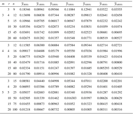
Table 1: The Simulated MSE of Different Estimators

m r n (RSS) 1(RSS) 2(RSS) 3(RSS) 4(RSS) 5(RSS) 6(RSS) 3 9 0.18346 0.08961 0.09566 0.11084 0.12941 0.03522 0.03555

3 4 12 0.13698 0.06838 0.07344 0.08287 0.09813 0.02641 0.02658

5 15 0.10966 0.05705 0.06017 0.06947 0.07879 0.02232 0.02242

10 30 0.05356 0.02673 0.02873 0.03234 0.03831 0.01059 0.01074

15 45 0.03691 0.01742 0.01899 0.02052 0.02523 0.00681 0.00695

20 60 0.02675 0.01282 0.01357 0.01548 0.01771 0.00519 0.00527

3 12 0.11585 0.06300 0.06884 0.07584 0.09344 0.02714 0.02721

4 4 16 0.09017 0.04688 0.05179 0.05550 0.07036 0.01984 0.01996

5 20 0.06775 0.03629 0.03940 0.04408 0.05339 0.01623 0.01634

10 40 0.03479 0.01716 0.01885 0.02091 0.02596 0.00791 0.00800

15 60 0.02334 0.01151 0.01247 0.01397 0.01685 0.005293 0.00529

20 80 0.01790 0.00914 0.00996 0.01082 0.01328 0.00408 0.00410

3 15 0.08581 0.04440 0.04998 0.05344 0.07011 0.02200 0.02201

4 20 0.06093 0.03386 0.03789 0.04082 0.05294 0.01601 0.01605

5 5 25 0.05037 0.02683 0.02881 0.03340 0.03936 0.01287 0.01292

10 50 0.02505 0.01339 0.01462 0.016303 0.01997 0.00626 0.00629

15 75 0.01655 0.00873 0.00963 0.01052 0.01323 0.00415 0.00418

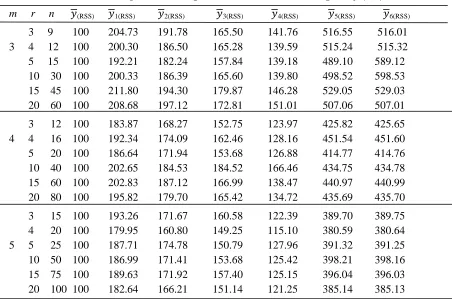
Table 2: The Percentage RE of Proposed Estimators with respect (RSS)

m r n (RSS) 1(RSS) 2(RSS) 3(RSS) 4(RSS) 5(RSS) 6(RSS)

3 9 100 204.73 191.78 165.50 141.76 516.55 516.01 3 4 12 100 200.30 186.50 165.28 139.59 515.24 515.32 5 15 100 192.21 182.24 157.84 139.18 489.10 589.12 10 30 100 200.33 186.39 165.60 139.80 498.52 598.53 15 45 100 211.80 194.30 179.87 146.28 529.05 529.03 20 60 100 208.68 197.12 172.81 151.01 507.06 507.01

3 12 100 183.87 168.27 152.75 123.97 425.82 425.65 4 4 16 100 192.34 174.09 162.46 128.16 451.54 451.60 5 20 100 186.64 171.94 153.68 126.88 414.77 414.76 10 40 100 202.65 184.53 184.52 166.46 434.75 434.78 15 60 100 202.83 187.12 166.99 138.47 440.97 440.99 20 80 100 195.82 179.70 165.42 134.72 435.69 435.70

3 15 100 193.26 171.67 160.58 122.39 389.70 389.75 4 20 100 179.95 160.80 149.25 115.10 380.59 380.64 5 5 25 100 187.71 174.78 150.79 127.96 391.32 391.25 10 50 100 186.99 171.41 153.68 125.42 398.21 398.16 15 75 100 189.63 171.92 157.40 125.15 396.04 396.03 20 100 100 182.64 166.21 151.14 121.25 385.14 385.13

Table 3: The Simulated Percentage RRMSE of Different Estimators

m r n (RSS) 1(RSS) 2(RSS) 3(RSS) 4(RSS) 5(RSS) 6(RSS)

Table 4: The Simulated Percentage RB of Different Estimators

m r n (RSS) 1(RSS) 2(RSS) 3(RSS) 4(RSS) 5(RSS) 6(RSS)

3 9 0.20 1.99 1.73 1.81 1.56 0.51 0.52 3 4 12 0.14 1.62 1.12 1.56 1.82 0.18 0.16 5 15 0.08 1.43 1.30 1.43 1.76 0.08 0.07 10 30 -0.07 0.68 0.56 0.68 0.85 -0.05 -0.04 15 45 -0.05 0.29 0.20 0.29 0.45 -0.03 -0.03 20 60 -0.02 0.23 0.26 0.23 0.24 -0.01 -0.01 3 12 -0.76 1.99 1.86 1.99 1.33 0.20 0.19 4 4 16 -0.03 1.58 1.41 1.58 1.92 0.36 0.35 5 20 0.09 0.95 0.88 0.95 1.16 0.20 0.18 10 40 -0.02 0.53 0.48 0.53 0.65 0.10 0.11 15 60 -0.04 0.26 0.31 0.26 0.25 0.05 0.05 20 80 -0.02 0.35 0.28 0.35 0.44 0.04 0.03 3 15 0.24 0.95 0.80 0.95 0.83 0.06 0.06 5 4 20 -0.21 0.83 0.82 0.82 0.96 0.07 0.05 5 25 -0.17 0.71 0.73 0.71 0.79 0.14 0.13 10 50 -0.09 0.32 0.27 0.32 0.41 -0.02 -0.02 15 75 0.02 0.23 0.20 0.23 0.29 0.03 0.01 20 100 -0.01 0.12 0.11 0.12 0.16 0.00 0.00

6. Conclusion

In Tables 1 and 3, we see that the proposed ratio-in-exponential type estimatorsy_{G RSS( )}, have less MSE and RRMSE values as compared toy_(RSS). Also, MSE and RRMSE decrease with increase in the sample size. The simulation result of Table 4 indicate that the proposed estimators have reasonable biases, since the values of percentage RB are all less than 2% in absolute terms. Also, the value of percentage RB decreases with increase in sample size nmr. _{So, we conclude that the proposed ratio-in-exponential type} estimators are preferable than the usual mean estimator under RSS scheme.

Acknowledgement

The authors wish to thank the cheif editor and the referees for their valuable suggestions regarding improvenment of the paper.

References

1. Arnold, B. C., Balakrishnan, N. and Nagaraja, H. N. (1992). A First Course in Order Statistics. Vol. 54, Siam.

3. Harms, T and Duchesne, P. (2006). On calibration estimation for quantile. Survey Methodology, 32, 37-52.

4. Khan, L. and Shabbir, J. (2015). A class of Hartley-Ross type unbiased estimators for popula- tion mean using ranked set sampling. Hacettepe Journal of Mathematics and Statistics, Doi:10.15672/HJMS.20156210579, in Press.

5. Khan, L. and Shabbir, J. (2016). Hartley-Ross type unbiased estimators for population mean using ranked set sampling and stratified ranked set sampling. North Carolina Journal of Mathematics and Statistics, Vol.2, 10-22.

6. Khan, L. Shabbir, J. and Gupta, S. (2016). Unbiased ratio estimators of the mean in stratified ranked set sampling. Hacettepe Journal of Mathematics and Statistics, Doi:10.15672/HJMS.20156210579, in Press.

7. Mclntyre, G. (1952). A method for unbiased selective sampling using ranked sets. Crop and Pasture Science, 3(4):385-390.

8. Munoz, J. F. and Rueda, M. (2009). New imputation method for missing data using quantiles. Journal of Computational and Applied Mathematics, 232, 305-317.

9. Rao, J.N.K. Kovar, J.G. and Mantel, H.J. (1990). On estimating distribution function and quantiles from survey data using auxiliary information. Biometrika, 77, 365-375.

10. Samawi, H. M. and Muttlak, H. A. (1996). Estimation of ratio using ranked set sampling. Biometrical Journal, 38 (6), 753-764.

11. Silva, P.L.D. and Skinner, C.J. (1995). Estimating distribution function with auxiliary information using poststratification. Journal of Official Statistics, 11, 277-294.13

12. Singh, H. P., Tailor, R. and Singh, S. (2014). General procedure for estimating the population mean using ranked set sampling. Journal of Statistical Computation and Simulation, 84(5):931-945.

13. Stokes, S. L. (1977). Ranked set sampling with concomitant variables. Communication in Statistics: Theory and Methods, 6(12): 1207-1211.