www.nonlin-processes-geophys.net/21/357/2014/ doi:10.5194/npg-21-357-2014
© Author(s) 2014. CC Attribution 3.0 License.
Nonlinear Processes
in Geophysics
Mitigation of coupled model biases induced by dynamical core
misfitting through parameter optimization: simulation with a simple
pycnocline prediction model
G.-J. Han1, X.-F. Zhang1, S. Zhang2, X.-R. Wu1, and Z. Liu3,4
1Key Laboratory of Marine Environmental Information Technology, State Oceanic Administration,
National Marine Data and Information Service, Tianjin, China
2GFDL/NOAA, Princeton University, Princeton, NJ, USA
3Nelson Institute Center for Climatic Research and the Department of Atmospheric and Oceanic Sciences,
University of Wisconsin-Madison, Madison, WS, USA
4Laboratory for Climate, Ocean and Atmosphere Studies, Peking University, Beijing, China
Correspondence to: G.-J. Han ([email protected])
Received: 17 September 2013 – Revised: 13 January 2014 – Accepted: 25 January 2014 – Published: 7 March 2014
Abstract. Imperfect dynamical core is an important source of model biases that adversely impact on the model simu-lation and predictability of a coupled system. With a sim-ple pycnocline prediction model, in this study, we show the mitigation of model biases through parameter optimization when the assimilation model consists of a “biased” time-differencing. Here, the “biased” time-differencing is defined by a different time-differencing scheme from the “truth” model that is used to produce “observations”, which gen-erates different mean values, climatology and variability of the assimilation model from the “truth” model. A series of assimilation experiments is performed to explore the impact of parameter optimization on model bias mitigation and cli-mate estimation, as well as the role of different media pa-rameter estimations. While the stochastic “physics” imple-mented by perturbing parameters can enhance the ensem-ble spread significantly and improve the representation of the model ensemble, signal-enhanced parameter estimation is able to mitigate the model biases on mean values and cli-matology, thus further improving the accuracy of estimated climate states, especially for the low-frequency signals. In addition, in a multiple timescale coupled system, parameters pertinent to low-frequency components have more impact on climate signals. Results also suggest that deep ocean obser-vations may be indispensable for improving the accuracy of climate estimation, especially for low-frequency signals.
1 Introduction
Imperfect dynamical core, empirical physical schemes and improper parameter values are several sources of couple model bias (Zhang et al., 2012). Simulated climate by a cou-pled model often tends to drift away from the real world due to the existence of model bias (Collins et al., 2006; Delworth et al., 2006; Smith et al., 2007). However, it is quite diffi-cult to improve the model simulation and forecast capability through using observations to correct the dynamical core and physics that are “built-in” in the coupled model. One expects that the parameter optimization can partly compensate for the deficiencies of both numerics and physics of a coupled model and improve the model performance to some degree.
drift in long timescale predictions. Wu et al. (2012) further introduced a geographic dependent parameter optimization (GPO) scheme to increase the signal-to-noise ratio of the background error covariance in parameter estimation, and ex-amined the impact of this new scheme on climate estimation and prediction using an intermediate coupled model within a perfect model framework (Wu et al., 2013). Recently, Zhang et al. (2013b) investigated the impact of parameter estimation on climate estimation and prediction in an intermediate cou-pled model with biased physics within a biased twin exper-iment framework, which indicates that the adverse impact of biased physical schemes in a coupled model on climate estimation and prediction can be compensated partly by op-timizing the most sensitive parameters employed in the phys-ical schemes. The impact of estimated parameters on the be-havior of model simulation has also been examined (Zhang et al., 2013a), with results showing that biased climate simu-lated by “biased” physics in that intermediate coupled model can be well corrected through parameter estimation.
While coupled model parameter estimation has shown a great potential to improve the quality of climate estimation and prediction as well as model simulation, the impact of imperfect dynamical cores such as imperfect numerical schemes has not been examined yet. To address the ques-tion, based on the DAEPC algorithm (Zhang et al., 2012), we study how to mitigate coupled model bias induced by imper-fect time-differencing schemes through parameter optimiza-tion. Here we use the simple pycnocline prediction model de-scribed by Zhang (2011a) to investigate this issue within a bi-ased twin experiment framework. Under such circumstances, one model simulation that uses a leap-frog time-differencing scheme with a Robert–Asselin time filter (Robert, 1969; As-selin, 1972) is treated as a “truth” that is sampled to pro-duce “observations.” Then the “observations” are assimilated into the assimilation model that uses the fourth-order Runge– Kutta time-differencing scheme. The degree to which the as-similation result recovers the truth is an assessment of the impact of parameter optimization on the climate estimation with a “biased” time-differencing.
The paper is organized as follows. After describing the simple pycnocline prediction model and the method of en-semble coupled data assimilation for parameter estimation, two different time-differencing schemes are introduced and the setting of the biased twin experiment framework is dis-cussed in Sect. 2. Sections 3 and 4 investigate the impact of parameter optimization on climate estimation and the impact of parameter estimation in different media on model bias mit-igation, respectively. Summary and discussions are given in Sect. 5.
2 Methodology
2.1 The model
To address the fundamental issues raised in Sect. 1 clearly, we employ a simple decadal prediction model developed by Zhang (2011a). The model consists of a conceptual atmosphere–ocean coupled model that couples three Lorenz chaotic atmosphere variables,x1,x2, andx3(Lorenz, 1963),
to a slab-ocean variablewand a simple pycnocline predictive model (Gnanadesikan, 1999). The governing equations with all quantities being given in non-dimensional units are
˙
x1= −σ x1+σ x2
˙
x2= −x1x3+(1+c1w) κx1−x2
˙
x3=x1x2−bx3
Omw˙ =c2x2+c3η+c4wη−Odw+Sm+Sscos 2π t /Spd
0η˙=c5w+c6wη−Odη , (1)
where the five model variables represent the atmosphere (x1, x2, andx3) and the ocean (w for the slab ocean,ηfor the
deep ocean pycnocline). A dot above the variable denotes time tendency. For the equation ofw,Omis the heat
capac-ity of the ocean, andOddenotes the damping coefficient of
the slab ocean variablew. An important feature ofwis that it must have a much slower timescale than the atmosphere, which needs a much larger heat capacity than the damping rate, that is OmOd. For example, the values of (10, 1) for (Om,Od) define the oceanic timescale as∼O(10), 10 times the atmospheric timescale∼O(1). The parametersSm
andSs define the magnitudes of the annual mean and sea-sonal cycle of the external forcings.Spd is chosen as 10 so that the period of the forcing is comparable with the oceanic timescale, defining the timescale of the model seasonal cy-cle. The coupling between the fast atmosphere and the slow ocean is realized by choosing the values of the coupling co-efficientsc1andc2, withc1 representing the upper oceanic
forcing on the atmosphere, and c2 representing the
atmo-spheric forcing on the upper ocean. In addition,c3 andc4
denote the linear forcing of the deep ocean and the nonlinear interaction of the upper and deep oceans. In the pycnocline model,ηrepresents the anomaly of ocean pycnocline depth, and its tendency equation is derived from the two-term bal-ance model of the zonal-time mean pycnocline (Gnanade-sikan, 1999).0is a constant of proportionality. The ratio of
0andOddetermines the timescale of variations ofη, for ex-ample, a value of 100 for0defining 10 “seasonal” cycles of
w(a model decade) as the typical timescale ofηvariability. To simulate the effects of the nonlinear advection in the up-per and deep oceans, the nonlinear terms are introduced into
wandηequations.c5andc6represent the linear forcing of
100, 10−2, 10−2, 1, 10−3), in which the parameters ofσ,κ,
andbin the Lorenz atmosphere keep their standard values to sustain the chaotic nature of the “atmosphere.”
Zhang (2011b) illustrated that, given the model parame-ters prescribed above, the built simple coupled model can effectively simulate a fundamental feature of the real world climate system in which different timescales interact with each other to develop climate signals. For example, the tran-sient atmospheric attractor, the slow upper ocean and the even-slower deep ocean interact to produce synoptic decadal timescale signals.
2.2 Ensemble coupled data assimilation for parameter estimation
The coupled data assimilation scheme with “enhancive” pa-rameter correction (DAEPC) (Zhang et al., 2012) mentioned above is employed to perform the model state and parameter optimization, which is a modification of the standard data as-similation with adaptive parameter estimation (e.g., Kulhavy, 1993; Tao, 2003). Some details of the DAEPC algorithm are given below to make it easy to follow. Based on a two-step ensemble adjustment Kalman filter (EAKF; Anderson, 2003; Zhang and Anderson, 2003), the observational increment for theith ensemble member produced by thekth observation,
1yi,ko , is computed firstly following Zhang et al. (2007) as
1yi,ko = y¯k 1+r2 y
k, yko
+
yko
1+r−2 y
k, yko
+ yi,k− ¯yk q
1+r2 y
k, yko
−yi,k, (2)
where the first two terms on the right-hand side represent the shift of ensemble mean and the third term is the adjustment of ensemble spread.yi,kis theith prior ensemble member of
thekth observation.yk is the model estimate ensemble for
observation yko. An overbar represents the ensemble mean.
r(yk, yko)is the ratio of the model ensemble standard
devi-ation and the observdevi-ational error standard devidevi-ation, that is,
σyk/σyko.
In the second step of EAKF, the observational increment is projected onto the corresponding model variables using a uniform linear regression formula as
1xi,k=
cov(x, yk)
σ2
yk
1yi,ko , (3)
where1xi,kis the contribution of thekth observation to the
ith ensemble member of each model variablex. cov(x,yk)
denotes the error covariance between the prior ensemble ofx
and the model-estimated observation ensemble ofyk.
The observational increment is also projected onto the pa-rameters being optimized using the uniform linear regression formula as
1βi,k=
cov(β, yk)
σ2
yk
1yi,ko , (4)
where 1βi,k is the contribution of the kth observation to
theith ensemble member of the parameter being optimized, calledβ. cov(β,yk) denotes the error covariance between the
prior ensemble ofβand the model-estimated observation en-semble ofyk, and is calculated as
cov(β, yk)= N
P
i=1
βi− ¯β yi,k− ¯yk
σβσyk
, (5)
whereNis the number of the ensemble member.βiis theith
ensemble member of each parameter being optimized. An overbar represents the ensemble mean.σβ is the prior
stan-dard deviation of the parameter being optimized.
Unlike the model state variables, model parameters do not have any dynamically supported internal variability in gen-eral. Therefore, the successfulness of parameter estimation entirely depends on the accuracy of the state-parameter co-variance in Eq. (4). Parameter estimation is activated after state estimation reaches quasi-equilibrium where the uncer-tainty of model states is sufficiently constrained by observa-tions so that the state-parameter covariance is signal domi-nant. Otherwise, the parameters being optimized are likely to be deteriorated by the noised state-parameter covariance in Eq. (4).
In addition, the inflation scheme for the DAEPC algorithm follows Zhang et al. (2012), which is formulated as
˜
βl= ¯βl+max
1,α0σl,0 σlσl,t
βl− ¯βl
, (6)
whereβlandβ˜lrepresent the prior and the inflated ensemble
of thelth parameter. σl,t andσl,0 are the prior spreads of βl at timet and the initial time.α0is a constant tuned by a
trial-and-error procedure.σl is the sensitivity of the model
state with regard toβl. The overbar represents the ensemble
mean. Equation (6) indicates that if the prior spread ofβlis
less thanα0/σltimes the initial spread, it will be enlarged to
this amount.
2.3 Two different time-differencing schemes
Here, we introduce two time-differencing schemes. The first one is the leap-frog (LF) time-differencing with a Robert– Asselin time filter, which has the form
ϕn+1=ϕn−1+21t F (ϕn)
ϕn=ϕn+γϕn−1−2ϕn+ϕn+1, (7)
where ϕ represents state variables (x1, x2, x3, w, and η)
The second one is the fourth-order Runge–Kutta (RK4) time-differencing scheme, which can be described as
k0=1t F (ϕn) k1=1t F (ϕn+k0/2) k2=1t F (ϕn+k1/2) k3=1t F (ϕn+k2)
ϕn+1=ϕn+1
6(k0+2k1+2k2+k3) , (8)
wherek0–k3represent four time levels.
2.4 Model bias induced by different time-differencing schemes
Starting from the initial conditions (x1, x2, x3, w, η)=
(0,1,0,0,0), the model is run for 104non-dimensional time units (TUs, 1 TU = 100 time steps given1t=0.01) with the LF time-differencing scheme and the RK4 time-differencing scheme respectively, described in Sect. 2.3. Figure 1a, b, and c show the time series ofx2in the first 100 TUs,win the
first 103TUs, andηin 104TUs obtained from the LF time-differencing scheme (see the red line in Fig. 1) and from the RK4 time-differencing scheme (see the black line in Fig. 1), respectively. From Fig. 1a, the two lines ofx2are almost
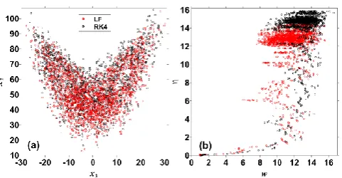
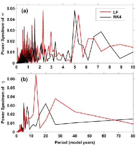
co-incident in the first 5 TUs and separate gradually then to fol-low different paths, which indicates that the difference origi-nating in these two time-differencing schemes can generate a dramatic effect due to the strong nonlinear nature of the cli-mate system. Due to the different time-differencing schemes and the coupling, the low-frequency signals are also affected significantly (seewin Fig. 1b andηin Fig. 1c, respectively). Especially the mean value ofηderived from the RK4 time-differencing scheme (the black line in Fig. 1c) is larger than that derived from the LF time-differencing scheme (the red line in Fig. 1c) after a sufficient spin-up of η. Therefore, for the high-frequency signal such as the strong nonlinear atmosphere, the different time-differencing schemes can re-sult in a difference in phase, while for a low-frequency sig-nal such as the deep ocean, the different time-differencing schemes can result in a difference not only in phase, but also in amplitude. The plots in Fig. 2 also reveal the same fact, in which the variation ofx2in the space ofx3(Fig. 2a) and the variation ofηin the space ofw(Fig. 2b) are shown for those derived from both the LF (red circle) and the RK4 (black circle) time-differencing schemes. We can see from Fig. 2a that both projections on the x2–x3 plane from the two schemes lie in the similar equilibrated positions with two attractor lobs even though they are not coincident with each other in details. However, projections on theη–wplane from the two time-differencing schemes have different posi-tions after reaching equilibrium (Fig. 2b). Figure 3 shows the power spectra ofw (Fig. 3a) andη (Fig. 3b) based on the model results between 103and 104TUs derived from the LF differencing scheme (red line) and from the RK4
time-Fig. 1. Time series of (a)x2in the first 100 TUs, (b)win the first
103TUs, and (c)ηin 104TUs derived from both the LF (red line) and the RK4 (black line) time-differencing schemes.
Fig. 2. Variation of (a)x2in the space ofx3and (b)ηin the space of
wderived from both the LF (red circle) and the RK4 (black circle) time-differencing schemes.
Fig. 3. Power spectra of (a)wand (b)ηbased on the model data between 103and 104TUs derived from both the LF (red line) and the RK4 (black line) time-differencing schemes.
two time-differencing schemes seem different distinctly, es-pecially forη, which indicates that the variability of the upper and deep oceans is strongly influenced by the type of time-stepping scheme used to integrate the model equations. How-ever, in a state-of-the-art coupled general circulation model, it is unclear yet if different time-differencing schemes can re-sult in obviously different low-frequency variability (decadal timescale and longer), which is an interesting topic that needs to be investigated further.
The above discussions show that both the time mean and the variability of the model simulation are affected strongly by the type of time-stepping scheme used. We expect to constrain the model drift caused by biased time-differencing through the DAEPC algorithm that tunes model parameters optimally according to the observational information. Next, we will design a biased twin experiment to investigate the im-pact of parameter optimization on the mitigation of coupled model bias induced by imperfect time-differencing schemes. 2.5 Biased twin experiment setup
A biased twin experiment is designed, which assumes that the imperfect time-differencing scheme is the only source of model biases. Here we define a “truth” model in which the LF time-differencing scheme is used. Starting from the ini-tial conditions described in Sect. 2.4, after the truth model is spun up for 103TUs, a time series of true states is gener-ated over a period of 104TUs. “Observations” are produced by adding a Gaussian white noise to the true values every
5 time steps for x1,2,3 and every 20 time steps for w,
re-spectively. These observational frequencies simulate the fea-ture of the real climate observing system in which the atmo-spheric observations are available more frequently than the ocean. At the same time, these observational frequencies are considered as the assimilation frequencies that the observa-tions are assimilated into the model. To simulate the lack of deep ocean measurements in the real observing system, no observation is available forη. According to Zhang (2011a), the standard deviations of the observational errors are 2 for
x1,2,3and 0.5 forw, respectively, which are derived from a
long-time model free run.
The assimilation model uses the RK4 time-differencing scheme. A Gaussian white noise with the same standard de-viation as the observational error is added to the atmospheric variable ofx2at the end of spin-up (with the same integra-tion period as the truth model) to form the ensemble initial conditions from which the ensemble filtering data assimila-tion starts. The total data assimilaassimila-tion period is 104TUs, and parameter optimization is started after 103TUs when state estimation reaches its quasi-equilibrium.
Starting from the ensemble initial conditions created above, three assimilation experiments are conducted. First, the experiment of state estimation only (SEO) that only the model states are estimated by assimilating observations into the model. Second, SEO with perturbed parameters, denoted as SEO_PP, is performed, namely, the 9 parameters (σ,κ,b,
c1,c2,c3,c4,c5, andc6) are perturbed at the same time when the ensemble initial conditions are formed by adding a Gaus-sian white noise with the standard deviation being 5 % of the default values. Third, parameter estimation is performed to optimize all these 9 parameters using the DAEPC algorithm, denoted as PP_PO. It should be noted that the other 6 pa-rameters (Om,Od,Sm,Ss,Spd, and0) act as the part of the
dynamic core that determines the timescale and period of the outer forcing of this coupled system. Therefore, they will not alter once they are determined using the default values in this study. In addition, a control run without any observational constraint, called CTRL, serves as a reference for the evalu-ation of the assimilevalu-ation results.
3 Impact of parameter optimization on climate estimation
Figure 4 shows the time series of root mean square errors (RMSEs) ofx2 in the last 100 TUs (Fig. 4a),w in the last 103TUs (Fig. 4b), andηin 104TUs (Fig. 4c) obtained from CTRL (pink line), SEO (black line), SEO_PP (red line), and PP_PO (blue line). Here, all the RMSE time series are com-puted from the difference between the ensemble mean of the model run and the truth at each time integral step over a 1-TU time window. From the black line in Fig. 4a, we can see that the estimate ofx2 in SEO does not show
Fig. 4. Time series of RMSEs of (a)x2in the last 100 TUs, (b)w
in the last 103TUs, and (c)ηin 104TUs in CTRL (pink line), SEO (black line), SEO_PP (red line), and PP_PO (blue line). Small pan-els in (a) and (b) show the detailed evolutions of RMSEs ofx2and
win SEO_PP (red line) and PP_PO (blue line) through enlarging the scale of the vertical coordinate.
Meanwhile, SEO has little contribution to the estimate of the slow-varying variables such asw or η(black line vs. pink line in Fig. 4b and c). The time mean RMSEs ofx2,w, and
ηduring the entire data assimilation period in SEO are ac-tually reduced, with respect to CTRL, by 2, 9, and 12 %, re-spectively. The improvements are not much and can hardly be observed in the time series of RMSEs. This means that within the framework of the specific dynamical core biased twin experiment setting with this simple model, the dynam-ical core misfitting of the assimilation model with respect to the truth model can function as a significant obstacle for the traditional SEO. In what follows, we will see the signif-icant improvement with parameter optimization on assimi-lation quality, which addresses the potential role of param-eter optimization in the mitigation of dynamical core model bias. Compared with SEO, estimates of all three variables (x2,w, andη) in SEO_PP demonstrate significant
improve-ment (red lines in Fig. 4a, b, and c), evidenced by one-order RMSE magnitude reduction with a small oscillation. This suggests that the perturbed physical parameters can improve the quality of state estimation greatly, since the perturba-tion of parameters can increase the spread of model states so as to increase the representation of model ensemble for the model uncertainty. The RMSE ofx2in PP_PO is reduced
with the same magnitude as in SEO_PP (blue line vs. red line in the small panel in Fig. 4a). That is to say, the im-provement in state estimation via parameter optimization is similar to that via the initial perturbation of parameters for the high-frequency atmospheric variables. However, this is not the case for the low-frequency oceanic states. The RMSE ofwin PP_PO (blue line in the small panel in Fig. 4b) is re-duced by about 66 % compared to that in SEO_PP (red line). So, the RMSE is further reduced by observation-optimized model parameters via PP_PO relative to SEO_PP. For the deep ocean, η in PP_PO is further improved significantly from SEO_PP. From Fig. 4c, it can be seen that the blue line and the red line overlap completely before 103TUs during the early state estimation only period. When the process of parameter optimization starts after 103TUs, the RMSE ofη
in PP_PO decreases from about 0.68 to about 0.2, while the RMSE in SEO_PP remains at a level of 0.68. This means that observational information can be effectively extracted by the process of parameter optimization for both the upper ocean and the deep ocean.
Figure 5 shows the time series of the ensemble means of
κ (Fig. 5a) andc2(Fig. 5b) between 900 and 1200 TUs in PP_PO. We can see that the ensemble means of the param-eters remain at their default values before 103TUs in which parameter optimization is not activated yet, but oscillate af-ter 103TUs to compensate for the bias of state estimation induced by the biased time-differencing through the back-ground error covariance between parameters and observa-tions. The oscillation frequency of κ (see Fig. 5a) in the atmospheric control equation is higher than that of c2 (see
Fig. 5b) in the oceanic equation, showing that the oscillation frequencies of parameters are affected strongly by the fre-quencies of state variables. As noted above, model parame-ters do not have any dynamically supported internal variabil-ity, and their variation depends completely on the variation of the state-parameter covariance.
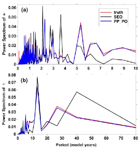
Figure 6 shows the power spectra of w (Fig. 6a) and η
Fig. 5. Time series of ensemble means of (a)κand (b)c2between
900 and 1200 TUs in PP_PO.
4 Impact of parameter estimation in different media on model bias mitigation
In this section, we investigate the impact of different me-dia parameter estimations on model bias mitigation. A series of assimilation experiments, named Case1, Case2, Case3 till Case11, as listed in Table 1, is designed to accomplish this objective.
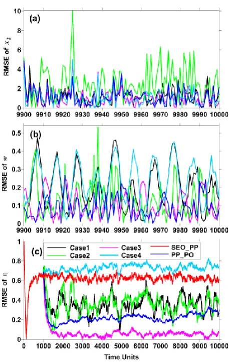
Figure 7 presents the time series of RMSEs ofx2in the last
100 TUs (Fig. 7a),win the last 100 TUs (Fig. 7b), andηin 104TUs (Fig. 7c) in Case1 (black line), Case2 (green line), Case3 (pink line), and Case4 (cyan line), respectively. Forx2
in the transient atmosphere, Case2 is the worst (green line in Fig. 7a) among all the four cases presented. The reason is thatc1andc2being optimized in Case2 are the coupling
parameters between the atmosphere variablex2and the up-per ocean variablew. Compared with the other three cases, optimizing these two coupling parameters alone cannot effi-ciently enhance the signal-to-noise ratio of the background error covariance between the parameter and the model state. For the upper ocean, it is noticed from Fig. 7b that the RM-SEs ofw in both Case1 and Case4 remain similarly larger values than the other two cases. This can be understood as follows. Case1 optimizes parameters in the atmosphere (σ,
κ, andb) and Case4 optimizes parameters in the deep ocean (c5 andc6), respectively. Neither one has a direct effect on
the upper ocean variablew, and therefore neither one is able to affectwsignificantly.
Forη, the deep ocean component, compared to SEO_PP (red line in Fig. 7c), although the RMSEs can be reduced
Fig. 6. Power spectra of (a)wand (b)ηderived from the truth (red line), SEO (black line), and PP_PO (blue line), respectively.
Table 1. Assimilation experiments list in Sect. 4.
Assimilation Optimized Ensemble Observations
experiment parameters size ofη
Case1 σ,κ,b 20 No
Case2 c1,c2 20 No
Case3 c3,c4 20 No
Case4 c5,c6 20 No
Case5 c3,c4,c5,c6 20 No
Case6 All butc5,c6 20 No
Case7 SEO_PP 200 No
Case8 PP_PO 200 No
Case9 c5,c6 200 No
Case10 SEO_PP 20 Yes
Case11 c5,c6 20 Yes
in Case1 (black line in Fig. 7c) and Case2 (green line in Fig. 7c) to some degrees, both of which remain unstable with a large oscillation. That is because observational information is used only to adjust the parameters pertinent to the high-frequency atmospheric variables instead of adjusting those pertinent to the low-frequency oceanic variables. In con-trast, Case3 has the best estimate ofη(pink line in Fig. 7c), with an RMSE reduction over 75 % compared to the case in which all parameters are optimized in PP_PO (blue line in Fig. 7c). This means that some parameters being optimized introduce noises under given conditions. Case3 optimizesc3
andc4, which represent the linear and the nonlinear
Fig. 7. Time series of RMSEs of (a)x2in the last 100 TUs, (b)win
the last 100 TUs, and (c)ηin 104TUs in Case1 (black line), Case2 (green line), Case3 (pink line), and Case4 (cyan line), respectively. The setups of the four experiments are described in Table 1. Note that the time series of RMSEs in SEO_PP (red line; only in c) and PP_PO (blue line) are also plotted as references.
estimation ofw andη significantly through the parameter optimization and the coupling between the upper ocean and pycnocline depth. It is noticed that the performance of Case4 (cyan line in Fig. 7c) is the worst among all four cases, which has an even larger RMSE than SEO_PP (red line in Fig. 7c). Parameters c5 andc6 being optimized in Case4 are in the
ηequation. Due to the absence of the observation of η,c5
andc6are estimated only indirectly through the observation of w. This suggests that only optimizing parameters perti-nent to the deep ocean compoperti-nent may lead to the noise-dominating background error covariance when other param-eters retain their default values. To explore this issue further, we performed two additional experiments, Case5 and Case6 (Table 1). Case5 optimizesc5andc6together withc3andc4.
Case6 optimizes all parameters but excludingc5andc6. It is
already learned from the discussions before that the case with
Fig. 8. Time series of RMSEs ofηin 104TUs in Case5 (green line) and Case6 (black line). The setups of the two experiments are de-scribed in Table 1. Note that the time series of RMSEs of η in SEO_PP (red line), PP_PO (blue line), and Case3 (pink line) are also plotted as references.
onlyc3andc4being optimized (i.e., Case3) has the best
per-formance. However, the additional inclusion ofc5andc6in
Case5 deteriorates the results ofη(see green line in Fig. 8), yielding larger RMSEs than the case in which all parameters are optimized in PP_PO (blue line in Fig. 8). In contrast, the RMSEs ofη in Case6 (black line in Fig. 8) have a similar mitigation to that in Case3, indicating that the exclusion of
c5andc6increases the signal-to-noise ratio during parame-ter optimization.
The poor performance of additional optimization ofc5and
c6may be associated with the insufficient ensemble represen-tation and the lack of theηobservation. To verify the first rea-son, we increase the ensemble size of SEO_PP, PP_PO, and Case4 to 200, and denote them as Case7, Case8, and Case9 (see Table 1). The time-averaged RMSE ofηin Case7 is re-duced by more than 30 % from SEO_PP, which can be seen from the green and red lines in Fig. 9. This means that the ca-pability of ensemble spread is enhanced with a large ensem-ble size. However, the RMSEs ofηin Case8 are not smaller than ones in PP_PO (black line vs. blue line in Fig. 9), which indicates that increasing the ensemble size does not improve theηestimate due to the existence of noises during signal-enhanced parameter optimization, even if the ensemble rep-resentation can be improved by increasing the ensemble size. The RMSEs ofη in Case9 are slightly larger than those in Case7 (cyan line vs. green line in Fig. 9). Thus, the noises induced by optimizing c5 and c6 cannot be removed suc-cessfully through increasing the ensemble size. However, it is clear that the performance of Case4 is indeed improved greatly when the ensemble representation is enhanced in Case9 (comparing both cyan lines in Figs. 7c and 9).
Fig. 9. Time series of RMSEs ofηin 104TUs in Case7 (green line), Case8 (black line), and Case9 (cyan line). The setups of the three experiments are described in Table 1. Note that the time series of RMSEs ofηin SEO_PP (red line) and PP_PO (blue line) are also plotted as references.
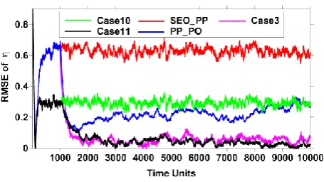
Fig. 10. Time series of RMSEs ofηin 104TUs in Case10 (green line) and Case11 (black line). The setups of the two experiments are described in Table 1. Note that the time series of RMSEs ofη
in SEO_PP (red line), PP_PO (blue line), and Case3 (pink line) are also plotted as references.
of ηin Case10 (green line in Fig. 10) are reduced signifi-cantly, but still a little larger than those in PP_PO (blue line in Fig. 10). This suggests that the signal-enhanced param-eter optimization can improve theη estimation even in the absence of observations of the deep ocean. The benefit of assimilating deep ocean observations is significant whenc5
andc6are optimized (Case11). The RMSEs ofηin Case11 (black line in Fig. 10) remain well consistent with those in Case3, indicating that the deep ocean observations may be indispensable when parameters pertinent to low-frequency components are optimized through signal-enhanced param-eter estimation. Otherwise, noises of the background error covariance will be enlarged to deteriorate the quality of cli-mate estimation, especially for the low-frequency signals.
5 Summary and discussions
A biased twin experiment framework is designed to study the mitigation of coupled model bias induced by imper-fect time-differencing through parameter optimization. In
this framework, the assimilation model includes a “biased” time-differencing scheme from the truth model that is used to produce “observations”. The leap-frog time-differencing scheme with a Robert–Asselin time filter serves as the truth run from which “observations” are drawn. The fourth-order Runge–Kutta time-differencing scheme is used for the as-similation runs. A series of asas-similation experiments is per-formed to examine the impact of parameter optimization on climate estimation and model bias mitigation, as well as the role of different media parameter estimations. Results show that the initial perturbations of parameters can enhance the ensemble spread greatly and improve the representation of the model ensemble to the model error that consists of bi-ases arising from different differencing schemes. Further-more, parameter estimation enhances the accuracy of climate estimation, especially for low-frequency signals. In addition, in a multiple timescale coupled system, parameters pertinent to low-frequency components have more impact on climate signals.
Although the parameter optimization shows promise with the simple coupled model to mitigate the model bias arising from dynamical core misfitting, further research is required to understand the impact of such model biases in coupled general circulation models (CGCMs) on climate estimation and prediction. It should be kept in mind that the concept model used in this study contains a rather large set of pa-rameters compared to the dimension of the model attractor. This will not be the case for the state-of-the-art CGCMs in general. There might also not be enough data to con-strain both the model states and additional parameters un-der the moun-dern atmospheric and oceanic observing networks. Thus potential benefits of parameter estimation vs stochastic physics, achieved in this study, need to be investigated fur-ther in the realistic scenario. Nevertheless, imperfect nume-rical schemes are usually used in CGCMs. Therefore, besides the development of more robust numerical schemes, how to optimize model parameters needs to be examined further to compensate for the deficiencies of the currently used nume-rical schemes.
Acknowledgements. This research is co-sponsored by the grants of the National Basic Research Program (2013CB430304) and National Natural Science Foundation (41030854, 41106005, 41306006, 41376013, and 41376015) of China. We are grate-ful to the editor and anonymous reviewers for the constructive comments and suggestions which have helped to improve the paper.
Edited by: D. Maraun
References
Anderson, J. L.: An ensemble adjustment Kalman filter for data as-similation, Mon. Weather Rev., 129, 2884–2903, 2001.
Anderson, J. L.: A local least squares framework for ensemble fil-tering, Mon. Weather Rev., 131, 634–642, 2003.
Asselin, R.: Frequency filter for time integrations, Mon. Weather Rev., 100, 487–490, 1972.
Collins, W. D., Blackman, M. L., Bonan, G. B., Hack, J. J., Hender-son, T. B., Kiehl, J. T., Large, W. G., and Mckenna, D. S.: The community climate system model version 3 (CCSM), J. Climate, 19, 2122–2143, 2006.
Delworth, T. L., Broccoli, A. J., Rosati, A., Stouffer, R. J., Balaji, V., Beesley, J. A., Cooke, W. F., Dixon, K. W., Dunne, J., Dunne, K. A., Durachta, J. W., Findell, K. L., Ginoux, P., Gnanadesikan, A., Gordon, C. T., Griffies, S. M., Gudgel, R., Harrison, M. J., Held, I. M., Hemler, R. S., Horowitz, L. W., Klein, S. A., Knut-son, T. R., Kushner, P. J., Langenhorst, A. R., Lee, H.-C., Lin, S.-J., Lu, S.-J., Malyshev, S. L., Milly, P. C. D., Ramaswamy, V., Rus-sell, J., Schwarzkopf, M. D., Shevliakova, E., Sirutis, J. J., Spel-man, M. J., Stern, W. F., Winton, M., Wittenberg, A. T., WySpel-man, B., Zeng, F., and Zhang, R.: GFDL’s CM2 global coupled cli-mate models. Part I: Formulation and simulation characteristics, J. Climate, 19, 643–674, 2006.
Gnanadesikan, A.: A simple predictive model for the structure of the oceanic pycnocline, Science, 283, 2077–2079, 1999. Kulhavy, R.: Implementation of Bayesian parameter estimation in
adaptive control and signal processing, Journal of the Royal Sta-tistical Society. Series D (The Statistician), 42, 471–482, 1993. Lorenz, E. N.: Deterministic non-periodic flow, J. Atmos. Sci., 20,
130–141, 1963.
Robert, A.: The integration of a spectral model of the atmosphere by the implicit method, in: Proc. WMO/IUGG Symp. on NWP, Tokyo, Japan, Japan Meteorological Society, 19–24, 1969. Smith, D. M., Cusack, S., Colman, A. W., Folland, C. K., Harris,
G. R., and Murphy, J. M.: Improved surface temperature predic-tion for the coming decade from a global climate model, Science, 317, 796–799, 2007.
Tao, G.: Adaptive control design and analysis, John Wiley & Sons, Inc., Hoboken, New Jersey, 640 pp., 2003.
Wu, X.-R., Zhang, S., Liu, Z., Rosati, A., Delworth, T., and Liu, Y.: Impact of geographic dependent parameter optimization on climate estimation and prediction: simulation with an inter-mediate coupled model, Mon. Weather Rev., 140, 3956–3971, doi:10.1175/MWR-D-11-00298, 2012.
Wu, X.-R., Zhang, S., Liu, Z., Rosati, A., and Delworth, T.: A study of impact of the geographic dependence of observing system on parameter estimation with an intermediate coupled model, Clim. Dynam., 40, 1789–1798, 2013.
Zhang, S.: Impact of observation-optimized model parameters on decadal predictions: simulation with a simple pycno-cline prediction model, Geophys. Res. Lett., 38, L02702, doi:10.1029/2010GL046133, 2011a.
Zhang, S.: A study of impacts of coupled model initial shocks and state-parameter optimization on climate prediction using a sim-ple pycnocline prediction model, J. Climate, doi:10.1175/JCLI-D-10-05003, 2011b.
Zhang, S. and Anderson, J. L.: Impact of spatially and temporally varying estimates of error covariance on assimilation in a simple atmospheric model, Tellus A, 55, 126–147, 2003.
Zhang, S., Harrison, M. J., Rosati, A., and Wittenberg, A.: System design and evaluation of coupled ensemble data assimilation for global oceanic climate studies, Mon. Weather Rev., 135, 3541– 3564, 2007.
Zhang, S., Liu, Z., Rosati, A., and Delworth, T.: A study of en-hancive parameter correction with coupled data assimilation for climate estimation and prediction using a simple coupled model, Tellus A, 64, 10963, doi:10.3402/tellusa.v64i0.10963, 2012. Zhang, X.-F., Zhang, S., Han, G.-J., and Liu, Z.: Correction of
bi-ased climate simulated by “bibi-ased” physics through parameter estimation in an intermediate coupled model, Clim. Dynam., in review, 2013a.