www.nonlin-processes-geophys.net/21/971/2014/ doi:10.5194/npg-21-971-2014
© Author(s) 2014. CC Attribution 3.0 License.
Representing model error in ensemble data assimilation
C. Cardinali1, N. Žagar2, G. Radnoti1, and R. Buizza1
1European Centre for Medium-Range Weather Forecasts, Reading, UK
2University of Ljubljana and Center of Excellence SPACE-SI, Ljubljana, Slovenia Correspondence to: C. Cardinali ([email protected])
Received: 8 July 2013 – Revised: 24 June 2014 – Accepted: 30 June 2014 – Published: 23 September 2014
Abstract. The paper investigates a method to represent model error in the ensemble data assimilation (EDA) sys-tem. The ECMWF operational EDA simulates the effect of both observations and model uncertainties. Observation er-rors are represented by perturbations with statistics charac-terized by the observation error covariance matrix whilst the model uncertainties are represented by stochastic perturba-tions added to the physical tendencies to simulate the ef-fect of random errors in the physical parameterizations (ST-method). In this work an alternative method (XB-method) is proposed to simulate model uncertainties by adding pertur-bations to the model background field. In this way the er-ror represented is not just restricted to model erer-ror in the usual sense but potentially extends to any form of back-ground error. The perturbations have the same correlation as the background error covariance matrix and their mag-nitude is computed from comparing the high-resolution op-erational innovation variances with the ensemble variances when the ensemble is obtained by perturbing only the obser-vations (OBS-method). The XB-method has been designed to represent the short range model error relevant for the data assimilation window. Spread diagnostic shows that the XB-method generates a larger spread than the ST-XB-method that is operationally used at ECMWF, in particular in the extrat-ropics. Three-dimensional normal-mode diagnostics indicate that XB-EDA spread projects more than the spread from the other EDAs onto the easterly inertia-gravity modes associ-ated with equatorial Kelvin waves, tropical dynamics and, in general, model error sources.
The background error statistics from the above described EDAs have been employed in the assimilation system. The assimilation system performance showed that the XB-method background error statistics increase the observation influence in the analysis process. The other EDA background error statistics, when inflated by a global factor, generate
analyses with 30–50 % smaller degree of freedom of signal. XB-EDA background error variances have not been inflated.
The presented EDAs have been used to generate the ini-tial perturbations of the ECMWF ensemble prediction sys-tem (EPS) of which the XB-EDA induces the largest EPS spread, also in the medium range, leading to a more reliable ensemble. Compared to ST-EDA, XB-EDA leads to a small improvement of the EPS ignorance skill score at day 3 and 7.
1 Introduction
Several operational NWP centres such as Météo-France, UK Met Office and Environment Canada have implemented an EDA system. Recently, Météo-France has implemented a six-member EDA where not only the observation uncer-tainties are represented but also the model unceruncer-tainties are explicitly taken into account. This is done by inflating the background field with a latitude-level varying factor in the ensemble (see Raynaud et al., 2009, 2012). Their first opera-tional EDA configuration (Berre et al., 2007) has been used in operations since July 2008. Flow-dependent background error variances for the operational 4D-Var assimilation sys-tem (Raynaud et al., 2011) were derived within a perfect model framework and the estimated variances were inflated “off-line” (i.e. after the ensemble has been completed) by us-ing a posteriori diagnostics (Desroziers and Ivanov, 2001). The inflation aims at representing model error contributions. Multiplicative inflation is in fact a simple and widely used technique to deal with unknown error sources. Because the off-line multiplicative inflation that was applied to the vari-ances was not accounted for in the background perturbation update, the recently implemented operational EDA configu-ration includes the multiplicative inflation to enlarge the am-plitude of forecast perturbations within the ensemble.
The Environment Canada ensemble system is based on a Kalman filter (Houtekamer and Mitchell, 2005; Houtekamer et al., 2005) and has been used operationally since January 2005. It provides an ensemble of initial conditions for the medium-range EPS (ensemble prediction system) and rep-resents both observations and model sources of uncertain-ties. In particular the model error component has been exten-sively investigated. Initially a simplified and reduced ampli-tude form of the Canadian 3D-Var background error covari-ance was used to perturb the ensemble of background fields (Houtekamer et al., 2005). Then, different ways to determine the covariance for the additive model error component have been investigated (Hamill and Whitaker, 2005) and model error perturbations are added to the ensemble analysis rather than to the background ensemble (Houtekamer and Mitchell, 2005) to account for the data assimilation weakness. More re-cently, each member has a different model version (Meng and Zhang, 2007; Fujita et al., 2007) to represent uncertainties in model representation of physical processes. As already said above, Houtekamer and Mitchell (2005) concluded that the addition of isotropic model error perturbations to the ensem-ble of analyses is found to have the largest impact in terms of ensemble spread.
An EDA was operationally implemented at ECMWF in June 2010 (Isaksen et al., 2010). The EDA ensemble con-sists of ten independent members of lower resolution (with respect to the high-resolution operational 4D-Var system) 4D-Var data assimilation systems with perturbed observa-tions and perturbed model tendencies. In particular, the servation uncertainties are represented by perturbing the ob-servations and the model uncertainties by adding stochastic perturbations to the model tendencies during the first 12 h
model evolution using the Stochastically Perturbed Parame-terization Tendency scheme (SPPT, see Palmer et al., 2009, for a review).
The ECMWF EDA provides a flow-dependent or daily model background error covariance matrix that is supposed to improve the high resolution analysis system by better rep-resenting the daily dynamical synoptic features (Raynaud et al., 2008, 2009, 2011; Buehner et al., 2010). Since its imple-mentation, the EDA has been used together with the singular vectors to initialize the operational EPS (Molteni et al., 1996; Buizza et al., 2007) and to improve the simulation of initial uncertainties (Buizza et al., 2008), one of the fundamental aspects of the EPS design.
In this paper, a different way of representing model error in the operational ECMWF EDA is presented and compared to the standard SPPT method. The model uncertainties are rep-resented by adding perturbations to the model background field. The magnitude of the perturbations varies with verti-cal level and with geographiverti-cal latitude. They are estimated from a comparison between the innovation variance of the high resolution 4D-Var system, i.e. the difference between observation and background at the observation location, and the ensemble data assimilation variance (variance taken over an ensemble of assimilations over a 3-week period) in which only observation uncertainties are represented. The model er-ror representation is therefore similar to the one introduced by Raynaud et al. (2012) at Météo-France that is referred to as the multiplicative perturbation method. The method de-scribed here is denoted as an additive perturbation method. The error represented is not restricted to the model error in the usual sense, i.e. the error that would be present in the forecast even if the initial condition were exact, but is related to any form of error, for example errors in the background co-variance matrix coming from the operational ECMWF EDA. The present paper studies the EDA sensitivity to the dif-ferent model error representations. The proposed method is compared to the operational one, which uses the stochasti-cally perturbed parameterization tendency scheme to simu-late model uncertainties, and to the EDA obtained by rep-resenting only observation uncertainties. A fourth EDA has also been designed to just quantify the impact of background cycling in the EDA where only observations are perturbed. Observation uncertainties are always equally represented in all EDAs examined.
2 Representation of uncertainties 2.1 The XB-EDA
An ensemble of analyses attempts to generate a representa-tive sample of possible states of a dynamical system. The samples are generated by the same assimilation system. From the optimal solution of the analysis problem,xa=f (xb,y), two input parameters can be identified: the observation vec-tory and the background vectorxb obtained from a short-range forecast, respectively. An ensemble of analyses can be generated by perturbing both input vectors. In particu-lar, the observations uncertainties can be represented by per-turbing vectory, whilst the model uncertainties (at least the short-range model error) can be represented by perturbing the model state vector xb. The perturbed analysis equation can be written as
˜
xa=f (xb+ζ,y+η) , (1a)
whereζandηare perturbations defined as
ζ=f (λ, l, x)B1/2ζ˜
η=R1/2η˜=σoη˜ (1b)
withf (λ, l, x)being a function of latitude (λ), model level (l) and model parameters (x).ζ˜ andη˜ are samples of vec-tors drawn from a multi-dimensional Gaussian distribution with zero mean and identity covariance matrix. To achieve that the final perturbations ζ andη have a covariance ma-trix specified by B and R, respectively, the square root of B and R is applied to the sequence of normally distributed vec-torsζ˜ andη˜. B and R are the estimated background and ob-servation error covariance matrices; they are therefore only approximations of the true covariance matrices. When R is diagonal (i.e. uncorrelated observation errors) a simple mul-tiplication by the observation error standard deviation σois applied (Eq. 1b). Only two sets of observations are perturbed with spatially correlated patterns. One is the atmospheric mo-tion vector (AMV) observamo-tion (Bormann et al., 2003) and the other set is the sea-surface temperature field (Vialard et al., 2005).
The magnitude of the final perturbation ζ is determined byf (λ, l, x)which is estimated by comparing the variance of the innovation vectord(over 3 weeks) with the ensemble data assimilation variance, Var(EDA) (estimated over an en-semble of assimilations over 3-week period), in the case the ensemble data assimilation is obtained by only perturbing the observations. The coefficient f (λ, l, x)is meant there-fore to compensate for the discrepancy between the back-ground error as obtained from the innovation d on the one hand, and the a priori background error covariance matrix B on the other. The innovation vector is the difference be-tween the observation vector y and the background coun-terpart of the observation computed by using the nonlinear
observation operator (H (xb)). Under the assumption of un-biasedness of the errors and de-correlation between the back-ground and observation errors, the backback-ground error vari-ance, as obtained from the innovation, is Var(d)−σo2. The scalar functionf (λ, l, x)is hence defined as
˜
f =f (λ, l, x)= s
Var(d)−σ2
o−Var(EDA) Var(d)−σ2
o
, (1c)
where σo2 is the prescribed observation error variance. If Var(d)−σo2 is less or equal to the EDA variance it is im-posed thatf (λ, l, x)=0. The perturbation amplitude mod-ulation hence varies in the interval [0,1]. The innovation variances have been computed for 10 hPa pressure layers for atmospheric measurements located between the sur-face and 50 hPa (wind observations), between sursur-face and 5 hPa (temperature observations), and surface and 300 hPa when humidity observations are considered. Three latitude bands, namely Northern Hemisphere (20◦N, 90◦N), South-ern Hemisphere (20◦S, 90◦S) and tropics (20◦S, 20◦N), and a 3-week data set have been considered. For theuandv com-ponent of the wind all conventional observations (radioson-des, pilots, synops, aircrafts and profilers), AMVs and scat-terometer observations have been used to compute the inno-vation variance. For temperature conventional (radiosondes and aircrafts) and AMSU-A observations, for humidity ra-diosondes and All-Sky (SSM/I and TMI radiances) observa-tions and, finally, for surface pressure all land and ocean sta-tions have been used. The variation off˜with latitude band, model level and for model parametersu,T, andq, is shown in Fig. 1. Figure 1a shows that for theu componentf˜
de-creases in the troposphere, when pressure inde-creases, down to zero in the tropics and down to 0.3 in the extratropics (level 1 at 0.01 hPa, identifies the top of the atmosphere). If obser-vations are unavailable to estimate the innovation variance, the modulation factor f˜ is kept constant, i.e. from model level 1–30 for wind, from model level 1–18 for tempera-ture and model level 1–55 for humidity. Similar results for the modulation factor are obtained for thev component of the wind (not shown). In the lower troposphere close to the surface the modulation factor globally increases on average up to 0.6. For temperature (Fig. 1b) its magnitude increases with the increase of pressure on average for the three latitude bands from 0.3 to 0.5, the tropical modulation factor always being the smallest.
For humidity (Fig. 1c) f˜ rapidly grows with the
atmo-spheric pressure level up to 0.8 (Southern Hemisphere) to-wards the surface. Concerning surface pressure, the correc-tion (1c) (not shown) is globally constant and around 0.4. During the cycling,f˜has been re-computed for retuning pur-poses using Eq. (1c) every 3 days and by using the past 3-day variance sample. However, the modulation factor has stabi-lized rather fast after 2 days of cycling.
0.7
0.6 0.5
0.4
0.3
0.2 0.1
0
1 7 13 19 25 31 37 43 Model level
M
odula
tion fac
tor
f˜
49 55 61 67 73 79 85 91
0.9
0.7 0.6 0.8
0.5 0.4 0.3 0.2 0.1 0
1 7 13 19 25 31 37 43 Model level
M
odula
tion fac
tor
f˜
49 55 61 67 73 79 85 91 0.8a)
b)
c)
0.7 N. Hemisphere Tropics S. Hemisphere 0.6
0.5 0.4 0.3 0.2 0.1 0
1 7 13 19 25 31 37 43 Model level
M
odula
tion fac
tor
f˜
49 55 61 67 73 79 85 91
Figure 1. Perturbation modulation factor f˜as a function of lat-itude band (North Hemisphere solid black line, Southern Hemi-sphere dotted line, and tropics solid grey line) and vertical model
levels (model level 1 is 0.01 hPa and 91 is on average∼1000 hPa)
for (a) zonal wind, (b) temperature, and (c) humidity. The modula-tion factor is estimated over a 3-week period.
computed along the trajectory starting from the perturbed background to correctly take into account the background changes (H is the non-linear model and observation oper-ator) and to produce a balanced perturbed field. Figure 2 schematically represents the realization of the described XB-EDA ensemble. From a control (unperturbed) analysis the two set of perturbations, η for the observations and ζ for the background, are respectively added at the beginning of the 4D-Var assimilation window to create 10 different initial
Member 3
y + η3
xb + ζ3
Member 3
y + η3
xb + ζ3
Control Analysis
Member 1 y + η1 xb + ζ1
Member 1 y + η1 xb + ζ1
Member 2 y + η2 xb + ζ2
Member 10 y + η10 xb + ζ10
12 hr
12 hr 12 hr
12 hr
Member 2 y + η2 xb + ζ2
Member 10 y + η10 xb + ζ10
Figure 2. Schematic diagram of the XB-EDA realization.
conditions (members). The two sets of perturbations are re-computed and added to the observations and the background field at every analysis cycle.
Theζperturbation accounts for the short-range model er-ror sources including the fraction of the analysis erer-ror that is due to the model error. Sources of error are therefore not only related to physical parameterizations but also to the dy-namics, the spatial and temporal discretization, the linearized physical process and the misspecification of the probability distribution of errors in the observations and the background model.
2.2 The other EDA
Table 1. Ensemble data assimilation configurations.
EDA Methodology Inflation
OBS Perturbation added to observations Y
OBS-OBS Perturbation added to observations; members background fields are from Control An. Y
ST Perturbation added to observations; perturbation added to physical parameter tendency Y
XB Perturbation added to observations; perturbation added to background N
to the interaction between the unresolved and the resolved scales, and aims to compensate for the over-dissipation oc-curring in numerical models. The SPPT scheme, designed to simulate random model errors due to physical parame-terizations, is still assumed to explain the largest source of model error in the EPS. The operational EDA configuration does not use the SPBS scheme but only the SPPT. In partic-ular, SPPT model uncertainty is simulated using the 1-scale version of the stochastically perturbed parameterization dency scheme, which perturbs the total parameterized ten-dency of physical processes. Since the 1-scale version use a timescale of 6 h, there is no need to cycle the model error perturbation across different data assimilation cycles. In the 1-scale version of the SPPT, the perturbations to the physical tendencies are defined to have a spatial correlation length of 500 km and a time correlation of 6 h, as in the original SPPT scheme (Buizza et al., 1999).
Because of the presumed ensemble analysis underdisper-sivity (to be confirmed later) a global inflation factor (=1.4) has been applied to the background error standard deviation in the OBS, OBS-OBS and ST-EDAs methods to increase the ensemble spread and to penalize the model background fur-ther with respect to the observations in the assimilation pro-cess. The static background covariance matrix has, in fact, always been inflated in the ECMWF 4DVar assimilation sys-tem to avoid the excessive weight given to the background with respect to the observations. Indeed, studies on the ob-servational influence in the analysis system have shown that globally and for a given assimilation cycle only 15 % of the information was provided by the observations while the remaining 85 % were due to the background (Cardinali et al., 2004; Cardinali, 2013). Unfortunately, the inflation is a constant that does not vary with respect to the parameters, with respect to the geographical location or weather situation and the resulting ensemble spread is simply globally ampli-fied.
3 Results
In this section EDAs with different model error represen-tations are compared and diagnosed. Each EDA includes 10 perturbed and 1 unperturbed 12 h 4D-Var assimilations (Rabier et al., 2000; Janisková et al., 2002; Tompkins and Janisková, 2004; Lopez and Moreau, 2005) at the resolution of TL399L91 (spectral triangular truncation with 399 wave
numbers and linear grid, and on 91 vertical levels) for the model forecast andTL159L91 for the minimization calcula-tion, respectively.
The four EDA schemes (Table 1) have been run for the pe-riod 1 October–15 November 2008, with twice daily 12 h as-similation cycles using observations from (21:00–09:00] and (09:00–21:00] UTC.
3.1 EDA spread
In Fig. 3 the averaged spread of the four data assimilation en-sembles is compared for the zonal wind component. The av-erage spread has been computed over the period 5 October– 15 November 2008 (the first 5 days of the EDA computation have not been included in the evaluation to take into account “spin-up”) from 6 h forecasts according to the expression
Spread(EDA)=E
v u u u t
N
P
i=1
(mi− ¯m)2
N−1
, (2a)
wheremi is theith ensemble member,N=10 andm¯ is the ensemble mean. Expectation stands for averaging over lon-gitude and over the selected period.
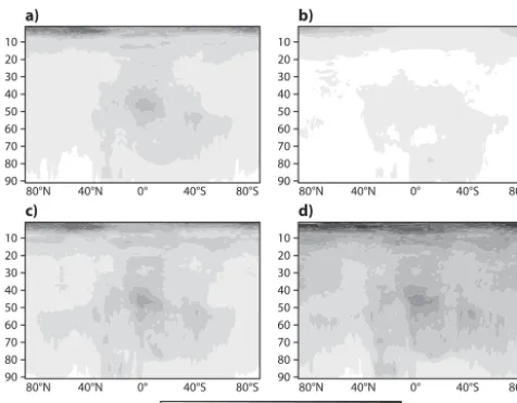
When only observation uncertainties are represented (u
wind component OBS-EDA, Fig. 3a), the spread is mainly confined to the upper stratosphere (above model level 20, i.e.
∼10 hPa) and to the troposphere (below model level 40, i.e.
0.5 1 1.5 2 2.5 3 3.5 4 5 6 7 10 0°
40°N
80°N 40°S
a) b)
c) 80°S d)
90 80 70 60 50 40 30 20 10
0° 40°N
80°N 40°S 80°S
90 80 70 60 50 40 30 20 10
0° 40°N
80°N 40°S 80°S
90 80 70 60 50 40 30 20 10
0° 40°N
80°N 40°S 80°S
90 80 70 60 50 40 30 20 10
Figure 3. Zonally averaged cross section for the period 5 October
to 15 November 2008 for the u component of the EDA spread.
(a) OBS-EDA, (b) OBS-OBS-EDA, (c) ST-EDA and (d) XB-EDA.
The vertical coordinate is model level. Contours are in m s−1.
Figure 4a shows the difference of spreads in the OBS and OBS-OBS EDAs and illustrates the impact of cycling over successive assimilation windows. Figure 4b shows the dif-ference of spreads in XB and OBS EDAs and illustrates the impact of the perturbation of the background (first part of Eq. 1b). Most of the former difference is located in the strato-sphere and in the tropics while the second extends to a large part of the troposphere, especially in the Southern Hemi-sphere. The figures also suggest that the differences are ev-erywhere positive (blank areas are values between 0 and 0.5). Figure 5 shows the reduction of globally averaged spread of the OBS-, OBS-OBS- and ST-EDAs relative to the XB-EDA for each model level and theucomponent of the wind. The spread in XB-EDA is a function of the amplitude of the per-turbation applied to the background field. The spread loss with respect to the XB ensemble is decreasing with the in-crease of model level for ST- and OBS-EDA whereas it is constant for the OBS-OBS EDAs. Close to the surface (i.e. model level 91) the first two EDAs lose 20 and 40 % spread and close to the top of the atmosphere 40–50 % on average at all latitudes, respectively.
In all EDAs the largest spread is located in the stratosphere where also the largest loss with respect to XB is observed. Similar results are obtained for the temperature field but the magnitude of the spread loss is 25 % smaller (not shown). 3.2 Spread case study
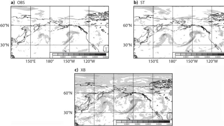
An example of spread differences among the OBS-, ST- and XB-EDAs in physical space is presented for 20–21 October 2008 in Fig. 6. In this period an intense baroclinic devel-opment took place over the northern West Pacific. In ad-dition to a mature-stage cyclone moving toward the Gulf
0.5 1 1.2 1.5 2 4
a) b)
0° 40°N
80°N 40°S 80°S
90 80 70 60 50 40 30 20 10
0° 40°N
80°N 40°S 80°S
90 80 70 60 50 40 30 20 10
Figure 4. Zonally averaged cross section from 5 October 2008 to
15 November 2008 for theucomponent of the EDA spread. (a)
Dif-ference in spreads between the OBS-EDA and the OBS-OBS-EDA spreads, (b) difference between the XB-EDA and the OBS-EDA
spreads. Vertical coordinate is model level. Contours in m s−1.
-100 -90 -80 -70 -60 -50 -40 -30 -20 -10 0
1 7 13 19 25 31 37 43 49 55 61 67 73 79 85 91
Relative Spread Loss
ST NH ST Tropics ST SH
OBS NH OBS Tropics OBS SH
OBS-OBS NH OBS-OBS Tropics OBS-OBS SH
Figure 5. Zonal wind field relative average spread loss of OBS, ST, OBS-OBS EDA with respect to XB EDA at every model level and for Northern (dashed line) and Southern (solid line) Hemisphere and tropics (dotted line).
of Alaska, a deep cyclogenesis took place about 4000 km westward at about 50◦N, 180◦W (not shown). All methods
0
a) OBS b) ST
c) XB
0.0001 180° 150°E 30°N
60°N
150°W 120°W 150°E 180°
30°N 60°N
150°W 120°W
180° 150°E 30°N
60°N
150°W 120°W
0.0002 0.0003 0.0004 0.0005 0 0.0001 0.0002 0.0003 0.0004 0.0005
0 0.0001 0.0002 0.0003 0.0004 0.0005
Figure 6. 6 h forecast of vorticity field spread at 850 hPa valid on 21 October 2008 at 12:00 UTC. (a) OBS-EDA, (b) ST-EDA and (c) XB-EDA.
3.3 Modal diagnosis of the ensemble spread
The discussion of the results in the previous sections is complemented hereafter with the diagnosis of the ensem-ble spread in terms of normal modes as described in Žagar et al. (2011). The 10 members of the four ensemble experi-ments are projected onto a set of three-dimensionally orthog-onal vectors which are eigensolutions of the Navier–Stokes equations linearized about an horizontally homogeneous sta-ble state of rest. This projection allows the attribution of the ensemble spread according to various horizontal and vertical scales as well as linearly balanced (quasi-geostrophic) and unbalanced (inertio-gravity, IG) parts of the flow. In Žagar et al. (2011), the method was applied to the analysis of the ensemble spread of the DART-CAM system whereas Žagar et al. (2013) used the method to study the balance proper-ties of the ECMWF EDA system. In the ECMWF EDA for July 2007, it was found that about 50 % of the short-range forecast-error variance was associated with the IG modes and that the eastward-propagating IG component was dominant on all scales. Both results were associated with the majority of EDA variance being present in the tropics. On the other hand, the ensemble spread of the DART-CAM ensemble was characterized by a prevalence of the westward-moving IG modes which was found to be related to the covariance in-flation. These studies suggest that the normal mode function (NMF) expansion is a useful diagnostic of EDA systems.
In the present study, we followed Žagar et al. (2013) to analyse model levels under 10 hPa (model levels 19–91, to-talling 73 levels) in order to avoid very large spread in the mesosphere (see Fig. 3) that projects strongly on the leading vertical modes and can obscure the interpretation
of the results. For the presented diagnostics, 6 h forecast starting at 18:00 UTC in the period 18 October–16 Novem-ber 2008 are used (30 samples) for 10 ensemble mem-bers. The analysed data on the N64 Gaussian grid are pro-jected onto 85 zonal wave numbers, 50 vertical modes and 40 meridional modes for each motion type, namely balanced, eastward gravity (EIG mode) and westward inertio-gravity (WIG mode).
In modal space, the ensemble spread based onNensemble members is defined as
Sν=
"
1
N−1 N
X
i=1
gHν
χυ,i−χυ
·χυ,i−χυ
∗ #1/2
, (2b)
whereχν,i is a non-dimensional complex projection coeffi-cient for an ensemble member i while ν is a four-indices modal index which contains information about the zonal wave number, the meridional mode, the vertical mode and the wave type. The overbar stands for averaging overN ensem-ble members, i.e.χυ is the ensemble mean,χυ=N1
N
P
i=1
b) ST
102
2
1 3 4 6 8
Zonal wavenumber
Spr
ead (ms
–1)
1115 25 40 70 101
d) OBS-OBS
102
2
1 3 4 6 8
Zonal wavenumber
Spr
ead (ms
–1)
1115 25 40 70 101
ROT EIG WIG a) XB
102
2
1 3 4 6 8
Zonal wavenumber
Spr
ead (ms
–1)
1115 25 40 70 101
c) OBS
102
2
1 3 4 6 8
Zonal wavenumber
Spr
ead (ms
–1)
1115 25 40 70 101
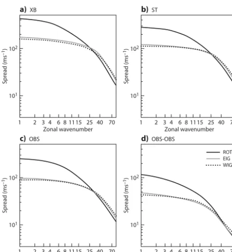
Figure 7. Time-averaged ensemble spread in the balanced and inertio-gravity modes for (a) XB-EDA, (b) ST-EDA, (c) OBS- and (d) OBS-OBS EDA. Black curves correspond to the spread associ-ated with balanced modes (ROT), grey curves to spread due to east-erly propagating inertia-gravity (EIG) modes whereas dotted curves represent spread due to westerly propagating inertia-gravity modes (WIG).
Spectra of the balanced, EIG and WIG energy spread as a function of the zonal wave number are shown in Fig. 7. In agreement with what has been presented so far, the ensemble spread in the XB-EDA dominates over the ST-EDA and OBS-EDA at all scales and for all three motion types. The ST-OBS-EDA spread is closer to the OBS-EDA spread than to the XB-EDA spread. In all experiments, the EIG spread dominates over WIG at largest horizontal scales and in XB-EDA it is greater than the WIG spread on all scales due to the equatorial Kelvin modes (not shown). The XB-, ST- and OBS-EDAs have a smaller percentage of their spread in the largest scale with re-spect to OBS-OBS-EDA. Below zonal wave number 10, there is around 30 % of the total spread for all experiments, vary-ing from 28 % for ST-EDA to 34 % for OBS-OBS-EDA (not shown).
On average, the total spread in XB-EDA is between 1.7 and 1.6 times greater than the OBS-EDA spread. The ST-EDA spread is around 1.25 times of the OBS-ST-EDA spread. Both XB- and ST-EDA add relatively more spread in the IG part than in the balanced part with respect to OBS-EDA. Instead, the experiment without cycling (OBS-OBS-EDA) counts only for 40 % of the spread of OBS-EDA for all modes (not shown).
b) ST 70 65 60 55 50 45 40 35 30 25 20 2
1 3 4 6 8
Zonal wavenumber
% of the t
otal spr
ead
1115 25 40 70
70 65 60 55 50 45 40 35 30 25 20 2
1 3 4 6 8
Zonal wavenumber
% of the t
otal spr
ead
1115 25 40 70 70 65 60 55 50 45 40 35 30 25 20 2
1 3 4 6 8
Zonal wavenumber
% of the t
otal spr
ead
1115 25 40 70
70 65 60 55 50 45 40 35 30 25 20 2
1 3 4 6 8
Zonal wavenumber
% of the t
otal spr
ead
1115 25 40 70
d) OBS-OBS
ROT EIG WIG IG a) XB
c) OBS
Figure 8. Ratios of the balanced (ROT), EIG, WIG and IG (EIG + WIG) spread to the total spread in each zonal wave num-ber for (a) XB-EDA, (b) ST-EDA, (c) OBS-EDA and (d) OBS-OBS-EDA. The ratios are multiplied by 100. Black curves correspond to balanced modes (ROT), grey to easterly propagating inertia-gravity modes (EIG), dotted to westerly propagating inertia-inertia-gravity (WIG) while dashed curves correspond to all inertia-gravity modes (IG = EIG + WIG).
When the spread is summed up across all scales, the per-centages of ROT, EIG and WIG spread in the four experi-ments are 43, 28, 29 % for OBS-OBS-EDA, 41, 29, 30 % for OBS-EDA, 39, 30, 31 % for ST-EDA, and 40, 31, 29 % for XB-EDA, respectively. Overall, the XB-EDA is the only ex-periment with total EIG spread greater than the WIG spread. As can be seen in Fig. 8, which presents ratios between the balanced, EIG and WIG spread with the total spread as a function of the zonal scale, this applies for every zonal wave number. The dominance of the EIG spread in the XB-EDA is most likely associated with the larger tropical spread in this experiment (see also Fig. 3) and it is also in agreement with Žagar et al. (2013), who presented the same conclusion for the 3 and 12 h forecast-error variances in an earlier model cy-cle. As discussed there, easterly propagating tropical modes represent the most important variability and largest forecast error source in the tropics.
while ST-EDA increases more the WIG spread than the EIG spread with respect to OBS-EDA (not shown). This result may be a consequence of the variance inflation as found in Žagar et al. (2011) for an ensemble Kalman filter system DART/CAM.
Figure 8 also shows that in all experiments the IG spread is dominant over the balanced spread for the zonal wave num-bers greater than 10. At the shortest analysed scales, the IG spread makes about 70 % of the total spread. Although dif-ferences in the EIG and WIG spread may seem small when expressed in percentages, they illustrate a sensitive balance affected either dynamically (larger growth of forecast errors in tropical easterly modes) or artificially (variance inflation) with potentially major impacts on subsequent forecasts. 3.4 Using EDAs to define background error covariance
matrices for assimilation
Background error statistics, the static B covariance matrix, computed from the OBS-, ST- and XB-EDAs are provided to the assimilation system and three TL399L91TL255 res-olution analyses are computed for the period 5 October– 15 November 2008. Because at the time these experiments were performed, the operational configuration was still us-ing the static B matrix, the use of a “flow dependent” B ma-trix was not possible. Description of the computation of the static B matrix from an ensemble analysis can be found in Fisher (2003); see also Derber and Bouttier, 1999, for co-variance modelling. The background error coco-variance ma-trix is modelled using coordinate transformations and spher-ical wavelet techniques (Fisher, 2003). In addition, a non-linear, analytical balance is included in the covariance model (Fisher, 2003). The OBS, ST and XB analyses use, respec-tively, OBS-, ST- and XB-EDAs estimated B matrices. Diag-nostics have been performed to assess the background error covariance impact on the assimilation system. The analysis experiments have the same name of the EDA experiments but bold fonts are used instead.
The first diagnostic presented is based on the observation influence (OI) (Cardinali et al., 2004; Cardinali, 2013) which quantifies the observational leverage in the analysis. The mean OI is the degree of freedom for signal, DFS, or total observation influence (Tukey, 1972; Velleman and Welsch, 1981; Wahba et al., 1995; Purser and Huang, 1993) divided by the total number of observationN:
OI=DFS
N =
tr(HTLK)T
N . (2c)
HTL is the linear observation operator and K is the gain matrix. OI and DFS depend on the assigned accuracy of the observations and background as well as the model itself which is a space and time propagator. The DFS quantifies the number of statistically independent directions constrained by each observation. Differences in the OI or DFS in the three assimilation experiments reflect differences in the B
matri-0 0.1 0.2 0.3 0.4 0.5 0.6 0.7 0.8 0.9
AMSU-A AIRS IASI
GPS-RO AMSU-B HIRS SSMI OZONE SCAT Vertical Profiler
AMV
OI
OBS ST XB
Figure 9. Global average observation influence (OI) for the differ-ent observation types assimilated in the XB (black line), ST (dark grey line), OBS (light grey line) 4DVar analyses. AMSU-A and AMSU-B are microwave radiances, AIRS and IASI and HIRS in-frared radiances, SSMI microwave imager radiance, GPS-RO satel-lite GPS radio occultation, OZONE retrieval, SCAT retrieved wind information from microwave scatterometer, atmospheric motion vector (AMV) from geostationary cloud imagery and vertical filer consists of wind from radiosonde, pilot, aircraft and wind pro-filer observations.
ces. The OI is proved to be bounded between 0 and 1; 0 in-fluence indicates that an observation has not had inin-fluence on the estimate but only the background counted whilst OI = 1 means that an entire degree of freedom has been devoted to fit that observation point. The OI can be gathered e.g. by ob-servation type; in Fig. 9 the OI in OBS, ST and XB analyses is shown for different satellite and conventional observation types. Results indicate that XB shows the largest OI.
In particular, the largest OI increase is noticed for wind reporting observations (0.3 OBS, 0.5 ST and 0.7 XB), GPS-RO (0.2 OBS, 0.3 ST and 0.7 XB), AMSU-B radiances (0.2 OBS, 0.3 ST and 0.4 XB) and All-Sky SSMI radiances (0.1 OBS, 0.2 ST and 0.3 XB). The OI diagnostic indicates that when model errors are under-represented in the ensem-ble analysis, the background error statistics are also under-estimated and the observations have smaller leverage in the assimilation procedure. XB analysis provides better observa-tions fit (not shown) in agreement with the higher OI. XB DFS is 50 % larger than OBS and 30 % larger than ST DFS. A measure of the consistency of the assimilation sys-tem is provided by the diagnostics on the background-error statistics computed in observation space (Talagrand, 2002; Desroziers et al., 2005). If the K gain matrix is consistent with the “true” covariances for background and observation errors, the innovationdand the analysis errors should be de-correlated from a statistical point of view. It can be simply shown (Desroziers et al., 2005) that the covariance between the analysis increment in observation space (Hxa−Hxb) and the innovation vector (d), quantities archived during the as-similation procedure, should satisfy
HTLBHTTL≈E
h
(HTLxa−HTLxb)dT
i
The assigned background error variances,HTLBHTTL(in ob-servation space), are also archived; therefore the difference between the assigned and estimated background variances can be computed and averaged over the period of interest. In the context of linear estimation theory, a consistent unbiased analysis should result in no difference between the estimated and assigned background error variance. The following vari-ance consistency check (VCC):
VCC=
HTLBHTTL
estimated− HTLBH T TL
assigned
HTLBHTTL
estimated
(2e)
measures the difference between the background error vari-ances estimated from the analysis residuals (Desroziers et al., 2005) and the background error variances assigned from the ensemble analysis normalized with respect to the esti-mated ones.
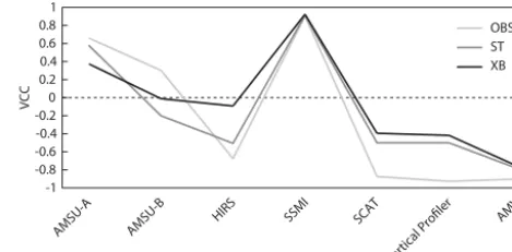
The VCC computed for the period 5 October–15 Novem-ber 2008 for OBS, ST and XB analyses shows small but non-zero values. Figure 10 shows the VCC for AMSU-A and AMSU-B, HIRS, SSMI, SCAT, vertical profilers and AMV: XB VCC is smaller than OBS and smaller than or similar to ST.
3.5 EDA-only based ensemble prediction system (EPS) forecasts
Buizza et al. (2008) proposed to use EDA-based perturba-tions in the ECMWF operational ensemble prediction system (EPS), and in June 2010 EDA-based perturbations have been introduced in the EPS to improve the simulation of initial uncertainties (Isaksen et al., 2010). The replacement in the EPS of the evolved singular vectors with EDA-based pertur-bations improved substantially the EPS spread over the trop-ics, with a detectable impact in the early forecast range also over the extratropics. A positive impact was also detected on the EPS skill.
The three EDAs discussed in this work can be used to as-sess the sensitivity of EPS forecasts to the EDA configura-tions. Two types of ensembles were run: the first type cluded EDA-only perturbations, and the second type also in-cluded singular vectors (this is the configuration of the oper-ational EPS). Since the impact of the EDA is more evident in the EDA-only type, attention will be focused mainly on them. EDA-only EPSs have been run with the perturbations defined using the OBS-, ST and XB-EDAs. All three EPS configu-rations included 50 perturbed and 1 unperturbed members, with variable resolution TL399L62 between forecast day 0 and 10, and TL255L62 between forecast day 10 and 15 (in uncoupled mode). All forecasts have been run with both the SPPT and the SPBS stochastic scheme as in the operational EPS (in other words, even the OBS-EPS that starts from the OBS-EDA-based perturbations that did not use any stochas-tic model, included stochasstochas-tic perturbations in each of the 50 perturbed members). Forecasts have been run for 18 cases,
-1 -0.8 -0.6 -0.4 -0.2 0 0.2 0.4 0.6 0.8 1
AMSU-A AMSU-B HIRS SSMI SCAT
Vertical Profiler AMV
VCC
OBS ST XB
Figure 10. VCC for AMSU-A and AMSU-B, HIRS, SSMI, SCAT, vertical profilers and AMV from XB (black line), ST (dark grey line), OBS (light grey line) analyses.
with initial conditions from 12 October to 14 November 2008 every other day (with 12:00 UTC as initial time).
In all ensemble configurations, following the methodology used in the ECMWF EPS operational at the time when the experiments were conducted (for more details, see Isaksen et al. (2010) and references therein), the EDA-based compo-nent of the 50 EPS initial perturbations have been constructed by (a) defining 10 EDA-based perturbations by computing the difference between each of the 10 EDA perturbed mem-bers and the unperturbed (control) member and by (b) adding and subtracting these EDA-based perturbations from the un-perturbed analysis, defined by the ECMWF operational high-resolution 4D-Var system. Since this procedure provides only 20 perturbations, EPS members 21–40 have the same initial EDA-based perturbations as members 1–20, and EPS mem-bers 41–50 have the same as memmem-bers 1–10. The fact that up to three EPS members can use the same EDA-based per-turbations is not a problem in the ensembles run with initial perturbations generated using both EDA-based perturbations and singular vectors (as is the case for the operational EPS), since 25 different SV-based initial perturbations are also used to generate the 50 positive and negative SV-based perturba-tions. For the EDA-only ensembles, the EPS members start-ing with the same EDA-based perturbation diverge, albeit in a slower way than the ensembles initialized by blending EDA- and SV-based perturbations, since each EPS member is integrated with different model error perturbations gener-ated by the stochastic physic schemes.
C. Cardinali et al.: Representing model error in ensemble data assimilation 981 0 1 2 3 4 5 6 0 1 2 3 4 5 6 RMS
a) Northern Extra-tropics
OBS 850hPa
c) Tropics
850hPa
850hPa
ST XB
RMS
b) Southern Extra-tropics
fc-step (d)8 6 4 2
0 10 12 14
fc-step (d)8 6 4 2
0 10 12 14
fc-step (d)8 6 4 2
0 10 12 14
0 1 2 3 RMS 0 1 2 3 4 5 6 0 1 2 3 4 5 6 RMS
a) Northern Extra-tropics
OBS 850hPa
c) Tropics
850hPa
850hPa
ST XB
RMS
b) Southern Extra-tropics
fc-step (d)8 6 4 2
0 10 12 14
fc-step (d)8 6 4 2
0 10 12 14
fc-step (d)8 6 4 2
0 10 12 14
0 1 2 3 RMS 0 1 2 3 4 5 6 0 1 2 3 4 5 6 RMS OBS 850hPa
c) Tropics 850hPa
850hPa
ST XB
RMS
fc-step (d)8 6 4 2
0 10 12 14
fc-step (d)8 6 4 2
0 10 12 14
fc-step (d)8 6 4 2
0 10 12 14
0 1 2 3
RMS
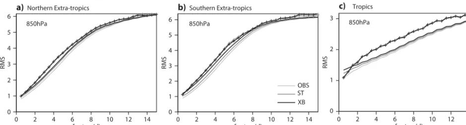
Figure 11. Averaged spread measured by the standard deviation (solid lines) and error of the ensemble mean (lines with symbols) of the EPS run with EDA-only perturbations generated from OBS-EDA (light grey), ST-EDA (dark grey) and XB-EDA (black). Results refer to
the zonal wind component at 850 hPa over the (a) Northern Hemisphere (20–80◦N), (b) Southern Hemisphere (20–80◦S) and (c) tropics
(20◦S–20◦N). The average has been computed considering 18 cases, each with 51-member EPS forecast with initial condition from 12 to
14 November 2008, every other day (12:00 UTC only).
In this work, attention has been focused on three as-pects: firstly the ensemble reliability, i.e. the consistency between forecast probabilities and observed frequencies of occurrence, measured by the agreement between ensem-ble spread and ensemensem-ble-mean error; secondly the error of the ensemble-mean forecast; and thirdly the skill of abilistic forecasts measured by the continuous rank prob-ability skill score (CRPSS) and the ignorance score. Con-sidering the first aspect, in a reliable ensemble, on average the spread of the system measured by the standard devia-tion should be equal to the average error of the ensemble mean. This property follows from the fact that in such a sys-tem, one ensemble member can be considered as the verifi-cation (Buizza et al., 2005; Palmer et al., 2006). Figure 11 shows the EPS spread (measured by the standard deviation) and the root-mean-square error of the ensemble mean fore-cast for the zonal wind at 850 hPa (verified against the opera-tional high resolution analysis), computed over the Northern Hemisphere (20–80◦N, Fig. 10a), over the Southern Hemi-sphere (20–80◦S, Fig. 10b) and over the tropics (20◦S– 20◦N, Fig. 10c).
Figure 11 shows that for all configurations the ensem-bles are underdispersive, especially over the tropics, indi-cating that EDA-only perturbations, if used as generated by the EDA and not scaled, are not sufficient to produce re-liable ensemble forecasts. Among the EDA configurations, the XB-EPS has the largest spread, with differences evident up to about forecast day 10. Considering the error of the en-semble mean, Fig. 11 shows that the enen-semble mean fore-casts are very similar, almost undistinguishable for most of the forecast times, with the XB-EPS showing the smallest er-ror for the forecast times when the spread is closer to the ensemble-mean root-mean-square error level (e.g. between forecast day 5 and 8 over the SH and between forecast day 5 and 10 over the tropics).
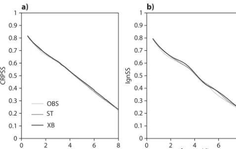
Considering the skill of probabilistic forecasts, all the met-rics mentioned above have been considered, and since results are all consistent, only CRPSS and ignorance skill scores will be shown. The CRPSS is the equivalent of the mean squared error for single forecasts, and give a measure of the average distance between the forecast and observed distribu-tions; the corresponding skill score, the CRPSSs have been computed using a climatological probabilistic forecast as ref-erence (thus a perfect probabilistic forecast would score 1, and a forecast as skillful as climatology 0). The ignorance skill score is a logarithmic score defined using informa-tion theory (Roulston and Smith, 2002), based on the infor-mation deficit (or ignorance) in the forecast. According to Benedetti (2010), for probabilistic forecast systems the ig-norance score and skill scores are more fundamental scores than the Brier score and skill scores, given that these latter are second-order approximations of the former. A clear ad-vantage of these two scores compared to the Brier score and skill score, or the area under a relative operating character-istic, is that both the CRPSS and the ignorance skill score consider the whole forecast probability distribution function of forecast states, and not simply some specific event (e.g. the probability of a variable exceeding a certain threshold). Thus, they provide a more complete assessment than these latter two (Wilks, 1995).
fc-step (d)4 2
0 6 8 0 2 4 6
0 0.1 0.2 0.3 0.4 0.5 0.6 0.7 0.8 0.9 1
CRPSS
OBS ST XB
a)
fc-step (d) 0
0.1 0.2 0.3 0.4 0.5 0.6 0.7 0.8 0.9 1
IgnSS
b)
Figure 12. Average CRPSS (a) and ignorance score (b) of EPS run with EDA-only perturbations generated from OBS-EDA (light grey), ST-EDA (dark grey) and XB-EDA (black) for temperature at 850 hPa over the Southern Hemisphere. The average has been computed considering 18 cases, 51-member EPS forecast with ini-tial condition from 12 to 14 November 2008, every other day (12:00 UTC only).
Concluding, these results based on EDA-only ensembles indicate that the use of the XB-EDA in the EPS would lead to a slightly better match between spread and error, i.e. a bet-ter reliability, and to similar forecast skill as the use of the ST- and OBS-EDAs The EPS experiments based on EDA-based perturbations and singular vector perturbation indi-cate smaller spread differences, detectable only up to fore-cast day 5 instead of day 10, and practically no differences in skill (not shown).
4 Conclusions
In this paper, the representation of model error in the ECMWF 4DVar Ensemble Data Assimilation (EDA) system by additively perturbing the background field is shown. The method follows the idea used in the Meteorological Service of Canada (MSC) ensemble Kalman filter (Houtekamer et al., 2005) and in the ARPEGE 4D-Var system (Raynaud et al., 2012) to account for model uncertainties in the EDA by perturbing the model background field. In the MSC ensem-ble Kalman filter the perturbation magnitude is globally con-stant (but the representation of other errors is also consid-ered) whilst at Météo-France the perturbation, as a function of latitude band and model level, is multiplied to the back-ground field (multiplicative approach). Here, the additive ap-proach is presented.
The idea behind it is that a large fraction of model error is represented by the short-range forecast error. Thus perturb-ing the 12 h model forecast would include error sources intro-duced by dynamics, spatial and temporal discretization and, in the case of assimilation, linearized physical processes and the misspecification of the probability distribution of errors
in the observations and the numerical background model. The proposed methodology, contrary to the stochastically perturbed parameterization tendency scheme, does not re-quire routine diagnostic and tuning.
Ensembles of data assimilation with different representa-tions of model error have been compared. In particular, two more EDAs are examined, all with the same methodology to represent the observation uncertainties but different tech-niques to account for model uncertainties. One model error representation technique is based on the assumption that ran-dom model errors due to the physical process parameteri-zations are the main model error source (ST-EDA). In the ST-EDA, stochastic perturbations are added to the physical model tendency at each model time step. The other ensem-ble considered (OBS-EDA) only includes an observation er-ror representation, which implicitly modifies the background fields in the assimilation cycling process. In the additive XB-method, the magnitude of the perturbation is calculated by comparing the variance of the innovation vector of the high resolution analysis system with the ensemble data assimila-tion variance in which the ensemble data assimilaassimila-tion is pro-duced by only perturbing the observations. The perturbation is a function of latitude band, vertical model level and the model parameter.
the only experiment which contains more spread in the east-erly propagating IG modes than in the westeast-erly IG compo-nent. It is believed that this is due to the tropical flow proper-ties which are strongly influenced by the easterly propagating Kelvin waves. Although more investigation is needed to con-firm this interpretation, the increase of spread in the westerly IG mode for the ST is likely to be related to the inflation of the model background error variances (as was found by Žagar et al., 2011, for the DART-CAM ensemble). In fact, it should be kept in mind that OBS- and ST-EDAs include a global inflation factor of the background error variances that penalizes the model background further with respect to the observations. The inflation is a spatial and temporal constant that does not depend on synoptic weather developments but only intends to introduce larger ensemble spread.
The covariance matrices produced by the three ensemble analyses have been provided to a higher resolution data as-similation system. The diagnostic performed on the three re-sulting analyses show that the largest observation influence (OI) is obtained from the assimilation system with XB-EDA background statistics. This is due to the larger background error variances. When the analysis residual diagnostic is ap-plied to investigate the consistency of the assimilation sys-tems considered, systematical smaller differences are found with XB showing closer agreement between the assigned and estimated background error variances.
Finally, the three EDAs have been used in ensemble pre-diction mode. Since June 2010, EDA-based perturbations have been used with singular vectors to simulate initial un-certainties in the ECMWF EPS (Buizza et al., 2008; Isak-sen et al., 2010). Results have indicated that the use of the XB-EDA in the EPS would lead to the largest spread, with differences evident up to about forecast day 10 and with the smallest error for forecast times from day 5 to 8 over South-ern Hemisphere and from day 5 to 10 over the tropics when the spread is closer to the ensemble mean root-mean-square error. In terms of EPS forecast skill, very small but consis-tent improvements up to day 7 have been detected when, in particular, the ignorance score is used.
In conclusion, the XB-method discussed in this work is shown to be a valuable alternative of the method used in the current ECMWF EDA to simulate model uncertainty in the ensemble analysis. It accounts for different sources of error coming from the dynamics, the parameterizations, the lin-earization and interpolation schemes and it is easier to tune and maintain. The tuning of the perturbation is performed au-tomatically every 3 days from a 3-day sample of the high res-olution operational innovations. A possible extension of the work presented would be to combine the background bation method with the stochastic physical tendency pertur-bation method or other methodologies that are considered to simulate longer range random model error sources. The es-timation of the background perturbations magnitude should, in this case, be achieved by comparing the innovations of the high resolution analysis system with the EDA in which not
only the observations are perturbed but also e.g. stochastic perturbations are added to the physical model tendency, that is, the ST-EDA.
The Supplement related to this article is available online at doi:10.5194/npg-21-971-2014-supplement.
Acknowledgements. The authors thank Elias Holm, who provided the B matrices computed from the ensemble of background states from the different EDAs considered in this study. The authors are very thankful to Gerald Desroziers and Loïk Berre for fundamental discussions on the methodology applied here. The authors are also very grateful to the thorough and constructive review provided by two reviewers, Antony Weaver and an anonymous one, which not only has improved the manuscript but has enriched our understanding of ensemble analysis methodologies.
Edited by: O. Talagrand
Reviewed by: T. Weaver and one anonymous referee
References
Benedetti, R.: Scoring rules for forecast verification, Mon. Weather Rev., 138, 203–211, 2010.
Berner, J., Shutts, G., Leutbecher, M., and Palmer, T. N.: A Spectral Stochastic Kinetic Energy Backscatter Scheme and its Impact on Flow-dependent Predictability in the ECMWF Ensemble Predic-tion System, J. Atmos. Sci., 66, 603–626, 2008.
Berre, L., Pannekoucke, O., Desroziers, G., Stefanescu, S. E., Chap-nik, B., and Raynaud, L.: A variational assimilation ensemble and the spatial filtering of its error covariances: increase of sam-ple size by local spatial averaging, ECMWF Workshop Proceed-ings on Flow Dependent Aspect of Data Assimialtion, 11–13 June 2007, 151–168, 2007.
Bormann, N., Saarinen, S., Kelly, G., and Thépaut, J.-N.: The spa-tial structure of observation errors in atmospheric motion vectors from geostationary satellite data, Mon. Weather Rev., 131, 706– 718, 2003.
Brier, G. W.: Verification of forecasts expressed in terms of proba-bility, Mon. Weather Rev., 78, 1–3, 1950.
Buehner, M., P. L. Houtekamer, C., Charette, and Mitchell, H. L.: Intercomparison of Variational Data Assimilation and Ensem-ble Kalman Filter for Global Deterministic NWP. Part II: One-Month experiments with real observations, Mon. Weather Rev., 138, 1567–1586, 2010.
Buizza, R., Miller, M., and Palmer, T. N.: Stochastic representation of model uncertainties in the ECMWF ensemble prediction sys-tem, Q. J. Roy. Meteor. Soc., 125, 2887–2908, 1999.
Buizza, R., Houtekamer, P. L., Toth, Z., Pellerin, G., Wei, M., and Zhu, Y.: A comparison of the ECMWF, MSC and NCEP Global Ensemble Prediction Systems, Mon. Weather Rev., 133, 1076– 1097, 2005.
Buizza, R., Leutbecher, M., and Isaksen, L.: Potential use of an en-semble of analyses in the ECMWF Enen-semble Prediction System, Q. J. Roy. Meteor. Soc., 134, 2051–2066, 2008.
Cardinali, C.: Observation influence diagnostic of a data assimila-tion system, in: Data Assimilaassimila-tion for Atmospheric, Oceanic and Hydrologic Applications (Vol. II), Springer Berlin Heidelberg, 89–110, 2013.
Cardinali, C., Pezzulli, S., and Andersson, E.: Influence matrix dag-nostics of a data assimilation system, Q. J. Roy. Meteor. Soc., 130, 2767–2786, 2004.
Derber, J. and Bouttier, F.: A reformulation of the background er-ror covariance in the ECMWF global data assimilation system, Tellus A, 51, 195–222, 1999.
Desroziers, G. and Ivanov, S.: Diagnosis and adaptive tuning of observation-error parameters in a variational assimilation, Q. J. Roy. Meteor. Soc., 127, 1443–1452, 2001.
Desroziers, G., Berre, L., Chapnik, B., and Poli, P.: Diagnosis of ob-servation, background and analysis error statistics in observation space, Q. J. Roy. Meteor. Soc., 131, 3385–3396, 2005.
Fisher, M.: Background error covariance modeling, in: Proceed-ings of the ECMWF Seminar on recent developments in data as-similation for atmosphere and ocean, ECMWF, 45–63, available at: http://old.ecmwf.int/publications/library/do/references/show? id=86048, 2003.
Fujita, T., Stensrud, D. J., and Dowell, D. C.: Surface data assimila-tion using an ensemble Kalman filter approach with initial con-dition and model physiss uncertainties, Mon. Weather Rev., 135, 1846–1868, 2007.
Gauthier, P., Buehner, M., and Fillion, L.: Background-error statis-tics modelling in a 3D variational data assimilation scheme: Es-timation and impact on the analyses, in: Proceedings of ECMWF workshop on Diagnosis of data assimilation systems, ECMWF, Reding UK, 131–145, 1999.
Hamill, T. M. and Whitaker, J. S.: Accounting for the error due to unresolved scales in ensemble data assimilation: a comparison of different approaches, Mon. Weather Rev., 133, 3132–3147, 2005. Houtekamer, P. L. and Mitchell, H. L.: Ensemble Kalman Filtering,
Q. J. Roy. Meteor. Soc., 131, 3269–3289, 2005.
Houtekamer, P. L., Lefaivre, L., Derome, J., Ritchie, H., and Mitchell, H. L.: A system simulation approach to ensemble pre-diction, Mon. Weather Rev., 124, 1225–1242, 1996.
Houtekamer, P. L., Pellerin, G., Buehner, M., Charron, M., Spacek, L., and Hansen, B.: Atmospheric data assimilation with an en-semble Kalman Filter: Results with real observations, Mon. Weather Rev., 133, 604–620, 2005.
Houtekamer, P. L., Mitchell, H. L., and Deng, X.: Model error representation in an Operational Ensemble Kalman Filter, Mon. Weather Rev., 137, 2126–2143, 2009.
Isaksen, L., Haseler, J., Buizza, R., and Leutbecher, M.: The new Ensemble of Data Assimilation, ECMWF, Shinfield Park, Read-ing RG2-9AX, UK, Newsletter n. 123, 17–21, 2010.
Lopez, P. and Moreau, E.: A convection scheme for data assimila-tion: Description and initial tests, Q. J. Roy. Meteor. Soc., 131, 409–436, 2005.
Janisková, M., Mahfouf, J.-F., Morcrette, J.-J., and Chevallier, F.: Linearized radiation and cloud schemes in the ECMWF model: Development and evaluation, Q. J. Roy. Meteor. Soc., 128, 1403– 1423, 2002.
Meng, Z. and Zhang, F.: Tests of an ensemble Kalman filterfor mesoscale and regional-scale data assimilation. Part II: Imperfect model experiments, Mon. Weather Rev., 135, 604–620, 2007. Molteni, F., Buizza, R., Palmer, T. N., and Petroliagis, T.: The new
ECMWF Ensemble Prediction System: Methodology and valida-tion, Q. J. Roy. Meteor. Soc., 122, 73–119, 1996.
Palmer, T., Buizza, R., Hagedorn, R., Lawrence, A., Leutbecher, M., and Smith, L.: Ensemble prediction: a pedagogical perspec-tive, ECMWF, Shinfield Park, Reading RG2-9AX, UK, Newslet-ter n. 106, 10–17, 2006.
Palmer, T. N., Buizza, R., Leutbecher, M., Hagedorn, R., Jung, T., Rodwell, M., Virat, F., Berner, J., Hagel, E., Lawrence, A., Pappenberger, F., Park, Y.-Y., van Bremen, L., Gilmour, I., and Smith, L.: The ECMWF Ensemble Prediction System: recent and on-going developments, presented at: the 36th Session of the ECMWF Scientific Advisory Committee, ECMWF, Shinfield Park, Reading RG2-9AX, UK, ECMWF Research Department Technical Memorandum n. 540, 53 pp., 2007.
Palmer, T. N., Buizza, R., Doblas-Reyes, F., Jung, T., Leutbecher, M., Shutts, G. J., Steinheimer M., and Weisheimer, A.: Stochastic parametrization and model uncertainty, ECMWF, Shinfield Park, Reading RG2-9AX, UK, ECMWF Research Department Tech-nical Memorandum n. 598, 42 pp., 2009.
Purser, R. J. and Huang, H.-L.: Estimating Effective Data Density in a Satellite Retrieval or an Objective Analysis, J. Appl. Meteorol., 32, 1092–1107, 1993.
Rabier, F., Järvinen, H., Klinker, E., Mahfouf, J. F., and Sim-mons, A.: The ECMWF operational implementation of four-dimensional variational assimilation. Part I: experimental results with simplified physics, Q. J. Roy. Meteor. Soc., 126, 1143– 1170, 2000.
Raynaud, L., Berre, L., and Desroziers, G.: Spatial averaging of ensemble-based background-error variances, Q. J. Roy. Meteor. Soc., 134, 1003–1014, 2008.
Raynaud, L., Berre, L., and Desroziers, G.: Objective filtering of ensemble-based background-error variances, Q. J. Roy. Meteor. Soc., 135, 1177–1199, 2009.
Raynaud, L., Berre, L., and Desroziers, G.: An extended specifica-tion of flow-dependent background-error variances in the Météo-France global 4D-Var system, Q. J. Roy. Meteor. Soc., 137, 607– 619, 2011.
Raynaud, L., Berre, L., and Desroziers, G.: Accounting for model error in the Météo-France ensemble data assimilation system, Q. J. Roy. Meteor. Soc., 138, 249–262, 2012.
Roulston, M. S. and Smith, L. A.: Evaluating probabilistic forecasts using information theory, Mon. Weather Rev., 130, 1653–1660, 2002.
Shutts, G.: A kinetic energy backscatter algorithm for use inensem-ble prediction systems, Q. J. Roy. Meteor. Soc., 131, 3079–3102, 2005.
Talagrand, O.: A posteriori validation of assimilation algorithms, in: Proceeding of NATO Advanced Study Institute on Data Assimi-lation for the Earth System, Acquafreda, Maratea, Italy, 2002. Tompkins, A. M. and Janisková, M.: A cloud scheme for data
Tukey, J. W.: Data analysis, Computational and Mathematics, Quar-tely of Applied Mathematics, 30, 51–65, 1972.
Velleman, P. F. and Welsch, R. E.: Efficient computing of regression diagnostics The American Statisticians, 35, 234–242, 1981. Vialard, J., Vitart, F., Balmaseda, M. A., Stockdale, T. N., and
An-derson, D. L. T.: An ensemble generation method for seasonal forecasting with an ocean–atmosphere coupled model, Mon. Weather Rev., 133, 441–453, 2005.
Wahba, G., Johnson, D. R., Gao, F., and Gong, J.: Adaptive tun-ing of numerical weather prediction models: Randomized GCV in three- and four-dimensional data assimilation, Mon. Weather Rev., 123, 3358–3369, 1995.
Wilks, D. S.: Statistical Methods in the Atmospheric Sciences: An Introduction, Geophysics Series, Academic Press, 59, 467 pp., 1995.
Žagar, N., Tribbia, J., Anderson, J., and Raeder, K.: Balance of the background-error variances in the ensemble assimilation system DART/CAM, Mon. Weather Rev., 139, 2061–2079, 2011. Žagar, N., Tan, D., Isaksen, L., and Tribbia, J.: Balance properties of