https://doi.org/10.5194/amt-11-341-2018 © Author(s) 2018. This work is distributed under the Creative Commons Attribution 4.0 License.
PHIPS-HALO: the airborne particle habit imaging and polar
scattering probe – Part 2: Characterization and first results
Martin Schnaiter, Emma Järvinen, Ahmed Abdelmonem, and Thomas Leisner
Karlsruhe Institute of Technology, Hermann-von-Helmholtz-Platz 1, 76344 Eggenstein-Leopoldshafen, Germany Correspondence:Martin Schnaiter ([email protected])
Received: 21 August 2017 – Discussion started: 30 August 2017
Revised: 29 November 2017 – Accepted: 4 December 2017 – Published: 16 January 2018
Abstract. The novel aircraft optical cloud probe PHIPS-HALO has been developed to establish clarity regarding the fundamental link between the microphysical properties of single atmospheric ice particles and their appropriated angu-lar light scattering function. After final improvements were implemented in the polar nephelometer part and the acquisi-tion software of PHIPS-HALO, the instrument was compre-hensively characterized in the laboratory and was deployed in two aircraft missions targeting cirrus and Arctic mixed-phase clouds. This work demonstrates the proper function of the instrument under aircraft conditions and highlights the uniqueness, quality, and limitations of the data that can be expected from PHIPS-HALO in cloud-related aircraft mis-sions.
1 Introduction
The interaction of shortwave solar radiation with ice parti-cles is an important process in the atmosphere, which redis-tributes solar light before reaching the ground. Therefore, the knowledge of the angular light scattering behavior of atmo-spheric ice particles is crucial for a reliable calculation of the shortwave radiative transfer in climate models and for retrieving cloud bulk properties from satellites. This is es-pecially true for cirrus clouds that are solely composed of ice particles. Airborne in situ investigations of cirrus clouds over the last 2 decades have revealed a wealth of different ice particle sizes, shapes, and crystal complexity. These micro-physical data were collected with optical imaging probes that capture individual ice particles with different degrees of reso-lution (see Baumgardner et al., 2017, for a recent compilation and discussion of these probes). While there is now a good
overview of the microphysical properties of atmospheric ice particles – at least for sizes larger than 100 µm – their radia-tive properties are by far less well known because the mea-surement and the modeling of light scattering by complex atmospheric ice crystals are challenging.
Laboratory and modeling studies have shown that the an-gular light scattering properties of randomly oriented com-plex ice particles strongly differ from those of pristine crys-tals (Ulanowski et al., 2006; Smith et al., 2015; Schnaiter et al., 2016; Baum et al., 2010; Baran, 2012). While pristine hexagonal ice crystals show the 22 and 46◦halo features as well as the ice bow feature at scattering angles between about 135 and 160◦, the angular light scattering of complex crys-tals is characterized by a flat and featureless function with larger scattering cross sections for side and backscattering directions. Especially the higher backscattering behavior has significant consequences for the radiative impact of cirrus clouds as more solar radiation is back-reflected to space in the case of complex ice particles.
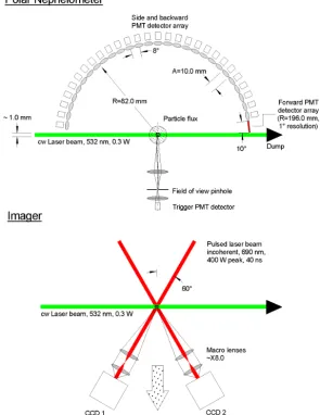
Figure 1.Schematic diagram of the two main components of PHIPS-HALO. The scattering plane of the polar nephelometer (upper diagram) is oriented at 90◦to stereo imager (lower diagram). Note that the forward PMT detector array is no longer used. Figure adapted from Stegmann et al. (2016).
measurements and a different approach is required. To exper-imentally address this question,singleatmospheric ice parti-cles have to besimultaneouslymeasured for both the micro-physics and the corresponding angular light scattering prop-erties.
The Particle Habit Imaging and Polar Scattering probe PHIPS-HALO has been developed to fulfill this requirement. The basic design and operation idea of PHIPS-HALO was presented in the first part of this two paper series (Abdel-monem et al., 2016), denoted by “Part 1” hereafter. In the present paper, the characterization of the instrument in the laboratory is presented (Sect. 2) followed by first results from aircraft deployments in cirrus and Arctic mixed-phase clouds (Sect. 3). The findings are summarized and an outlook is given in Sect. 4.
2 Characterization
2.1 Trigger detector
The trigger detector comprises a two-lens optical system con-sisting of convex lenses with 25 and 40 mm focal lengths and a 7×0.25 mm acrylic glass (PMMA) fiber bundle that is connected to the first channel of the multi-anode photo-multiplier array (MAPMT). The trigger optical system is lo-cated at a polar angle of 90◦ with respect to the scattering plane of the polar nephelometer, but opposite to its detector ring (Fig. 1). The trigger is azimuthally tilted by 32◦out of the scattering plane with a radial distance of the front lens to the laser beam of 24.5 mm. The two-lens system produces an image of the fiber bundle end on the laser beam reduced by about two-thirds, resulting in a field of view (FOV) of the trigger detector of 0.52 mm. Projecting this FOV into the scattering plane, which is perpendicular to the particle trajectory, results in an elliptical FOV with long and short diameters of 0.98 and 0.52 mm, respectively. With this, the sensing area Asa of the instrument can be calculated to be Asa=0.004 cm2. Here, it is important to note that the laser
beam shape is Gaussian with a measured 1/e2 diameter of dl=0.8 mm and a circularity of 0.93 at the position of the
sensing area. This means that the light intensity is nonuni-form across the sensing area, which consequently results in a position-dependent trigger sensitivity. This is disadvanta-geous for sizing and counting particles based on the trigger detector signal. To improve this situation, a beam shaping op-tical element that produces a top hat intensity profile at the sensing area has been designed and will be integrated for fu-ture measurements (see Sect. 4 for details). WithAsaand
as-suming a typical airspeed of 200 m s−1during measurements onboard HALO, a volume sampling rate of 80 cm3s−1is cal-culated. The sensing area of PHIPS-HALO and, therefore, its volume sampling rate, is significantly smaller compared to other imaging probes (e.g., the Cloud Imaging Probe, CIP (DMT, Boulder):Asa=1.6 cm2or the Cloud Particle Imager,
CPI (SPEC Inc., Boulder):Asa=0.04 cm2), but is
compara-ble to the sensing area of conventional single particle light scattering probes (e.g., the Cloud and Aerosol Spectrom-eter, CAS (DMT, Boulder): Asa=0.0025 cm2 or the Fast
Cloud Droplet Probe, FCDP (SPEC Inc., Boulder): Asa=
0.0025 cm2). The reason for this small sensing area used in PHIPS-HALO is that angular light scattering functions are measured on a particle-by-particle basis for typical cloud sit-uations up to 1000 particles cm−3 (see the discussion of the coincidence characteristics below). The Polar Nephelometer (PN) instrument from Laboratoire de Météorologie Physique (LaMP), Université Blaise Pascal, Clermont-Ferrand, France (Gayet et al., 1997) uses a significantly larger sensing area of Asa=0.5 cm2. In contrast to PHIPS-HALO, the PN is
con-structed to measure the angular light scattering function of particle ensembles with the aim that scattering features re-lated to single ice crystals and their specific orientations are averaged out (Gayet et al., 1997). A comparison of further
parameters of PHIPS-HALO with the PN and the CPI are given in Tables 1 and 2 of Part 1, respectively.
The sensing area of PHIPS-HALO was also measured us-ing uniformly sized sus-ingle droplets from a piezo electric droplet generator (GESIM GmbH, Grosserkmannsdorf, Ger-many) mounted on anx-y-z stage. Droplets with a diam-eter of 77±0.1 µm were dispensed at a rate of 1 Hz while slowly moving the dispenser through the sensing area along and across the laser beam. At the same time the signal of the trigger detector was monitored by an oscilloscope. The horizontal and vertical extensions of the sensing area, 1x and1y, were defined by the positions where the trigger sig-nal was reduced to a tenth of its value in the center of the area. With this procedure an extension of 1x=0.53 mm, 1y=0.45 mm was measured resulting in a reduced sens-ing area ofAsa=0.0018 cm2and, consequently, in a reduced
volume sampling rate of 36 cm3s−1compared to the theoret-ical value. While the1xmeasurement is in good agreement with the theoretical value, the1ymeasurement is only about half of the theoretical value, which is a consequence of the Gaussian laser beam profile for this direction.
With these values, the sensing area coincidence probabil-ity, Psa, can be calculated by means of Poisson statistics.
The average number of particles residing in the sensing vol-ume of the instrvol-ument is λ=n·Asa·dl, with n the cloud
particle number concentration. The probability for having more than one particle in the sensing volume at the same time is thenPsa(x >1, λ)=1−(1+λ)·exp(−λ). This
prob-ability is less than 1 % up to particle number concentrations ofn=480 cm−3andn=1000 cm−3for the theoretical and mapped sensing area, respectively.
When a particle is entering the laser beam at the position of the sensing area, part of the scattered light is collected by the trigger detector optics and is guided to the first channel of the MAPMT, where the signal is processed and analyzed. If the trigger event is classified to be a real particle event, the data acquisition is eventually initiated. Details on the trigger signal detection and processing can be found in Part 1.
2.2 Polar nephelometer
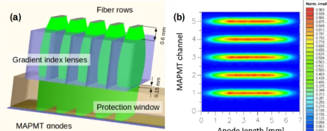
Figure 2.Optical engineering simulations of the redesigned fiber–MAPMT coupler used in the polar nephelometer part of PHIPS-HALO. Optical model(a). Simulated irradiation in the plane of the anode slits of the multi-anode PMT(b).
of the polar nephelometer in the range of 15–20 % was re-vealed by optical engineering calculations and laboratory characterizations (see Sect. 2.1.1 of Part 1). This crosstalk could be clearly attributed to the fact that the numerical aper-ture (NA) and the diameter of the PMMA fibers were too large in combination with the minimum distance to the anode array of the MAPMT constrained by the 1.5 mm thickness of the MAPMT protection window. To solve this crosstalk prob-lem the following redesign of the fiber–MAPMT coupler was performed.
a. The 0.6 mm single PMMA fiber channels were replaced by fiber bundles consisting of 19×0.25 mm PMMA fibers. The individual fibers of the bundle were arranged in a row-like manner at the coupler side in order to (i) uniformly distribute the light across the adjacent an-ode slit and (ii) get a fiber row width that is significantly smaller than the anode width.
b. An array of 32 specifically designed gradient index cylinder lenses were placed between the ends of the fiber rows and the MAPMT protection window. These gradient index lenses (GRINTECH, Germany, model GT-LFCL-100-024-50-NC) have a rod-like shape with a length of 14 mm, a width of 1 mm, and a height of 2.37 mm. The lenses possess anti-reflective coatings on the entrance and exit surfaces, optimized for 532 nm wavelength, and titanium coatings on the long side sur-faces. The latter optically isolate the lenses when they are densely stacked in the coupler. The variation of the refractive index along the width of the lenses ensures, in combination with their height, an optimal focusing of light exiting the fiber ends into MAPMT anodes pro-vided the fiber rows and the index lenses are precisely positioned.
Before a new coupler was manufactured based on these redesign considerations, comprehensive optical engineering simulations were performed to define the optimal distances
Figure 3.Normalized irradiation profiles along(a)and across the anode slits(b)of the MAPMT. The shaded areas in the lower panel indicate the width of the anodes.
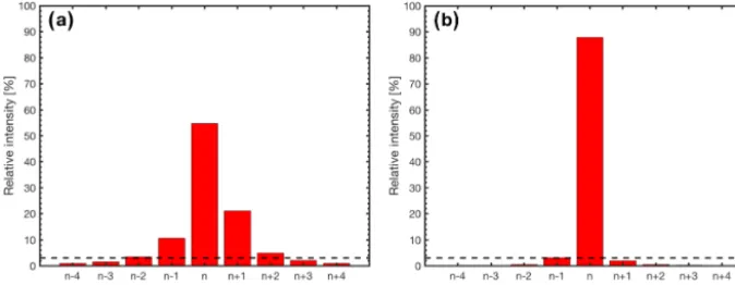
Figure 4.Characterization of the optical crosstalk between adjacent channels of the MAPMT with the old version(a)and the redesigned version of the fiber coupler(b). Note that the manufacturer-specified electrical crosstalk level of 3 % is indicated in the graphs. See text for further details.
illuminated with a gradual decrease of the irradiation towards both ends of the anode. Across the width of the anodes the cylindrical lenses nicely focus the light into the anode area without overlap between the individual focal spots.
The coupler was then manufactured according to the re-sults of the optical engineering simulations and was char-acterized in the laboratory. To take into account the NA of 0.33 of the off-axis parabola mirrors, which is significantly smaller than the NA of 0.39 of the PMMA fibers, the fol-lowing procedure was applied in this characterization. Only one fiber at a time was connected to the 18◦ parabola mir-ror while the connectors of the others were blocked by light tight caps. Water droplets were generated by a pump spray bottle in the vicinity of the instrument inlet and were accel-erated to a speed of about 20 m s−1 by applying a vacuum to the instrument outlet. Scattering data of the droplets was acquired for a short period before the setup was switched to the next fiber. This procedure was repeated until all fibers were connected. The result of this characterization is shown in Fig. 4 where the normalized distribution of the measured intensity in the connected scattering channel (n) and in the neighboring channels (n±1) is shown and contrasted to the crosstalk characterization of the old fiber coupler. The result shows good agreement with the predictions from the opti-cal engineering opti-calculations (Fig. 3) and shows a clear im-provement compared to the old fiber coupler. The remaining mean crosstalk to the neighboring n±1 channels is within the range of the electrical crosstalk of 3 % that is specified by the manufacturer.
The individual fiber bundles are assembled in a densely packed manner in stainless steel ferrules at the side of the parabola mirrors, resulting in a clear aperture of 1.25 mm diameter. This diameter, together with the fiber to mirror and mirror to scattering center distances, results in a FOV of 5.5 mm for the individual channels. The detection volume of the nephelometer channels is then the intersection of this FOV with the laser beam, resulting in a (skewed) cylindrical volume. While the length of the detection volume is equal to
Table 1.Field of view (FOV) areas, detection volumes, and coin-cidence probabilities for the optical arrangement of the polar neph-elometer of PHIPS-HALO. Note that coincidence can be neglected for cirrus but might be considered for mixed-phase cloud condi-tions.
Angle Fiber FOV Detection Coincidence Coincidence
◦ diameter area volume at 10 cm−3 at 100 cm−3
mm cm2 cm3 % %
18 1.25 0.077 0.009 0.4 23
26 1.25 0.055 0.006 0.2 14
34 1.25 0.120 0.005 0.1 9
42 1.25 0.100 0.004 0.1 7
50 1.25 0.088 0.004 0.1 5
58 1.25 0.079 0.003 0.1 4
66 1.25 0.073 0.003 0.1 4
74 1.25 0.070 0.003 0.0 4
82 1.25 0.068 0.003 0.0 3
90 1.25 0.067 0.003 0.0 3
98 1.25 0.068 0.003 0.0 3
106 1.25 0.070 0.003 0.0 4
114 1.25 0.073 0.003 0.1 4
122 1.25 0.079 0.003 0.1 4
130 1.25 0.088 0.004 0.1 5
138 1.25 0.100 0.004 0.1 7
146 1.25 0.120 0.005 0.1 9
154 1.25 0.055 0.006 0.2 14
162 1.25 0.078 0.009 0.4 23
170 1.25 0.132 0.016 1.3 48
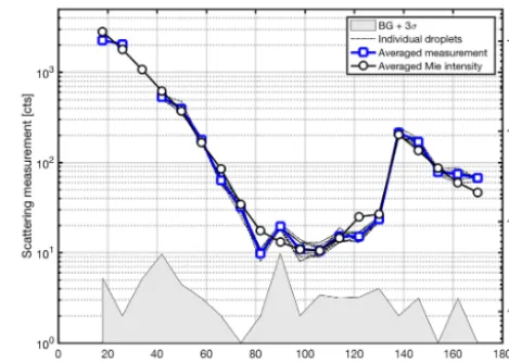
Figure 5. Characterization of the polar nephelometer with dry polystyrene spheres with a nominal monodisperse diameter of 49.7±2.0 µm. The image analysis results were used as input for Mie calculations. The averaged Mie scattering function is shown in black.
Like in Part 1, the response of the improved polar neph-elometer to individual particles passing the (trigger) sens-ing volume was first characterized with NIST-traceable dry polystyrene divinylbenzene particle standards (DRI-CALTM DC-50, Duke Scientific) with a nominal diameter of 49.7±2.0 µm, a standard deviation of 3.4 µm, and a re-fractive index of 1.59 (λ=589 nm). The polystyrene spheres were aerosolized in the vicinity of the instrument inlet and were transported through the optics head by applying a vac-uum to the outlet. Figure 5 shows the measured angular scat-tering functions of 20 individual polystyrene particles. The corresponding mean angular scattering function is compared to the mean theoretical function that was calculated using Mie theory and the cross-sectional equivalent diameter de-duced from the images. For this, the in-house programmed MATLABTM Mie code was used, which was adopted from the Mie code printed in Bohren and Huffman (2007), to cal-culate the angular scattering function of the individually im-aged polystyrene particles. The calculated scattering func-tions were then integrated over the solid angles of the po-lar nephelometer channels. The averaged measured scatter-ing function agrees reasonably well with the averaged func-tion from the Mie simulafunc-tions given the uncertainties in the particle size determination, the refractive index of the par-ticle material, and the position of the parpar-ticle in the laser beam, i.e., the incident light intensity. A significant offset of the measured intensity is observed in the 100–150◦ an-gular range, which might be a consequence of the slightly structured (roughened) surface of the polystyrene spheres in contrast to the Mie model, which assumes a smooth sur-face. Here it is important to note that no corrections have been applied to the measured scattering signals, which
indi-Figure 6.Characterization of the polar nephelometer using uni-formly sized single droplets from a piezo electric droplet generator.
cates rather similar transfer functions for the individual neph-elometer channels.
In the next step, individual droplets from the droplet dis-penser (cf. Sect. 2.1) were analyzed in the same way as de-scribed for the polystyrene standards. The result of this char-acterization is shown in Fig. 6. An even better agreement between measurement and simulation is observed, which is a consequence of a better constrained refractive index for liq-uid water droplets and a more stable position of the particle trajectory through the laser beam. Specifically the steep in-crease of the measured scattering intensity towards the for-ward direction, its minimum between 80 and 120◦, and the edge-like increase of about 10 times at the rainbow angle is nicely mimicked by the Mie simulation. From Fig. 6 clear systematic biases can be detected for the channels 82, 90, and 122◦that will be corrected hereinafter. The bias at 122◦ results in the suppression of the secondary rainbow feature.
It has not yet been possible to compare the improved polar nephelometer of PHIPS-HALO with the aircraft-approved Polar Nephelometer (PN). However, the predecessor PHIPS-HALO nephelometer with the old fiber coupler was com-pared with the PN for ice particle ensembles generated in cirrus simulation experiments in the AIDA (Aerosol Inter-actions and Dynamics in the Atmosphere) cloud chamber (Fig. 7 of Schnaiter et al., 2016). For this comparison the av-eraged angular scattering functions from PHIPS-HALO were corrected for channel crosstalk and channel sensitivity char-acteristics as described in Part 1. A reasonable agreement of both instruments was found, with maximum deviations in the normalized scattering functions of less than 50 %.
2.3 Imaging system
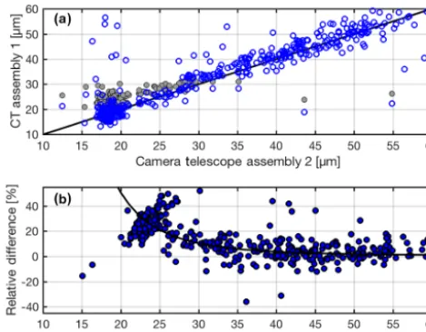
Figure 7.Example of an oversize correction for small particles and a low magnification setting of 4×in camera telescope (CT) assem-bly 1. CT assemassem-bly 2 was set to 6×magnification. For cloud par-ticle sizes smaller than 30 µm, the image analysis algorithm applied to the CT assembly 1 images starts to oversize the particles due to enhanced image blur (gray symbols ina). An oversizing in the range between 10 and 50 % is observed (blue symbols inb). By using the sizing results for CT assembly 2, a correction function can be de-duced to empirically describe this oversizing (black line inb) and to correct the sizes deduced for CT assembly 1 (blue symbols ina).
particle. The magnification of the zoom lenses can be manu-ally set in the range from 1.4×to 9×, which corresponds to field of view dimensions ranging from 6.27×4.72 to 0.98×0.73 mm2, respectively. This allows image acquisition either at the same or at two different fields of view, which is advantageous to avoid a complete failure of the imag-ing system in the case of alignment drifts durimag-ing flight and for cloud situations when small and large ice particles are present at the same time, e.g., in the case of small frozen droplets and large ice crystal aggregates in deep convective outflows (Stith et al., 2014). Consequently, the optical res-olution limit is dependent on the magnification setting and ranges between 7.2 and 2.35 µm for the 1.4×and 9× magni-fication, respectively. Using magnifications of 4×and below results in an oversizing of smaller cloud particles with sizes below about 30 µm that were already identified in Part 1 for glass beads. A correction method for this oversizing is de-scribed in Sect. 2.3.1 together with the strategy used to align the CTA focal distance for aircraft speeds in the laboratory. As there is a large difference between the maximum acqui-sition rates of the CTAs (20 Hz) and the polar nephelome-ter (6 kHz), precautions were taken to have a robust image acquisition procedure in order to achieve an unambiguous assignment of the stereo-microscopic images to the corre-sponding scattering functions. These efforts are presented in Sect. 2.3.2.
2.3.1 CTA characteristics and adjustment
Figure 7 shows a comparison of cloud particle sizes de-duced from the images of the stereo-microscopic imager. The image processing algorithm that is used to deduce mi-crophysical particle properties is described in Schön et al. (2011). The data analyzed for Fig. 7 originate from a cloud chamber experiment where a mixed-phase cloud was gen-erated at a temperature around −20◦C. Details on the ex-perimental procedure applied in such cloud chamber runs can be found in Vochezer et al. (2016). Hence, the data comprise small supercooled liquid droplets, clustered around 20 µm in Fig. 7, as well as larger ice particles. In this ex-periment, the CTAs of PHIPS-HALO were set to magnifi-cations of 4× and 6× for CTA1 and CTA2, respectively. The scatter plot (Fig. 7a) shows an oversizing of CTA1 com-pared to CTA2 for particle sizes smaller than about 30 µm, which is more clearly reflected in the relative size difference (CTA1-CTA2)/CTA2·100 %, shown in Fig. 7b. Thus the dif-ference in the optical resolution limits of∼5.3 µm (4×) and ∼3.5 µm (6×) results in an enhanced blur in the 4×images and, consequently, in an oversizing of the particles by the image processing algorithm. Fitting an empirical function to the relative size difference allows for the size correction of the particles imaged by CTA1.
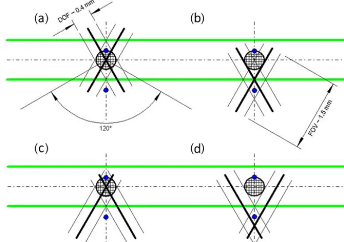
Figure 8.Schematics of the alignment strategy for the zoom lens focus. Ideal overlap between the two zoom lens fields of view (FOVs) and the trigger sensing area(a). The trigger sensing area is represented by the hatched area centered in the laser beam diameter (the edges of the laser beam are indicated by the green lines). The positions of the particle when entering the sensing area and after the camera shutter delay are shown as blue dots, assuming an airspeed of 200 m s−1. Note that the particle is already at the edge of the FOV and outside the depth of field (DOF) of both zoom lenses when the camera shutters open. Displacement of the FOVs relative to the sensing area by about 0.4 mm to compensate for the particle movement during the shutter delay(b). Zoom lens focus adjustment on a slowly moving particle in the laboratory(c). Focus adjustment on a fast moving particle during aircraft measurements(d).
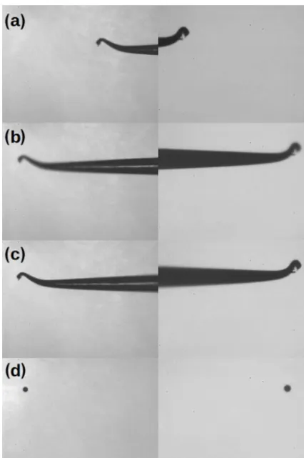
side of the trigger sensing area, the trigger optics were back-lit while a tungsten needle was slowly moved along the in-strument axis until the tip was shining up at the front edge of the trigger FOV. In this situation, the tip of the tungsten nee-dle should be located on the inner (entrance) side of the FOV of both CTAs (Fig. 9a). With the delay for the illumination flash, which has to be set to at least 4 µs to ensure the cam-era shutters are open before the flash laser is triggered, and the expected typical airspeed, e.g., 250 m s−1, the tungsten needle can be moved accordingly along the instrument axis to mark the particle position at the time when the flash laser is triggered (Fig. 9b). The focal plane of the CTAs can then be adjusted to this depth (Fig. 9c). This alignment procedure can be cross-checked in the laboratory using slowly moving water droplets (cf. Sect. 2.2) and setting the camera shutter and illuminating trigger delays to values large enough so that the particle has the same displacement as expected under fast flight conditions. Figure 9c gives an example stereo image that was acquired during such a laboratory test, showing that the presented alignment procedure put the focal planes of the CTAs at the correct depth.
Depending on the magnification settings, the CTAs cover different FOVs and DOFs, resulting in different volumes that are captured in the images. For typical magnification settings of 4×and 6×observation, volumes of 0.9 and 0.3 mm3
re-sult, respectively, which is small enough to avoid any signif-icant particle coincidence up to particle number concentra-tions of about 200 cm−3.
2.3.2 Assignment of the images to the corresponding angular scattering functions
cam-Figure 9. Stereo images of the tungsten needle taken during the alignment procedure described in Sect. 2.3.1. Needle at the edge of the trigger FOV(a). Needle tip marks the particle position when the CTA shutters have been opened and the illumination flash is fired at an assumed airspeed of 250 m s−1(b). Focal planes of the CTAs have been adjusted to position (depth) of the needle tip(c). Cross-check of the alignment with slowly moving water droplets in the laboratory using a illumination trigger delay scaled to the differ-ences in airspeed between laboratory and aircraft operation(d).
era busy signals are routed to the FPGA. If either one or both busy signals are high no camera trigger is sent and registered. Further, to give the instrument computer enough time to re-ceive and store the stereo images, an additional post-trigger period can be defined by the user, within which camera trig-gers and registrations are suppressed. With the current hard-ware and softhard-ware, a post-trigger period of 300 ms has to be set in order to avoid image losses.
With these precautions there are usually as many camera trigger registrations in the scattering data set as number of stereo images stored on the solid state disk, which makes the image assignment straightforward. Occasionally, there is a mismatch between these numbers, which makes the assign-ment of the stereo images to the corresponding scattering function more challenging. However, also in these situations an assignment of at least a part of the acquired images be-comes possible by a procedure, where the time stamp
dif-ferences between all scattering data sets with a camera trig-ger register (1ts) are compared to the time stamp differences
between all acquired stereo images (1ti). If the difference
of these two differences (1t t=1ts−1ti) matches within
a reasonable limit (±50 ms), a stereo image is assigned to a scattering data set. Otherwise either a stereo image is miss-ing (1t t <−50 ms) and a padding element is inserted in the camera data array, or, in the case that a scattering data set is missing (1t t >+50 ms), the stereo image is excluded.
2.4 Electronics
PHIPS-HALO possesses a set of specifically designed elec-tronics boards for signal detection, signal conditioning and conversion, and acquisition control. Brief introductions of these boards in conjunction with a detailed step-by-step de-scription of the signal detection and processing sequence can be found in Part 1. For the characterization presented in this section, it is important to resume the backplane con-troller board, which consists of a 48 MHz system concon-troller FPGA (Xilinx, model Spartan 2) and a 16k by 18 bits FIFO memory (IDT72V265) to buffer the scattering data prior to being read by the USB daughter board (Bitwise Systems, model QuickUSB) for transferring the data to the instrument computer (ADL Embedded Solutions, model ADL945PC-T7400). Although the FIFO is 18 bits wide, only 16 bits are used to define one word.
Prior to the start of the data acquisition, the FPGA is pro-grammed by sending a .bit file from the instrument computer to the FPGA. This program then handles the data acquisition and buffering in the FIFO as detailed in Part 1. Each particle data set consists of 38 words, so the FIFO can buffer a to-tal of 421 particle data sets. While the polar nephelometer part of PHIPS-HALO has a maximum data acquisition rate of 13 kHz (see below), the image acquisition system, i.e., the CCD cameras, have a maximum (specified) acquisition rate of only 20 Hz. Therefore, in order to not lose scattering data sets that might have corresponding images, the FPGA stops particle data acquisition in situations when the particle rate is high and the FIFO might be completely filled up before it is emptied by an USB read. Communication between the backplane board and the instrument computer is established by the USB daughter board that comes with a software li-brary for developing custom applications. New data acqui-sition software, composed of a scattering data read applica-tion and an image receiving and storing applicaapplica-tion was de-veloped based on the QuickUSB library (QuickUSB Library v2.15.2, Bitwise Systems) and the library that comes with the CCD camera (Vimba v1.4, Allied Vision Technologies).
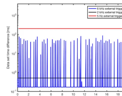
tional delays by simultaneously handling the image trans-fer. A maximum continuous scattering data acquisition rate of 12 kHz was determined only intermittent for about 140 µs when the FIFO was read and transferred via the USB daugh-ter board (set to 32 ms in these tests). In a second test the im-age acquisition software was also running during the pulse rate measurements over a fixed period of 20 s. The result of this test is depicted in Fig. 10 where the time difference be-tween consecutive data sets is plotted for three different pulse rates. While for 5 Hz and 2 kHz cases the time difference is constant and equal to the inverted frequency, the time analy-sis of the scattering data set for 6 kHz shows infrequent de-lays between consecutive data sets up to 100 ms. A total of 55 data sets have a time difference longer than the 0.167 ms defined by the set pulse rate. Consulting the number of ac-quired images of 67, it is obvious that the image acquisition process holds the scattering data read process until the ac-quired images (two per camera trigger) have been transferred to the solid state disk. This often results in a full FIFO, a stop of scattering data acquisition, and, consequently, in a loss of data sets. Further investigations revealed a maximum parti-cle acquisition rate of 3.5 kHz without any loss in the scat-tering as well as image data. Using the volume sampling rate of 36 cm3s−1 at 200 m s−1 airspeed (Sect. 2.1), this facili-tates a maximum particle concentration of about 100 cm−3 that can be continuously acquired without any loss.
In a final test, the acquisition dead time after individual trigger events was investigated by applying a train of double pulses with decreasing time lag. This test revealed a dead time of about 12 µs that is required by the electronics for pulse analysis and analog-to-digital conversion of each of the 32 channels followed by a successive read of the con-verted signals by the FPGA. Assuming again an airspeed of 200 m s−1, this results in a minimum particle distance of 2.4 mm that can be resolved by the electronics, meaning that the post-trigger data processing is fast enough to per-form a shattering analysis based on the inter-particle arrival times – at least for cirrus cases.
Figure 10.Characterization of the maximum scattering data acqui-sition rate of PHIPS-HALO in the case of simultaneous image ac-quisition at 3 Hz. Note that the maximum rate without a simultane-ous image acquisition is 12 kHz.
3 First results
In this section first results from aircraft measurements with PHIPS-HALO are presented. Although the instrument de-puted on the HALO aircraft in the missions ML-CIRRUS (Voigt et al., 2016) and ACRIDICON-CHUVA (Wendisch et al., 2016) in 2014, the examples that are given below are from two recent aircraft projects, namely within the ARISTO program conducted with the NSF/NCAR GV HI-APER (Gulfstream-V High-performance Instrumented Air-borne Platform for Environmental Research) in February and March 2017 and the ACLOUD mission conducted with the AWI Polar 6 aircraft of the Alfred Wegener Institute in May and June 2017. The reason for this confinement is that the full instrument capabilities including a crosstalk-free scatter-ing function measurement and a reliable image-to-scatterscatter-ing function correlation were only available in these recent mis-sions. First results from the ACRIDICON-CHUVA mission are presented elsewhere (Wendisch et al., 2016; Järvinen et al., 2016).
test flight a marine boundary layer cloud deck west of Cali-fornia was probed.
The Arctic CLoud Observations Using airborne measure-ments during polar Day (ACLOUD) mission took place from 22 May to 28 June 2017 based in Longyearbyen (Svalbard, Norway). Within ACLOUD, PHIPS-HALO participated in 17 research flights north and west of Svalbard. In these flights PHIPS-HALO collected a unique data set of the microphys-ical and light scattering properties of ice in Arctic stratiform clouds.
3.1 Stereo-microscopic image examples
Before results of the correlated microscopic and angular light scattering measurements are presented, examples of the stereo imaging method are shown to document the qual-ity and information content that can be expected from the PHIPS-HALO imagery acquired under flight conditions. It is important to emphasize here that the stereo imaging method is essential for the overall concept of PHIPS-HALO as it is the basis for the interpretation of single particle angular scattering functions. The method not only provides a three-dimensional impression of the imaged particle, but also gives its orientation with respect to the scattering plane. Both infor-mation parts are necessary to represent the particle in optical models for simulating its angular light scattering function.
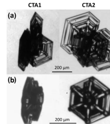
A general problem in two-dimensional optical imaging of ice crystals – even in the case of real in-focus optical microscopy like that used in PHIPS-HALO – is that there are always parts of the particle obscured in the image that makes a representation of its three-dimensional geometric structure impossible. In Fig. 11 two examples of skeleton plates are depicted that were sampled by PHIPS-HALO dur-ing ACLOUD in ice precipitation underneath a mid-level cloud at temperatures between −10 and −14◦C. These ex-amples nicely demonstrate how the stereo imaging method enhances the microphysical information that can be drawn from the PHIPS-HALO stereo-micrographs of individual ice crystals. The stereo image examples shown in Fig. 11 reveal that these crystals are actually composed of multiple stacked skeleton plates. In example (b) three hexagonal plates are concentrically stacked along the basal facet, which becomes obvious by inspecting the image of CTA1 (left). If only the image of CTA2 (right) were available, the crystal would have been classified most likely as a single skeleton plate. Al-though a stacked plate arrangement is identifiable in CTA2 of example (a), the one side plane that is radiating in a dif-ferent direction becomes visible only by imaging the crys-tal under a different viewing angle as in the case of CTA1. Note that a stereo imaging approach is also used in the 2D-S probe (Two-dimensional Stereo Probe, SPEC Inc., Boulder) in which two independent shadowgraph images of the same particle are recorded at a viewing distance of 90◦. The exam-ples given in Fig. 11 also show that the enhanced bright field image clarity due to the use of incoherent and
monochro-Figure 11.Two examples of stereo images for plate-like ice crystals captured in ice precipitation underneath an Arctic mid-level cloud. Images captured in the Camera Telescope Assembly 1 (CTA1) are depicted on the left side; the corresponding images of the same crys-tal captured in CTA2 are shown on the right side. The examples nicely show the advantage of having a second view of the crystal.
matic light as documented in the laboratory versions (Ab-delmonem et al., 2011; Schön et al., 2011) is also achieved under flight conditions.
An additional feature of stereo-microscopic imaging is the possibility of using different magnifications for the two images. Different magnifications result in different FOVs, which enables the imaging of large and small ice particles at the same time without having the problem that large crys-tals are not completely captured in a narrow FOV. Further, a larger FOV of one CTA also enables the capture of coinci-dent particles and possible breakup events of large ice parti-cles or aggregates in a single frame.
3.2 Single particle angular scattering functions
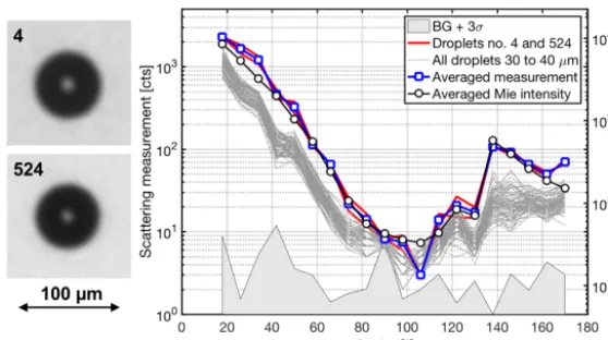
trig-Figure 12.Test of the automatic image-to-scattering function assignment procedure. Sparsely imaged large diameter droplets with similar diameters of 64 and 66 µm were selected from the PHIPS-HALO imagery collected in a 12 min flight leg in a marine boundary layer cloud. The images (with numbers 4 and 524 in image) were automatically assigned to the particle trigger events no. 738 and 3986 of the angular light scattering data set (red lines). The data set numbers correspond to a time difference of about 10 min between the two trigger events. The averaged scattering function of these two events (blue) can be nicely reproduced by Mie calculations for a single droplet with a diameter of 65 µm (black). Single particle angular light scattering functions are assigned to those droplets from the imagery that have a diameter between 30 and 40 µm (dashed-dotted lines).
gers from significantly smaller particles. Further, by select-ing the two images with the largest difference in time, the robustness of the assignment method against time-related in-fluences can be checked. The two imaged droplets in Fig. 12 with image numbers 4 and 524 have diameters of 66 and 64 µm, respectively, and were captured with a time differ-ence of almost 10 min. Figure 12 shows the scattering func-tions that were automatically assigned to these images by the assignment procedure. As expected for nearly equal-sized droplets, the scattering functions show almost no difference, which is clear proof of a successful image-to-scattering func-tion assignment. The two scattering funcfunc-tions were then av-eraged and compared with the result of a Mie calculation for a droplet with 65 µm diameter. Again, an excellent agreement is achieved, which shows that the scattering function mea-surement is also reliable under flight conditions.
The correlated measurement of microphysical and angu-lar light scattering properties on a single particle basis gives unprecedented research opportunities in the field of cloud physics. The correlated data can be compiled as single (ice) particle data or as habit-specific and phase-specific averaged data. Examples of single ice particle data will be given in the remainder of this section. Averaged data are presented in Sect. 3.3.
Figure 13 gives single particle angular scattering func-tions measured for two plate-like ice particles during the ARISTO2017 project. These two plates were selected be-cause (i) they have a similar size and (ii) they are similarly oriented, though the orientation of their c-axes differs by at least 10◦in the horizontal plane. An inspection of the stereo images reveals that crystal (b) appears darker than crystal (a). A darker appearance of a nonabsorbing object in bright field
microscopy is the consequence of more object–air interface interactions of the light rays that incide and penetrate the ob-ject. This means that, in the case of the ice crystals shown in Fig. 13, crystal (b) likely has more surface distortions in terms of steps, roughness, indentations, and air inclusions compared to crystal (a), which appears more transparent. As a consequence of this structural difference, the angular light scattering properties of the two crystals differ in terms of a higher fraction of diffuse light scattering (reflection) in the case of the more structured crystal (b) compared to the less structured crystal (a). The corresponding measured angular light scattering functions of the two crystals, shown on the right side of Fig. 13, support this conclusion. Crystal (b) in-duces scattering intensities measured in the side and back-ward directions that exceed those of the less structured crys-tal (a) by up to 1 order of magnitude. It is acknowledged, however, that detailed light scattering simulations, like in the work of Shcherbakov et al. (2006), are necessary to un-ambiguously prove that the observed differences can be at-tributed to differences in the ice crystal complexity.
Figure 13.Stereo images of two plate-like crystals captured during the ARISTO2017 project (left). Maximum crystal dimensions are 132 and 167 µm for crystal (a) and (b), respectively. Correlated angular scattering functions measured for the two crystals are shown (right). Note the 26 and 154◦local maxima in the case of the more pristine crystal (a).
3.3 Averaged angular scattering functions
While the previously shown single particle angular light scat-tering functions are of high value for understanding the fun-damental light scattering properties of atmospheric ice parti-cles, cloud angular scattering functions averaged over many single particle measurements are of more interest when it comes to the radiative impact of the clouds on the energy budget of the atmosphere. Despite the common method of a separate analysis of the microphysical and scattering en-semble data, the correlated single particle data from PHIPS-HALO also facilitate unprecedented analysis methods in the case of cloud ensemble data. These novel capabilities are pre-sented in the following two sections.
3.3.1 Habit-specific angular scattering functions from ice clouds
The correlated single particle image and scattering data pro-vided by PHIPS-HALO can be used to calculate habit-specific averaged ice particle ensemble data, even in situa-tions when the cloud is not homogeneous and composed of ice crystals with different habits. To highlight this unique ca-pability, a flight leg from RF02 of ∼30 min, conducted on 24 February 2017 during the ARISTO-2017 project, was an-alyzed. In this leg, the GV aircraft probed an extensive cloud field over west and central Nebraska.
In a first analysis, bullet rosettes (see Fig. 14) were manu-ally selected from the PHIPS-HALO imagery that was cap-tured between 20:36 and 20:43 UT when the aircraft de-scended from an initial altitude of 7.7 to 6.7 km. During this descent the GV profiled a thin cirrus layer, which existed at ambient temperatures between −47 and−41◦C. The cloud was dominated by hollow columns and hollow bullet rosettes with minor fractions of irregular particles and rosettes with
side planes. Only crystals that could be clearly classified as (hollow) bullet rosettes, i.e., excluding crystals with side planes, were selected from the PHIPS-HALO stereo imagery, resulting in a total number of 54 selected crystals (see Fig. 14 for examples). The individual angular scattering functions assigned to this set of selected crystals are plotted on the right of Fig. 14 together with the habit-specific averaged angular scattering function of this crystal class.
In a second analysis, plate-like crystals were manually se-lected from the period 20:52 to 21:00 UT when a thicker altostratus cloud was profiled between 5.4 and 4.4 km al-titudes. The temperatures in this cloud were significantly warmer and ranged between−31◦C at cloud top and−26◦C at the bottom of the cloud. The ice crystal habit distribu-tion was much broader in this cloud compared to the thin cirrus case, with plate aggregates and side planes but also with significant numbers of columns, rosettes, rimed parti-cles, and small irregular particles. Again, only crystals with a clear plate and side plane habit were selected from the PHIPS-HALO imagery, resulting in a total number of 17 se-lected crystals (see Fig. 15 for examples). The individual an-gular scattering functions assigned to these crystals and the habit-averaged ensemble scattering function are plotted on the right of Fig. 15.
Figure 14.Examples of hollow bullet rosettes selected from the imagery captured by PHIPS-HALO during the descent through a cirrus cloud of ∼ −45◦C over Nebraska. Measured single particle angular light scattering functions automatically assigned to the selected hollow bullet rosettes (right, dashed-dotted lines). The habit-specific averaged angular scattering function of this particle class is given in red.
Figure 15.Same as in Fig. 14 but for plate-like and side plane crystals selected from the imagery captured by PHIPS-HALO during the descent through an altostratus cloud od ∼ −28◦C over Nebraska.
PHIPS-HALO to answer the question of which microphysi-cal property of ice clouds dominates their angular light scat-tering behavior – the crystal habit or the crystal complexity in terms of distortions, inclusions, and surface roughness. This will be the subject of future studies after PHIPS-HALO has participated in further cloud-related aircraft projects.
3.3.2 Phase-specific angular scattering functions from mixed-phase clouds
Figure 16.Example of PHIPS-HALO data acquired in a low-level Arctic stratus cloud. Bright field microscopic images of liquid droplets and ice particles are grouped on the left. The angular scattering functions of the corresponding droplets (blue) and ice crystals (red) are plotted on the right. Averaged scattering functions of each particle class are given by blue and red symbols. The averaged theoretical light scattering function from Mie theory is given by black symbols. Note that the averaged function of the ice crystals (red symbols) is clearly distinct from the corresponding function of the liquid droplets (blue symbols) for scattering angles larger than 50◦. Two scattering functions from the ice particle class are labeled with the corresponding image number to emphasize this unique feature of PHIPS-HALO.
profiled a low-level arctic stratus cloud that was approxi-mately 200 m thick, northwest (81◦150N, 9◦150E) of Sval-bard, Norway. The temperature within the cloud ranged be-tween−1◦C at cloud base and−4◦C at the cloud top. The trigger threshold of PHIPS-HALO again was set in a way that the instrument started to trigger on droplets with diam-eters larger than 30 µm. The stereo imagery acquired clearly revealed the presence of some drizzle drops, with sizes up to 150 µm located near the cloud top where small hollow columns were observed. The observed ice crystal habits were columnar throughout the cloud with needles, aggregates of needles, and hollow columns – all with different degrees of surface roughness and riming.
The corresponding angular scattering functions of the im-aged droplets are narrowly grouped, with the primary and secondary rainbows clearly indicated at the 138 and 122◦ de-tection angles, respectively (inset of Fig. 16). The droplet di-ameters deduced from the stereo images are used in Mie the-ory to calculate the averaged angular scattering function of this particle ensemble that nicely mimics the average of the measured functions. Scattering functions from ice particles are more varying but have a rather flat angular dependence, which is likely the consequence of significant single parti-cle complexity in terms of hollowness, surface roughness, and riming. Consequently, the resulting averaged scattering function of the imaged ice particle ensemble shows a flat and featureless angular dependence and is clearly distinct from the corresponding function of the droplets for scattering an-gles larger than 50◦. Interestingly, the averaged scattering
function of these mixed-phase ice particles does not signifi-cantly differ from the corresponding habit-specific functions presented in the previous section, even though those crys-tals were measured in a completely different atmospheric compartment. However, further measurements and analyses are necessary to clarify whether this observation is a general property of atmospheric ice particle ensembles.
4 Summary and outlook
number of out of focus images in the case of large ice crys-tals.
Author contributions. MS is leading the development of PHIPS-HALO and acquired the necessary funds. MS designed the MAPMT fiber coupler and performed the optical engineering calculations. MS and EJ did the further technical improvements, characterized PHIPS-HALO in the laboratory, deployed the instrument in aircraft projects, and analyzed the results. AA was involved in the instru-ment design and assembled the first version of PHIPS-HALO. TL supported the work by additional funding. MS wrote the manuscript with comments from all co-authors.
Data availability. All laboratory and field data presented in this pa-per are available upon request from the corresponding author ([email protected]).
Competing interests. The authors declare that they have no conflict of interest.
Acknowledgements. The authors would like to express their grati-tude to the technical crews at IMK-AAF, at the Research Aviation Facility of NCAR, and at AWI for their support in certifying and integrating PHIPS-HALO to the different airborne platforms. Dirk Kalmbach from AWI and Guillaume Mioche from LaMP, France are thanked for their technical help and their support in operating PHIPS-HALO in ACLOUD. This work was funded within the Helmholtz Research Program Atmosphere and Climate and by the German Research Foundation (DFG grants SCHN 1140/1-1, SCHN 1140/1-2, and SCHN 1140/3-1) within the DFG priority program 1294 (HALO). The National Science Foundation (NSF) is thanked for providing access to the NSF/NCAR C-130 and HIA-PER aircrafts during the ARISTO 2016 and ARISTO 2017 projects. The German Research Foundation is thanked for providing access to the AWI Polar-6 aircraft during the ACLOUD project as part of the Transregional Collaborative Research Center TR172 (AC3). The article processing charges for this open-access
publication were covered by a Research Centre of the Helmholtz Association.
2011, 2011.
Abdelmonem, A., Järvinen, E., Duft, D., Hirst, E., Vogt, S., Leisner, T., and Schnaiter, M.: PHIPS–HALO: the airborne Particle Habit Imaging and Polar Scattering probe – Part 1: Design and operation, Atmos. Meas. Tech., 9, 3131–3144, https://doi.org/10.5194/amt-9-3131-2016, 2016.
Baran, A. J.: From the single-scattering properties of ice crystals to climate prediction: a way forward, Atmos. Res., 112, 45–69, https://doi.org/10.1016/j.atmosres.2012.04.010, 2012.
Baum, B. A., Yang, P., Hu, Y. X., and Feng, Q. A.: The impact of ice particle roughness on the scattering phase matrix, J. Quant. Spectrosc. Ra., 111, 2534–2549, 2010.
Baumgardner, D., Abel, S. J., Axisa, D., Cotton, R., Crosier, J., Field, P., Gurganus, C., Heymsfield, A., Korolev, A., Krämer, M., Lawson, P., McFarquhar, G., Ulanowski, Z., and Um, J.: Cloud Ice Properties: In Situ Mea-surement Challenges, Meteorol. Monogr., 58, 9.1–9.23, https://doi.org/10.1175/AMSMONOGRAPHS-D-16-0011.1, 2017.
Bohren, C. F. and Huffman, D. R.: Absorption and Scattering of Light by Small Particles, Wiley-VCH Verlag GmbH, Weinheim, 2007.
Gayet, J. F., Crepel, O., Fournol, J., and Oshchepkov, S.: A new airborne polar nephelometer for the measurements of optical and microphysical cloud properties. Part 1: Theoretical design, Ann. Geophys., 15, 451–459, https://doi.org/10.1007/s00585-997-0451-1, 1997.
Gayet, J. F., Ovarlez, J., Shcherbakov, V., Ström, J., Schumann, U., Minikin, A., Auriol, F., Petzold, A., and Monier, M.: Cir-rus cloud microphysical and optical properties at southern and northern midlatitudes during the INCA experiment, J. Geophys. Res.-Atmos., 109, 1–13, https://doi.org/10.1029/2004JD004803, 2004.
Järvinen, E., Schnaiter, M., Mioche, G., Jourdan, O., Shcherbakov, V. N., Costa, A., Afchine, A., Krämer, M., Heidelberg, F., Jurkat, T., Voigt, C., Schlager, H., Nich-man, L., Gallagher, M., Hirst, E., Schmitt, C., Bansemer, A., Heymsfield, A., Lawson, P., Tricoli, U., Pfeilsticker, K., Vochezer, P., Möhler, O., and Leisner, T.: Quasi-spherical ice in convective clouds, J. Atmos. Sci., 73, 3885–3910, https://doi.org/10.1175/JAS-D-15-0365.1, 2016.
Schnaiter, M., Järvinen, E., Vochezer, P., Abdelmonem, A., Wagner, R., Jourdan, O., Mioche, G., Shcherbakov, V. N., Schmitt, C. G., Tricoli, U., Ulanowski, Z., and Heymsfield, A. J.: Cloud chamber experiments on the origin of ice crystal com-plexity in cirrus clouds, Atmos. Chem. Phys., 16, 5091–5110, https://doi.org/10.5194/acp-16-5091-2016, 2016.
Schön, R., Schnaiter, M., Ulanowski, Z., Schmitt, C., Benz, S., Möhler, O., Vogt, S., Wagner, R., and Schurath, U.: Particle habit imaging using incoherent light: a first step toward a novel instru-ment for cloud microphysics, J. Atmos. Ocean. Tech., 28, 493– 512, 2011.
Shcherbakov, V., Gayet, J.-F., Baker, B., and Lawson, P.: Light scat-tering by single natural ice crystals, J. Atmos. Sci., 63, 1513– 1525, https://doi.org/10.1175/JAS3690.1, 2006.
Smith, H. R., Webb, A., Connolly, P., and Baran, A. J.: Cloud chamber laboratory investigations into the scattering properties of hollow ice particles, J. Quant. Spectrosc. Ra., 157, 106–118, https://doi.org/10.1016/j.jqsrt.2015.02.015, 2015.
Stegmann, P. G., Tropea, C., Järvinen, E., and Schnaiter, M.: Com-parison of measured and computed phase functions of individual tropospheric ice crystals, J. Quant. Spectrosc. Ra., 178, 379–389, https://doi.org/10.1016/j.jqsrt.2015.12.019, 2016.
Stith, J. L., Avallone, L. M., Bansemer, A., Basarab, B., Dorsi, S. W., Fuchs, B., Lawson, R. P., Rogers, D. C., Rut-ledge, S., and Toohey, D. W.: Ice particles in the upper anvil regions of midlatitude continental thunderstorms: the case for frozen-drop aggregates, Atmos. Chem. Phys., 14, 1973–1985, https://doi.org/10.5194/acp-14-1973-2014, 2014.
Ulanowski, Z., Hesse, E., Kaye, P. H., and Baran, A. J.: Light scat-tering by complex ice-analogue crystals, J. Quant. Spectrosc. Ra., 100, 382–392, 2006.
Vochezer, P., Järvinen, E., Wagner, R., Kupiszewski, P., Leis-ner, T., and Schnaiter, M.: In situ characterization of mixed phase clouds using the Small Ice Detector and the Parti-cle Phase Discriminator, Atmos. Meas. Tech., 9, 159–177, https://doi.org/10.5194/amt-9-159-2016, 2016.
Voigt, C., Schumann, U., Minikin, A., Abdelmonem, A., Af-chine, A., Borrmann, S., Boettcher, M., Buchholz, B., Bugliaro, L., Costa, A., Curtius, J., Dollner, M., Dörnbrack, A., Dreiling, V., Ebert, V., Ehrlich, A., Fix, A., Forster, L., Frank, F., Fütterer, D., Giez, A., Graf, K., Grooß, J.-U., Groß, S., Heimerl, K., Heinold, B., Hüneke, T., Järvinen, E., Jurkat, T., Kaufmann, S., Kenntner, M., Klingebiel, M., Kli-mach, T., Kohl, R., Krämer, M., Krisna, T. C., Luebke, A., Mayer, B., Mertes, S., Molleker, S., Petzold, A., Pfeilsticker, K., Port, M., Rapp, M., Reutter, P., Rolf, C., Rose, D., Sauer, D., Schäfler, A., Schlage, R., Schnaiter, M., Schneider, J., Spel-ten, N., Spichtinger, P., Stock, P., Walser, A., Weigel, R., Weinzierl, B., Wendisch, M., Werner, F., Wernli, H., Wirth, M., Zahn, A., Ziereis, H., and Zöger, M.: ML-CIRRUS: the air-borne experiment on natural cirrus and contrail cirrus with the high-altitude long-range research aircraft HALO, B. Am. Me-teorol. Soc., 98, 271–288, https://doi.org/10.1175/BAMS-D-15-00213.1, 2016.