https://doi.org/10.5194/amt-10-3103-2017 © Author(s) 2017. This work is distributed under the Creative Commons Attribution 3.0 License.
Using paraxial approximation to describe the optical setup of a
typical EARLINET lidar system
Panagiotis Kokkalis
Institute of Astronomy, Astrophysics, Space Applications and Remote Sensing, National Observatory of Athens, 15236, Greece
Correspondence to:Panagiotis Kokkalis ([email protected]) Received: 9 July 2016 – Discussion started: 2 August 2016
Revised: 3 June 2017 – Accepted: 10 July 2017 – Published: 25 August 2017
Abstract. The mathematical formulation for the optical setup of a typical EARLINET lidar system is given here. The equations describing a lidar system from the emitted laser beam to the projection of the telescope aperture on the fi-nal receiving unit (i.e., photomultiplier or photodiode) are presented, based on paraxial approximation and geometric optics approach. The receiving optical setup includes a tele-scope, a collimating lens, an interference filter and the en-semble objective eyepiece. The set of the derived equations interconnects major parameters of the optical components (e.g., focal lengths, diameters, angles of incidence), reveal-ing their association with the distance of full overlap of the system. These equations may used complementarily with an optical design software, for the preliminary design of a sys-tem or can be used as a quick check up tool of an existing lidar system. The evaluation of the formulation on a real sys-tem is performed with ray-tracing simulations, revealing an overall good performance with relative differences of the or-der of 5 % mainly attributed to the limitations of the thin lens approximation.
1 Introduction
Lidars are efficient tools for retrieving the aerosol optical and microphysical properties in the planetary boundary layer (PBL) and free troposphere. More precisely, the lidar tech-niques that are widely used for aerosol research are ca-pable of providing range-resolved information for (a) the aerosol backscatter coefficient(βαer)using the backscatter
li-dar technique (e.g., Fernald et al., 1972; Klett, 1981), (b) the aerosol extinction coefficient (ααer) using the Raman lidar
opti-cal performance and control the quality of aerosol measure-ments, a number of quality assurance (QA) tests have been adopted and applied in EARLINET lidar systems (Freuden-thaler, 2008). Moreover, increased effort has been made by the European lidar community to develop and apply accurate depolarization calibration techniques (Freudenthaler, 2016) and quantify and correct the influence of systematic error in-troduced by imperfections of lidar optical elements on the depolarization related retrievals (Mattis et al., 2009; Bravo-Aranda et al., 2016; Belegante et al., 2016). These studies are based on the description of the state of polarization of light and lidar optical elements by means of the Müller– Stokes formulation. The present study tackles basic lidar de-sign trade-offs, and more advanced topics such as depolar-ization measurements are out of its scope.
The lidar equation in its simplest form includes the over-lap function (O(z))and the overall optical efficiency of the system. The overlap function is range-dependent and thus re-lated to the lidar system geometry, since it describes the frac-tion of the light scattered within the receiver field of view, taking values from 0 to 1 (Wandinger, 2005). More precisely, at the height range where the overlap function reaches the value of 1, each point of the telescope aperture collects the scattered light entirely and with the same efficiency (Fig. 1a). This height range is determined by the intersection point be-tween the outer edge of the laser beam divergence (LBD) and the lateral surface of receiver field of view (RFOV) cone, with the apex on the point of the telescope aperture farthest away from the laser (Fig. 1a). This range is known as the dis-tance of full overlap (DFO) and is usually found from 500 to 1500 m for EARLINET aerosol lidar systems. The over-lap function depends on the range up to the DFO, adding a significant drawback to the retrieval of aerosol optical prop-erties from lidar systems, since it becomes difficult to ob-tain useful and accurate information regarding the aerosol present below that height range. More precisely, Wandinger and Ansmann (2002) demonstrated that when not applying overlap correction in lidar signals, the retrieved aerosol ex-tinction coefficient may take even non-physical negative val-ues for heights up to the DFO. However, they proposed that the effect of the incomplete overlap can be corrected, and trustworthy retrievals may finally be obtained in the case of a system operating both elastic and Raman channels under the assumption that they are affected by the same overlap func-tion.
Thus, in order to optimize the performance of a lidar at lower altitudes and effectively retrieve optical properties of the aerosol entrapped below the PBL height, it is of great importance that the receiving telescope is able to detecting the emitted laser pulse, already at short ranges from the li-dar system. Therefore, a low full overlap height is needed. The wide-angle RFOV is not an optimal solution for mini-mizing the DFO, since in that case (a) the signal will be con-taminated with more sky background light, and (b) multiple scattering effects have to be taken into account, especially
for case studies of optically thick targets (i.e., water and ice clouds; e.g., Eloranta, 1998; Wandinger, 1998). Nevertheless, there are systems employing two telescopes, one for the short ranges and the other for the far ones, with the short-range one having a wider RFOV angle (e.g., Engelmann et al., 2016). However, such setups are more complicated and their sig-nals demand special treatment during the retrieval processing schemes.
Case studies, but also long-term lidar observations per-formed during the last decade at various EARLINET sta-tions, revealed that the DFO have to be much lower than 600 m in order to detect the boundary layer at European latitudes, especially during wintertime (e.g., Matthias and Bösenberg, 2002; Matthias et al., 2004; Amiridis et al., 2007; Baars et al., 2008). Measurements of the aerosols within the PBL are in particular required during daytime, when the con-vection is stronger. However, daytime lidar operation suffers from the increased sky radiance contaminating the lidar sig-nal, which needs suppression. In order to suppress the bright daytime sky radiance and enhance the signal to noise ratio (SNR) of the lidar signal, small bandwidth (BW) interference filters (IFFs) are widely used in EARLINET. Such IFFs have recently become commercially available with small BW nar-rower than 0.2 nm (FWHM) at the visible spectrum and high transmission values (greater than 90 %) at peak (Alluxa, CA, http://www.alluxa.com). Their high transmission and narrow BW characteristics have been recently used for rotational Ra-man measurements at visible (Veselovskii et al., 2015) and infrared spectrum (Haarig et al., 2016). A significant draw-back of these filters is that their narrow bandwidth can cause low acceptance angle (AmaxIFF), which in turn limits the possi-ble DFO. Alternative methods for efficiently suppressing the background are based on the shaping of the receivers field of view diaphragm (FOVD) along with their geometry and their relative position on the optical axis, as has been pro-posed by Abramochkin and Tikhomirov (1999) and Freuden-thaler (2003).
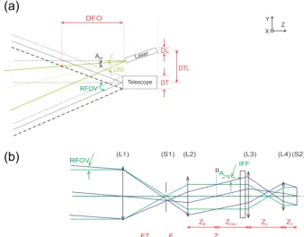
Figure 1. (a)The laser telescope geometry of a biaxial lidar system with a laser tiltAtiltand distance of full overlap DFO. RFOV and LBD
are the receiver’s field of view and laser beam divergence respectively (half angles). Due to the small angle approximation, the errors are negligible when defining the laser beam diameter (DL), as if the laser was not tilted, and the distance between the laser telescope central axes (DTL) at the back of the laser and telescope.(b)The optical setup of a lidar receiving unit with a telescope (L1), field of view diaphragm LBD (S1), collimating lens (L2), interference filter and objective lens (L3) and an eyepiece lens (L4). Rays collected from on-axis (green lines) and off-axis points (blue lines) with the maximum incident angle at the telescope (RFOV), which is limited by the FOVD, reaches the IFF surface with a free aperture diameter ofDobj, located at distanceZ1from L2 under an incident angleAmax. S2 is the surface of the PMT
with diameterDPMT.
This study focuses on the extension of the paraxial ap-proximation down to the detector, revealing all the possible constraints of a lidar setup, since DFO depends on the over-all optical path of the detected backscattered radiation. The distance of full overlap, as presented in this work, depends on the entire geometry considering all the parts of the lidar as one optical system. The analysis in this study highlights the need to take into consideration the acceptance angle of the interference filter when designing an optimized lidar sys-tem and the possible limitations that this imposes. The cor-responding geometrical formulation is presented in Sect. 2, describing the basic characteristics (focal lengths, distances and diameters) of all the optical components, compromised with the EARLINET QA standards. The derived formulation also includes the characteristics of an eyepiece lens, which has to be used in a lidar setup in order to form an image of the entrance pupil on the surface of the photodetector so as to spread the collected light uniformly over this image. The results of ray-tracing simulations with respect to lidar design and alignment according to geometrical formulation are pre-sented in Sect. 3.
The entire set of equations has been integrated in a Microsoft Excel worksheet through Visual Basic for Appli-cations (VBA) code and distributed with supplementary doc-umentation to the members of EARLINET network (http: //www.meteo.physik.uni-muenchen.de/~stlidar/earlinet_ asos/raytracing/Basic_design/basic_lidar_design.html), but can also be widely available upon request from the author ([email protected]). The aforementioned worksheet cannot substitute advanced optical design software. However, it may be complementary to the preliminary design of a system, can be used as a quick checkup tool for an existing lidar system or even used as a learning tool to familiarize a system with an optical lidar setup.
2 Lidar optical setup and limitations
diame-ter of 5 mm, an overall magnification of the optical system of 0.0166 is necessary. On the other hand, the angular magnifi-cation is increased by 60, which means that 1.25 mrad field of view of the receiver setup (i.e., determined by telescope with focal length 600 mm and a field stop with diameter 1.5 mm), is magnified to about 75 mrad (∼4.3◦).
For single but more particularly for multiwavelength sys-tems, the wavelength separation unit is not capable of accept-ing such a divergent received light beam, since (a) it would soon be too wide for 1 or 2 inch optical elements, and (b) the transmission of interference filters is very sensitive to the in-cidence angle. Therefore, the magnification of the receiver optics is split in two parts, i.e., the telescope with a collima-tion lens and another objective with an eyepiece, with a low divergent light path (parallel received light beam) in between (Fig. 1b). The inclination of the parallel beam is determined by the laser beam divergence, the laser telescope axis dis-tance, the tilt of the laser beam with respect to the telescope axis, determining the field of incidence angles into the tele-scope, and the magnification of the telescope together with the collimating lens.
The limitations for this inclination of the received rays are the following: the field of view of the telescope should be as small as possible in order to reduce the background light collected from the sky; the laser beam diameter and its di-vergence must both be small enough to fit through the 1 inch optics for all necessary beam splitters; the inclination must be less than the maximum acceptance angles of the interfer-ence filters.
2.1 Lidar optical layout
The setup of a biaxial lidar system is schematically given in Fig. 1. The laser telescope geometry is demonstrated in the upper part (Fig. 1a) while the optical setup of the lidar receiv-ing unit behind the telescope, is presented in the lower part (Fig. 1b). The abbreviations used in this study in order to de-scribe the lidar parameters are summarized in the Appendix as a list of abbreviations.
The modeling of a transmitted laser beam in the atmo-sphere has been approximated by a truncated cone of an ide-ally circularly shaped beam with initial diameter DL and di-vergence LBD (half angle). The DL and LBD values pro-vided by the manufacturers usually correspond to the 86.5 % (2σ )of the Gaussian beam energy. In lidar optical systems, the highest possible of the laser energy is needed and, to ac-count for a Gaussian laser beam containing the 98.9 % (3σ ) of the beam energy, both DL and LBD have to be reduced by a factor of 0.5. The laser beam interacts with the atmospheric constituents (aerosols and molecules) and the backscattered light is collected by a telescope with a focal length FT and clear aperture DT. The distance between the transmitter and receiver central axes is DTL (Fig. 1a). The diaphragm is usu-ally a circular iris, with diameter DFS centered on the
op-tical axis, and mounted on telescope’s focal plane. The
fo-cal length of the telescope and the diaphragm FOVD deter-mine the RFOV (half angle) of the receiver setup, according to RFOV= DFS
2×FT.
For simplicity, all the optical components of the sys-tem (telescope and lenses) are presented as thin lenses in Fig. 1b. In addition to the paraxial approximation assump-tion, namely that rays are not too distant from the system axis and their angles with respect to that axis are small, it also implies that aberration effects are not considered.
Regardless of the origin point of the incoming rays, any rays incident at the telescope with angles higher than RFOV will not pass through the diaphragm (FOVD; S1). Such a scenario is demonstrated in Fig. 1b where two extreme lines are shown: a green line representing rays parallel to the axis passes through the center of the field stop and normally im-pinges on the interference filter and a blue line which rep-resents extreme rays grazes the edge of the field stop at the maximum angle with respect to the normal to the interference filter (Fig. 1b). The entire range of angles of rays passing through any point of the telescope aperture and any point of the field stop must be limited by the collimating lens (L2; col-limator) with diameterDcol and focal lengthFcol, mounted
at distanceFcolbehind the field stop. The collimation of the
rays is mandatory due to the limited acceptance anglesAmaxIFF. of the IFFs (see Appendix). The collimating lens (L2) pro-duces an intermediate image (II) of the entrance pupil, at a distance ZII behind that lens. More precisely, the
inter-mediate image is formed at the so called eye-relief plane, where rays with different inclinations passing through the same points of the aperture cross each other. In the optical setup presented here, this plane appears twice; firstly behind the collimator and secondly behind the eyepiece. Regarding the first position, in case an optical detection device (e.g., PMT) is mounted there, it will collect all the power carried by rays reaching the aperture within the field of view, provided that its diameter is larger (or at least equal) than the image of the aperture formed by the collimating lens on that plane. This requires detection devices of large aperture (e.g., 1–2 inches) and consequently of high cost. However, by using an additional optical system assembled from an objective (L3) and an eyepiece lens (L4), this image will be formed again behind the eyepiece to a lower diameter. An objective lens (L3) with focal lengthFobjand diameterDobjis located just
behind the IFF and at a distanceZ1behind the collimator. An
eyepiece lens (L4) with focal lengthFeyeand diameterDeye
is placed at a distance ofZ2=Fobj+Feyebehind the
objec-tive lens. The focal length of the objecobjec-tive lens must not be shorter than three times its diameter, since for lowFobjvalues
of a simple, planoconvex or biconvex lens, the final image of the telescope aperture on the photomultiplier (PMT) may be affected by aberration effects. The PMT (S2) with diameter DPMTis located at distanceZ3behind the eyepiece lens and
and should be accurately mounted on the optical path of the collected backscattered light in order to achieve an optimum imaging (e.g., avoiding vignetting effects, keeping the con-dition thatAmax≤AmaxIFF)of the telescope’s aperture onto the
detector’s effective surface.
In principle, the system presented in Fig. 1b spreads uni-formly over the image of the entrance aperture formed on the photodetector surface the light coming from the illuminated parts of the atmosphere within the system field of view. The effective diameter of the photomultiplier is maximum 8 mm for Hamamatsu PMTs R7400 series (Hamamatsu Photonics, 2006). However, the useful diameter of the PMT is about 5 mm, including mounting and adjustment tolerances.
For ranges above the DFO, the laser beam stays entirely inside the telescope’s full field of view. For those ranges, any ray coming from a point in the illuminated volume and reach-ing the telescope aperture will pass through the field stop di-aphragm.
2.2 Description through paraxial approximation The parameter of RFOV is chosen as the coupling link be-tween the laser telescope part and the detection optics, which are located after the telescope focus. This choice can be ex-plained, since on one side the given telescope and laser geo-metrical characteristics determine the DFO, and on the other side towards the PMT, all rays entering the field stop have to be collected by the PMT.
As also demonstrated from Stelmaszczyk et al. (2005) from Fig. 1a we have the following:
DFO= 2×DTL+DT+DL
2×(RFOV−LBD+Atilt)
. (1)
In the case that a laser beam expander with an expansion factor of EX is used in the emission part of a biaxial lidar configuration, the initial laser diameter increases and the cor-responding laser beam divergence decreases, by a factor of EX. Thus, the effective laser parameters (DL and LBD) af-ter the expansion will become respectively, DL×EX and LBD×EX−1, in all formulas. The above are approximations and hold true for ideal optical components, since in general, commercial laser beam expanders demonstrate different effi-ciencies regarding the expansion of the laser beam diameter and the reduction of the laser beam divergence.
The dominator of Eq. (1) must be positive (i.e., RFOV−
LBD+Atilt≥0)in order to have DFO≥ 0. This, together
with the condition that Atilt+LBD≤ RFOV leads to the
basic principle for lidar applications that the receiver’s field of view cannot be smaller than the laser beam diver-gence (i.e., RFOV≥LBD). In the case that the condition Atilt+LBD≤RFOV is not fulfilled, even if the full overlap is
reached in some range, the laser beam will eventually exit the full field of view zone in the far range. With paraxial optics
and small angle approximation, we can extract from Fig. 1b the following relation:
RFOV= DFS
2×FT = Fcol
FT ×Amax, (2)
whereAmaxis the maximum incidence angle on the
inter-ference filter of rays passing through the field stop. This an-gle should be less than or equal to the maximum acceptance angle of the interference filter:
Amax≤AmaxIFF . (3)
The main goal when designing a lidar system for aerosol re-search in the lower to middle troposphere is to make the DFO as short as possible while keeping (a) the incidence angle of the rays on the interference filter surface less than its accep-tance angle (i.e.,Amax≤AmaxIFF.)and (b) the diameters of the
lenses within reasonable values. For the use of a small band-width IFF with smallAmaxIFF it is necessary to keep the RFOV small or to increase the ratio Fcol
FT. In biaxial lidar systems
the RFOV is determined by the parameters of the receiver setup (FT andDFS), and the higher the RFOV, the lower
the DFO ranges that may be achieved (Eq. 1). In addition, by increasing theDFSthe RFOV increases (Eq. 2) and the
DFO decreases but the SNR becomes lower, especially dur-ing daytime conditions when the detected lidar signal is con-taminated with more light from the sky background. More-over, high RFOV values tend to increase the diameters of the lenses in the receiving optical setup.
With AIFF=Amax and for any Atilt from Fig. 1b and
Eqs. (1) and (2) we get
DFO= 2×DTL+DT+DL
2×Fcol
FT ×Amax−LBD+Atilt
. (4)
The ratio Fcol
FT is limited by the diameters ofDcoland DT
(compare Fig. 1b) by
Dcol≥DT×
Fcol
FT +2×RFOV×(FT+Fcol) . (5) Consequently,
Dcol
2 −RFOV×FT
Fcol
≥
DT
2 +RFOV×FT
FT . (6)
Additional constraints are the limited diameters of the lenses, filters and beam splitters in combination with the di-ameter and the focal lengths of the telescope and the collima-tor (i.e., FT andFcol), as well as the distanceZ1which needs
lidar systems. Note, that the diameterDcolof the optical parts
is limited by their rising cost with diameter and decreasing availability. The extreme rays in Fig. 1b must pass through all the optics, which results in Eq. (6), expressed here for the minimum and maximum focal length of the telescope with given RFOV.
FTmax/min=0.5×
D
col
2×RFOV−Fcol
±
s
0.25×
Fcol−
Dcol
2×RFOV
2
− Fcol×DT
2×RFOV (7)
All these parameters must be balanced for optimum lidar performance and for a specific scientific objective. The fol-lowing system of equations (Eq. 8) is derived with paraxial approximation (Fig. 1b). The first one is given by definition (Fig. 1b), the second one gives the plane where the image of the entrance pupil by the collimating lens is formed, and the third one gives the minimum diameter that the objective lens must have in order to let all the rays within the field of view pass:
Z1=Zobj+ZII
ZII=
RFOV Amax
×(Fcol+FT)
Dobj
2 =
DT×Fcol
FT
2 +Amax×Zobj
yields
−→ Z1=
1 2×Amax
×
Dobj−DT×
Fcol
FT +2×RFOV×(Fcol+FT)
. (8)
Furthermore, in the ZII expression that appears in the
block of Eq. (8), the term RFOVA
max has been substituted for Fcol
FT.
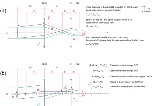
Following Figs. 1b and 2a, the diameter of the intermediate image (DII)formed on the eye-relief plane between the
col-limator and the objective lens, and the diameter of the objec-tive lens(Dobj)just behind the IFF are equal to
DII=
DT
FT ×Fcol (9)
Dobj=DII+2×Amax×Zobj. (10)
The rays collected by the IFF and the objective lens (L3 in Fig. 1b) are guided through the eyepiece lens (L4 in Fig. 1b), creating the final image of the entrance pupil at a distance Z3 behind the last surface of the eyepiece lens. More
pre-cisely, the intermediate image of the telescope aperture (with diameterDII)is formed initially at distanceZobjbefore the
objective lens (L3; Figs. 1b and 2). In the setup presented in Fig. 2, the intermediate image is now the object with diam-eter DIIthat has to be projected on the surface of the
pho-todetector (S2) through the system of two lenses. The first
lens of this system is an objective lens (L3) with focal length Fobj, and the second one is an eyepiece lens (L4) with focal
lengthFeye. In this setup, the back focal plane of the objective
and the front focal plane of the eyepiece coincide; i.e., the separation between the objective and the eyepiece is equal toZ2=Fobj+FeyeThe total magnification of that lens
sys-tem isM3,4=FFeye
obj. Therefore, the final image of the object (DII)projected on (S2) would have the following diameter
(Fig. 2a):
DPMT≥M3,4×DII→Feye≤
DPMT
DII
×Fobj. (11)
From the similarity of the triangles shown in Fig. 2b we find thatR3= FRobj1 ×Feye, whereR1 is the diameter of an
object produced by of off axis rays on the intermediate plane (Fig. 2b). The free aperture of the lens (L4) in order to collect both off and on-axis points ofDIIhas to beDeye(Fig. 2b):
Deye=2× "
Amax×Fobj+
DII
2 −Amax× Zobj−Fobj
Fobj ×Feye #
. (12) Considering as object the image of the aperture by L2, which is at distance Zobj of L3, the afocal system of the
lenses L3 and L4 will project it, at a distanceZ3behind L4.
This distance is
Z3=Feye×
"
1−Feye
× Zobj−Fobj
Fobj2
#
. (13)
PMTs and APDs suffer from a non-uniform spatial re-sponse of their effective surface, which may cause artifacts to lidar signals during its transduction into electrical signal. Simeonov et al. (1999) revealed that the normalized spatial uniformity on the active area of the detector varies from 0.2 up to almost three times the average value, defined for the central part of the detector. In order to avoid lidar signal devi-ations due to the spatial inhomogeneity PMT sensitivity, the detector must be placed at an image of the telescopes aper-ture. At this place (distanceZ3behind the eyepiece lens; L4),
Figure 2.Panels(a)and(b)are essentially the same. However, to help the understanding of geometric calculations,(a)demonstrates the optical path of the on-axis (green line) and off-axis (blue line) points, the first intermediate image (II) of the telescope aperture with diameter DIIformed at distanceZobjbefore the objective lens (L3) and(b)the optical path of the on-axis (green line) and off-axis (blue line) points,
of an object (with diameterR1)produced by off-axis points on the intermediate plane. Through the objective lens (L3) with focal length
Fobjand an eyepiece lens (L4) with focal lengthFeyethe intermediate image is formed again on the surface of the photodetector (S2), at
a distanceZ3behind the eyepiece lens. For reasons of simplicity the IFF is not included in this figure. The focal planes of each lens are
denoted with vertical red lines on the principal axis.
For boundary layer measurements a low DFO height is re-quired (see Fig. 1a), thus leading to higher values of Amax
(Eq. 4), larger IFF bandwidth, lower sky background sup-pression and finally lower SNR of the system.
Tilting the laser by an angleAtiltwith respect to the
tele-scope axis (Fig. 1a), with the constraint thatAtilt≤RFOV−
LBD,allows a decrease of the RFOV with constant DFO or a decrease of the DFO with constant RFOV (Stelmaszczyk et al., 2005). The optimumAtiltis either the one that minimizes
the RFOV or the DFO respectively, and for both aforemen-tioned cases becomes equal to
Aopttilt =RFOV−LBD. (14) More clearly, for the former scenario
Aopttilt=2×DTL+DT+DL
4×DFO , (15)
and withAopttilt according to Eq. (2)
Amax=
FT Fcol
×
2×DTL+DT+DL
4×DFO +LBD
(16) .
The IFF allows for acceptable transmission of the backscattered rays with incident angles lower thanAmaxIFF (see Appendix). The smaller the filter bandwidth, the smaller theAmaxIFF (a filter with bandwidth BW=0.5 nm, leading to AmaxIFF =2.9◦). The extreme incident angles in the telescope (RFOV)and at the IFF (Amax)increase with decreasing DFO
Figure 3.The variability of the maximum angle of incident rays on the IFF (Amax)for different DFO values, without laser tilt (Atilt=
00; black line) and with optimum laser tilt (Aopttilt.=095 mrad; red line). The blue horizontal dashed lines correspond to the maximum acceptance angles (2.9 and 1.15◦) of two IFFs with bandwidths of 0.5 and 0.15 nm respectively (see Appendix).
In Fig. 3 the variation of the maximum angle of incident rays on the IFF (Amax)for different DFO values is presented,
regarding zero degrees and optimum laser tilt (Aopttilt), accord-ing to Eqs. (4) and (16). The values used for the calculations (e.g., FTFcolDTLDTDL)are provided in Sect. 3. The
max-imum angle of incident rays (Amax)on the IFF is decreased
by about 40 % (from 1.96 to 1.15◦) with an optimum laser
tilt for the same DFO (182.11 m). The two blue lines indi-cate theAmaxIFF angles for two IFFs with BW 0.5 and 0.15 nm respectively (see Appendix).
3 Evaluation of paraxial approximation with ray-tracing simulations
For evaluating the formulation presented in this study, ray-tracing simulations with ZEMAX software (www.zemax. com) have been performed. Considering that, unlike ZE-MAX, various aberration effects are not taken into account with thin lens approximation, in this section it is investigated how close the calculations are in reality when derived in com-parison with real ray-tracing simulations.
The geometrical properties of the simulated lidar system used as input parameters in paraxial approximation lead to a DFO =257 m. More precisely, a laser with initial param-eters DL=8 mm and LBD =0.8 mrad was considered and expanded by an ideal laser beam expansion unit(EX= ×4). The expansion unit finally results in an emitted laser beam with a diameter of 32 mm and divergence LBD =0.2 mrad. Moreover, the laser beam is considered to be tilted towards the telescope central axis with an angle of Atilt=0.4 mrad.
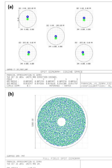
Figure 4.Spot diagrams of far- (green; 10 000 m) and near- (blue; 257 m) range rays on the(a)front surface of the IFF from five differ-ent positions within the receiver field of view, and(b)PMT detector with 5 mm effective diameter (black circle).
The laser light scattered in the atmosphere is collected by an ideal telescope with DT=300 mm and FT=600 mm, guided through a circular field stop (DFS=1.5 mm) to the
collima-tor. The distanceZ1has to be as high as possible to mount
all the needed optical elements (i.e., beam splitters), always keepingAmaxlower thanAmaxIFF.. Considering a receiving
sys-tem with RFOV=1.25 mrad, effectiveDobj.=23.5 mm and a reasonably lowAmaxvalue (Amax=1.15◦),a distance of
Z1=160 mm, is estimated through Eq. (8). Moreover, for
these values Eq. (2) implies that the focal length of the colli-mator should beFcol=37.36 mm.
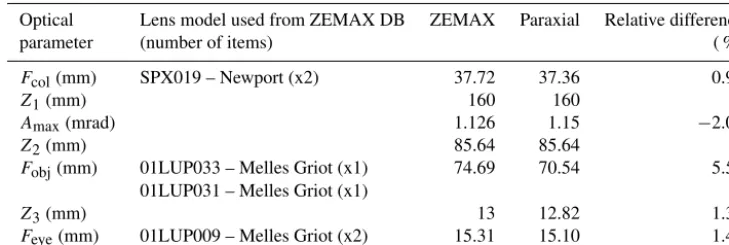
Table 1.The optical parameters (distances and focal lengths) estimated with paraxial approximation and simulated by ZEMAX, along with their relative differences.
Optical Lens model used from ZEMAX DB ZEMAX Paraxial Relative difference
parameter (number of items) ( %)
Fcol(mm) SPX019 – Newport (x2) 37.72 37.36 0.95
Z1(mm) 160 160 0
Amax(mrad) 1.126 1.15 −2.08
Z2(mm) 85.64 85.64 0
Fobj(mm) 01LUP033 – Melles Griot (x1) 74.69 70.54 5.56
01LUP031 – Melles Griot (x1)
Z3(mm) 13 12.82 1.38
Feye(mm) 01LUP009 – Melles Griot (x2) 15.31 15.10 1.42
backscattering from the laser beam was simulated by a disk of source rays, which was placed at distances of 257 m and 10 000 m from the telescope. Assuming that the telescope and the laser beam are at the same level (Fig. 1b), then the initial distance between their central axis was considered to be DTL=180 mm. However, as the laser beam propagates in the atmosphere with a tilting angle of 0.4 mard, the distance between the laser beam and telescope central axis decreases with a constant rate of Atilt. For each distance,
the size of the laser disk was calculated from the LBD. Regarding the optical components mounted after the field stop, we used lenses available from the ZEMAX database, with parameters (i.e., effective focal length and diameter) similar to the ones revealed from the paraxial approximation calculations. More precisely, x2 Newport (model SPX019) lenses were used as collimator (effective Fcol=37.72 mm
andDcol=25.40 mm), x2 Melles Griot (models 01LUP033
and 01LUP031) were used as an objective (effective Fobj=74.69 and Dobj=25.00 mm) and x2 Melles Griot
(model 01LUP009) lenses were used as an eyepiece lens (effective Feye=15.31 and Deye=12.50 mm; Table 1). In
ZEMAX we set the distance between the collimator and the IFF at exactly 160 mm (Z1), the eyepiece at 85.64 mm after
the IFF (Z2), while the distance between the eyepiece and
PMT was at 13 mm. The value of distanceZ3was not kept
constant in the ZEMAX simulation as it was estimated from the paraxial calculations. Instead, this distance was slightly increased up to some millimeters in order to sufficiently image the telescope aperture on the PMT (DPMT=5 mm),
without any truncation of the rays. Please note here that, in the case of real simulations with ZEMAX, the lenses cease to be ideal thin lenses. The distances, namely Z1,
Z2 andZ3, are measured from the points on the principal
axis of the last surface of each lens up to the first surface of the next optical component. For example, the measured distance Z1 refers to the distance between the last surface
of the collimator up to the first surface of the IFF filter, located on the principal axis. In Fig. 4 the spot diagrams of rays from far (green spots; 10 000 m) and near range (blue spots; 257 m) are demonstrated. The five field points
selected so as to make an object height with radius equal to LBDx Z+DL
2 , where Z is the atmospheric distance from
the lidar. The central field point is located at the center of the disk, with coordinates(xC, yC)=(0,DTL−Z×Atilt),
with respect to the Cartesian system shown in Fig. 1a, while the remaining four are selected to be on the perimeter of this disk with coordinates (xR, yR)= (−Z×LBD, yC), (xLyL)=(Z×LBD, yC) , (xU, yU)= (0, yC+Z×LBD) , (xD, yD)=(0, yC−Z×LBD). The spot diagrams in Fig. 4a are in cosine space, demonstrating the angle with which each field point of far- and near-range rays falls on the first surface of the IFF filter. The maximum field incident angle on the IFF was found to be equal to 0.0196 mrad. The full field spot diagram demonstrated in Fig. 4b refers to the surface of the PMT. As can be seen in Fig. 4b a homogeneous distribution of far- and near-range rays on PMT surface have been achieved, covering the same area. The spot diameter was found to be 4.6 mm, within the 5 mm diameter of effective detector aperture, revealing an overall sufficient imaging of far- and near-range rays on the detector.
The relative differences between the calculated parame-ters from paraxial approximation and the simulations with ZEMAX are demonstrated in Table 1, and the slight dis-crepancies are attributed to the following reasons: (a) the slightly different parameters of lenses used from ZEMAX database compared to those used as input (Fcol)or estimated
(FobjFeye)with the paraxial approximation formulation and
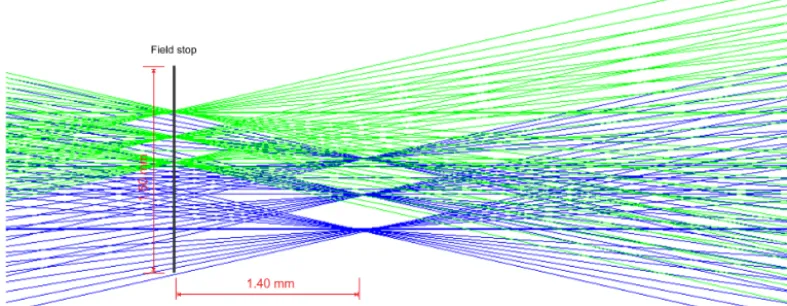
Figure 5.ZEMAX simulations regarding the focal plane of the telescope where the field stop (DFS=15 mm) is placed. The focal plane is
where parallel rays will intersect after passing through the telescope. Rays arriving at the telescope from near points will intersect behind the focal plane. Where they finally intersect depends on how near the origin point is. Rays originating from points at 257 m from the lidar (blue lines) intersect at 1.4 mm behind the focal plane of the telescope. As the points are taken farther away, the intersection point will tend to approach the focal plane, eventually being virtually on the focal plane for long enough distances (i.e., the points from 10 000 m considered here with green lines).
long enough distances (i.e., the points from 10 000 m consid-ered here with green lines). From the paraxial formula relat-ing object and image positions, a simple calculation shows that, for a thin lens of 600 mm focal length, the image of a point at 10 000 m from the lens will be at 600.04 mm from the lens plane, while the image of a point at 257 m will be at 601.40 mm, the difference being 1.36 mm, very close to the 1.40 mm revealed by ZEMAX simulations (Fig. 5). Thus, the telescope processes the rays according to the paraxial optics laws (or at least to a good degree of approximation), so the considered rays satisfy the paraxial conditions.
4 Summary and conclusions
Based on thin lens approximation formulas, a set of equa-tions is derived, describing the optical design of a typical EARLINET lidar system. The limitations of a lidar optical setup are revealed through geometric optics, from the emitted laser beam to the projection of the entrance pupil on the pho-tomultiplier. The main lidar issue studied here concerns the distance of full overlap and how this depends on the entire geometry which describes the optical path in the detection unit of a lidar system, not only on the laser telescope geom-etry. The usage of IFF with small bandwidth for background suppression is limited by their small acceptance angle, espe-cially if the alignment uncertainties of the mechanical setup of the lidar optics are taken into account. The evaluation of the paraxial approximation formulation has been performed with ZEMAX ray-tracing simulations, showing an overall good performance with a relative difference (between ZE-MAX and paraxial approximation) of the order of 5 % (see Table 1) and a negligible impact on the system performance.
These differences are mainly attributed to the inability of thin lens formulations to better model the refraction of the off-axis rays. The described formulation cannot substitute an advanced optical design software, since 3-D ray-tracing sim-ulations of realistic lidar systems are required to reveal the necessity of using the highest-quality optical parts mounted with the highest possible accuracy.
Appendix A
The center wavelength λo of an interference filter (IFF) is shifted toλswith an incident angleAIFFaccording to
λs
λo
=
s
1−
n
o ne
×sin(AIFF)
2
, (A1)
with the effective refractive index of the filter ne and
the refractive index of the environment no. The shift is to smaller wavelengths with increasing AIFF, and larger ne.
Examples for IFF are a Barr filter with 0.5 nm bandwidth (BWFWHM)at 532 nm,ne=1.99 and a temperature
coef-ficient of 0.0021 nm◦C−1, as well as an Andover filter with
BW=0.15 nm at 532 nm,ne=1.45 and temperature
coeffi-cient 0.016 nm◦C−1. The incident anglesAIFFare limited by
the maximum allowed wavelength shift for acceptable trans-mission, which have been set to 0.7×BW
2 ,i.e., about 0.18 nm
(Barr) and 0.05 nm (Andover). This results in AmaxIFF. of 2.9 and 1.14◦for Barr and Andover filters respectively.
Appendix B: A list of the abbreviations that are used for describing the lidar parameters, along with their
meaning Object space
DFO The distance of full overlap of the lidar system DTL The distance between telescope and laser central axis DT The clear aperture of the telescope
DL The diameter of the laser beam FT The focal length of the telescope RFOV The receiver field of view (half angle) LBD The laser beam divergence (half angle)
Atilt The inclination angle of the laser beam axis relative to the telescope axis
Image space
DFS The diameter of the field stop
FOVD The field of view diaphragm
Fcol The focal length of the collimating lens
Dcol The diameter of the collimating lens
AIFF The incidence angle of the rays on the interference filter
Amax. The maximum incidence angle on the interference filter of rays passing through the field stop AmaxIFF. The maximum acceptance angle of the interference filter
Z1 The distance between the collimator and the objective lens
ZII The distance between the collimator and the plane of intermediate image
DII The diameter of the intermediate image
Zobj The distance between the plane of intermediate image and the objective lens
Fobj The focal length of the objective lens
Dobj The diameter of the objective lens
Z2 The distance between the objective and the eyepiece lens
Z3 The distance between the eyepiece lens and the detector
Feye The focal length of the eyepiece lens
Deye The diameter of the eyepiece lens
Competing interests. The authors declare that they have no conflict of interest.
Special issue statement. This article is part of the special issue “EARLINET, the European Aerosol Research Lidar Network”. It is not associated with a conference.
Acknowledgements. I would like to thank Volker Freudenthaler for the helpful discussions, ideas and useful comments.
The publication was supported by the European Union Seventh Framework Programme (FP7-REGPOT-2012-2013-1) in the framework of the project BEYOND, under grant agreement no. 316210 (BEYOND-Building Capacity for a Center of Excellence for EO-based monitoring of Natural Disasters).
Edited by: Albert Ansmann
Reviewed by: two anonymous referees
References
Abramochkin, A. I. and Tikhomirov, A. A.: Optimization of a lidar receiving system 2, Spatial filters, Atmos. Ocean. Opt. 12, 331– 342, 1999.
Amiridis, V., Melas, D., Balis, D. S., Papayannis, A., Founda, D., Katragkou, E., Giannakaki, E., Mamouri, R. E., Gerasopoulos, E., and Zerefos, C.: Aerosol Lidar observations and model calcu-lations of the Planetary Boundary Layer evolution over Greece, during the March 2006 Total Solar Eclipse, Atmos. Chem. Phys., 7, 6181–6189, https://doi.org/10.5194/acp-7-6181-2007, 2007. Ansmann, A., Riebesell, M., and Weitkamp, C.: Measurement of
atmospheric aerosol extinction profiles with a Raman lidar, Opt. Lett., 15, 746–748, https://doi.org/10.1364/OL.15.000746, 1990. Ansmann, A., Wandinger, U., Riebesell, M., Weitkamp, C., and Michaelis, W.: Independent measurement of extinction and backscatter profiles in cirrus clouds by using a combined Raman elastic-backscatter lidar, Appl. Opt., 31, 7113–7131, https://doi.org/10.1364/AO.31.007113, 1992.
Baars, H., Ansmann, A., Engelmann, R., and Althausen, D.: Con-tinuous monitoring of the boundary-layer top with lidar, Atmos. Chem. Phys., 8, 7281–7296, https://doi.org/10.5194/acp-8-7281-2008, 2008.
Belegante, L., Bravo-Aranda, J. A., Freudenthaler, V., Nicolae, D., Nemuc, A., Alados-Arboledas, L., Amodeo, A., Pappalardo, G., D’Amico, G., Engelmann, R., Baars, H., Wandinger, U., Pa-payannis, A., Kokkalis, P., and Pereira, S. N.: Experimental as-sessment of the lidar polarizing sensitivity, Atmos. Meas. Tech. Discuss., https://doi.org/10.5194/amt-2015-337, in review, 2016. Bösenberg, J.: Study on retrieval algorithms for a backscatter li-dar, Final report, Max-Plank- Inst. Für Meteorol., Hamburg, Ger-many, MPI-Rep. 226, 1997.
Bravo-Aranda, J. A., Belegante, L., Freudenthaler, V., Alados-Arboledas, L., Nicolae, D., Granados-Muñoz, M. J., Guerrero-Rascado, J. L., Amodeo, A., D’Amico, G., Engelmann, R., Pap-palardo, G., Kokkalis, P., Mamouri, R., Papayannis, A., Navas-Guzmán, F., Olmo, F. J., Wandinger, U., Amato, F., and Haeffe-lin, M.: Assessment of lidar depolarization uncertainty by means
of a polarimetric lidar simulator, Atmos. Meas. Tech., 9, 4935– 4953, https://doi.org/10.5194/amt-9-4935-2016, 2016.
Chourdakis, G., Papayannis, A., and Porteneuve, J.: Analysis of the receiver response for a noncoaxial lidar system with fiber-optic output, Appl. Opt., 41, 2715–2723, 2002.
Comeron, A., Sicard, M., Kumar, D., and Rocadenbosch, F.: Use of a field lens for improving the overlap function of a lidar system employing an optical fiber in the receiver assembly, Appl. Opt., 50, 5538–5544, 2011.
Dho, S. W., Park, Y. J., and Kong, H. J.: Experimental deter-mination of a geometric form factor in a lidar equation for an inhomogeneous atmosphere, Appl. Opt., 36, 6009–6010, https://doi.org/10.1364/AO.36.006009, 1997.
Eloranta, E. W.: Practical model for the calculation of mul-tiply scattered lidar returns, Appl. Opt., 37, 2464–2472, https://doi.org/10.1364/AO.37.002464, 1998.
Engelmann, R., Kanitz, T., Baars, H., Heese, B., Althausen, D., Skupin, A., Wandinger, U., Komppula, M., Stachlewska, I. S., Amiridis, V., Marinou, E., Mattis, I., Linné, H., and Ansmann, A.: The automated multiwavelength Raman polarization and water-vapor lidar PollyXT: the neXT generation, Atmos. Meas. Tech., 9, 1767–1784, https://doi.org/10.5194/amt-9-1767-2016, 2016.
Fernald, F. G., Herman, B. M., and Reagan, J. A.: Determination of Aerosol Height Distribution by Lidar, J. Appl. Meteorol., 11, 482–489, 1972.
Freudenthaler, V: Optimized background suppression in near field lidar telescopes, in: Proceedings 5 of the 6th International Sym-posium on Tropospheric Profiling: Needs and Technologies (ISTP 2003), edited by: Wandinger, U., Engelmann, R., and Schmieder, K., Institute for Tropospheric Research, 243–245, 2003.
Freudenthaler, V.: Effects of spatially inhomogeneous photomulti-plier sensitivity on LIDAR signals and remedies, in: Proceedings of the 22nd International Laser Radar Conference (ILRC 2004) held 12–16 July 2004 in Matera, Italy, edited by: Pappalardo, G. and Amodeo, A., European Space Agency, Paris, 37 pp., ESA SP-561, 2004.
Freudenthaler, V.: The telecover test: a quality assurance tool for the optical part of a lidar system, in: Reviewed and Revised Papers Presented at the 24th International Laser Radar Confer-ence, Boulder, Colorado, USA, 23–27 June 2008, Boulder, Col-orado, USA, presentation: S01P-30, available at: http://epub.ub. uni-muenchen.de/12958/ (last access: 8 July 2016), 2008. Freudenthaler, V.: About the effects of polarising optics on lidar
signals and the190 calibration, Atmos. Meas. Tech., 9, 4181– 4255, https://doi.org/10.5194/amt-9-4181-2016, 2016.
Freudenthaler, V., Esselborn, M., Wiegner, M., Heese, B., Tesche, M., Ansmann, A., Müller, D., Althausen, D., Wirth, M., Fix, A., Ehret, G., Knippertz, P., Toledano, C., Gasteiger, J., Garham-mer, M., and Seefeldner, M.: Depolarization ratio profiling at several wavelengths in pure Saharan dust during SAMUM 2006, Tellus B, 61, 165–179, https://doi.org/10.1111/j.1600-0889.2008.00396.x, 2009.
Haarig, M., Engelmann, R., Ansmann, A., Veselovskii, I., White-man, D. N., and Althausen, D.: 1064 nm rotational Raman lidar for particle extinction and lidar-ratio profiling: cirrus case study, Atmos. Meas. Tech., 9, 4269–4278, https://doi.org/10.5194/amt-9-4269-2016, 2016.
Halldórsson, T. and Langerholc, J.: Geometrical form fac-tors for the lidar function, Appl. Opt., 17, 240–244, https://doi.org/10.1364/AO.17.000240, 1978.
Hamamatsu Photonics: Photomultiplier tubes Basics and Applica-tions, 2 Edn., 1–305, 2006.
Iarlori, M., Madonna, F., Rizi, V., Trickl, T., and Amodeo, A.: Ef-fective resolution concepts for lidar observations, Atmos. Meas. Tech., 8, 5157–5176, https://doi.org/10.5194/amt-8-5157-2015, 2015.
Jenness, J. R., Lysak, D. B., and Philbrick, C. R.: Design of a li-dar receiver with fiber-optic output, Appl. Opt., 36, 4278–4284, 1997.
Klett, J. D.: Stable analytical inversion solution for processing lidar returns, Appl. Opt., 20, 211–220, https://doi.org/10.1364/AO.20.000211, 1981.
Matthias, V. and Bösenberg, J.: Aerosol climatology for the plan-etary boundary layer derived from regular lidar measurements, Atmos. Res., 63, 221–245, 2002.
Matthias, V., Balis, D., Bösenberg, J., Eixmann, R., Iarlori, M., Komguem, L., Mattis, I., Papayannis, A., Pappalardo, G., Perrone, M. R., and Wang, X.: Vertical aerosol dis-tribution over Europe: Statistical analysis of Raman li-dar data from 10 European Aerosol Research Lili-dar Net-work (EARLINET) stations, J. Geophys. Res., 109, D18201, https://doi.org/10.1029/2004JD004638, 2004.
Mattis, I., Tesche, M., Grein, M., Freudenthaler, V., and Müller, D.: Systematic error of lidar profiles caused by a polarization-dependent receiver transmission: quantification and error correction scheme, Appl. Opt., 48, 2742–2751, https://doi.org/10.1364/AO.48.002742, 2009.
Müller, D., Wandinger, U., and Ansmann, A.: Microphysical parti-cle parameters from extinction and backscatter lidar data by in-version with regularization: theory, Appl. Opt., 38, 2346–2357, https://doi.org/10.1364/AO.38.002346, 1999.
Pappalardo, G., Amodeo, A., Apituley, A., Comeron, A., Freuden-thaler, V., Linné, H., Ansmann, A., Bösenberg, J., D’Amico, G., Mattis, I., Mona, L., Wandinger, U., Amiridis, V., Alados-Arboledas, L., Nicolae, D., and Wiegner, M.: EARLINET: to-wards an advanced sustainable European aerosol lidar network, Atmos. Meas. Tech., 7, 2389–2409, https://doi.org/10.5194/amt-7-2389-2014, 2014.
Sasano, Y., Shimizu, H., Takeuchi, N., and Okuda, M.: Ge-ometrical form factor in the laser radar equation: an experimental determination, Appl. Opt., 18, 3908–3910, https://doi.org/10.1364/AO.18.003908, 1979.
Sassen, K.: Polarization in Lidar, in Lidar, edited by: Weitkamp, D. C., 19–42, Springer New York, available at: http://link.springer. com/chapter/10.1007/0-387-25101-4_2 (last access: 29 March 2016), 2005.
Simeonov, V., Larcheveque, G., Quaglia, P., van den Bergh, H., and Calpini, B.: Influence of the photomultiplier tube spa-tial uniformity on lidar signals, Appl. Opt., 38, 5186–5190, https://doi.org/10.1364/AO.38.005186, 1999.
Stelmaszczyk, K., Dell’Aglio, M., Chudzy´nski, S., Stacewicz, T., and Wöste, L.: Analytical function for lidar geometrical com-pression form-factor calculations, Appl. Opt., 44, 1323–1331, 2005.
Tomine, K., Hirayama, C., Michimoto, K., and Takeuchi, N.: Exper-imental determination of the crossover function in the laser radar equation for days with a light mist, Appl. Opt., 28, 2194–2195, https://doi.org/10.1364/AO.28.002194, 1989.
Veselovskii, I., Kolgotin, A., Griaznov, V., Müller, D., Wandinger, U., and Whiteman, D. N.: Inversion with regularization for the retrieval of tropospheric aerosol parameters from mul-tiwavelength lidar sounding, Appl. Opt., 41, 3685–3699, https://doi.org/10.1364/AO.41.003685, 2002.
Veselovskii, I., Dubovik, O., Kolgotin, A., Lapyonok, T., Di Giro-lamo, P., Summa, D., Whiteman, D. N., Mishchenko, M., and Tanré, D.: Application of randomly oriented spheroids for re-trieval of dust particle parameters from multiwavelength li-dar measurements, J. Geophys. Res.-Atmos., 115, D21203, https://doi.org/10.1029/2010JD014139, 2010.
Veselovskii, I., Whiteman, D. N., Korenskiy, M., Suvorina, A., and Pérez-Ramírez, D.: Use of rotational Raman measure-ments in multiwavelength aerosol lidar for evaluation of parti-cle backscattering and extinction, Atmos. Meas. Tech., 8, 4111– 4122, https://doi.org/10.5194/amt-8-4111-2015, 2015.
Wandinger, U.: Multiple-scattering influence on extinction-and backscatter-coefficient measurements with Raman and high-spectral-resolution lidars, Appl. Opt., 37, 417–427, 1998. Wandinger, U.: Introduction to Lidar, in Lidar, edited by: Weitkamp,
D. C., 1–18, Springer New York, available at: http://link. springer.com/chapter/10.1007/0-387-25101-4_1 (last access: 8 July 2016), 2005.
Wandinger, U. and Ansmann, A.: Experimental determination of the lidar overlap profile with Raman lidar, Appl. Opt., 41, 511–514, https://doi.org/10.1364/AO.41.000511, 2002.