Fitting Models of Vulnerability to Toxicity with Generalized Linear Models

(1)

http://www.sciencepublishinggroup.com/j/ijdsa doi: 10.11648/j.ijdsa.20170305.13

ISSN: 2575-1883 (Print); ISSN: 2575-1891 (Online)

Fitting Models of Vulnerability to Toxicity with Generalized

Linear Models

Ganiyu Abayomi Dawodu

Statistics Department, College of Physical Sciences, Federal University of Agriculture, Abeokuta (FUNAAB), Nigeria

Email address:

[email protected]

To cite this article:

Ganiyu Abayomi Dawodu. Fitting Models of Vulnerability to Toxicity with Generalized Linear Models. International Journal of Data Science and Analysis. Vol. 3, No. 5, 2017, pp. 46-57. doi: 10.11648/j.ijdsa.20170305.13

Received: August 21, 2017; Accepted: September 15, 2017; Published: November 8, 2017

Abstract:

People are often exposed to toxic or hazardous (e.g. radioactive radon and lead) elements and rays, without even knowing so. Toxicity often results from an individual’s prolonged exposure to toxic substances. A thorough examination of some individuals’ blood or urine samples for the quantities of hazardous substances or elements, often gives a multivariate data (i.e. matrix of cases against elements) on toxicity. The pertinent response variable is often binary response (or count data) type and hence the Generalized Linear Models (GLM) of it can be fitted using our proposed techniques. This paper purports to identify models in GLM that can be used to study toxicity when it is ‘captured’ as count data or Binary Response Variables (BRV). An illustration of how the techniques work is done by using a sample of data on some artisans.

Keywords:

GLM, Exploratory Data Analysis (EDA), BRV, Count Data (CD), Toxicity, R

1. Introduction

Pollution happens in various ways; environmental and occupational exposures to pollutants are usually experienced by artisans [4]. Environmental pollution can sometimes be due to human inappropriate activities (e.g. the dumping of toxic waste in residential locations) or natural (e.g. the natural emission of radioactive radon in residential buildings (indoor radon)) [5] [6] [7]. In the former case, the activity can be easily stopped, whilst in the latter case, little or nothing can be done. With respect to occupational exposure; some measures can be put in place to usurp their effects on humans or, at least, reduce the effects to the barest minimum. It is because of occupational exposure that the technologists, and artisans, working in radioactive environments, are strongly advised to display the ‘symbol’ for radioactivity in a conspicuous location around their laboratories and workshops respectively and to always use protective gadgets and advise their patrons and customers to do the same. Accidental exposure is also possible, it may happen in a mineral mining field or at a nuclear energy station such as the one of Chernobyl and Fukushima [4]. When people are in a polluted environment, they are said to be exposed to dangerous (or toxic) substances (e.g. indoor radon, fungi spores, and lead). Hence toxicity, in an individual, often

results from his/her prolonged exposure to toxic substances. The individual will be ‘pronounced’ toxic, with respect to the toxic substance, if the estimated quantity of the substance found in the samples (e.g. blood or urine) from his/her body is higher than the quantity that can be tolerated by a human body (i.e. without associating any allied ailments). Upon a thorough examination of some individuals’ blood or urine samples for the quantities of ‘hazardous’ substances or elements, a multivariate data (i.e. matrix of cases against elements) on toxicity will be obtained [3]. With respect to a count data or response variable (y_i, i=1, 2,...,n), that is, dichotomous in nature, generalized linear models of toxicity can be fitted [2] [6] [7]. EDA tools are very ‘restricted’, in usage, and subject to misinterpretations with respect to these two cases (i.e. count data and binary response variables) because the numerical code of each BRV, say, is either zero (0) or one (1).

2. Exploratory Data Analysis (EDA) and

Binary Response Variables (BRV)

(2)

is, it can have either of the following pairs of responses; yes or no, high or low, tall or short, diseased or not-diseased, alive or dead etc. BRVs are usually coded with 1 or 0 with respect to the analyst’s discretion. For instance, an analyst may adopt the following with respect to his/her BRV for a particular work: 1 0

1,

0 ,

i

yes

y

no



= ∂ =





i = 1, 2,...,n (1)

Then, the variable

1 n i i y y n = =

∑

_{that is usually known as the}

sample’s measure of central tendency or mean (E y

( )

) is now simply the ‘proportion (p)’ of the responses that are coded 1 (i.e. yes). Similarly; the variance (V(y)) can be expressed in terms of p, as shown below:

( )

(

)

(

)

2 2

1 1

1

n n n

i i i i

y p y y

V y p p p p pq

n n n

= = =

−

= = − = − = − =

∑

₍₂₎

Where 2

( ) ( )

1 2 1

0 0

y = ∂ = ∂ =y and p+ =q 1. Equations (1)

and (2) are strong indications for the Bernoulli (Ber p

( )

)

distribution. Because of the relationships existing amongst the; Bernoulli, Binomial, Poisson, Normal (i.e. the Exponential Family of Distributions (EFD)), it is reasonable to model the BRV with the GLM which ‘toggles’ around EFD easily. The choice of an EDA tool however, may be inappropriate because, they often results in non-informative descriptive or pictorial representations. For example a histogram or a box-plot will contain just two pictorial representations with very ‘little’ information on y. Also the stem-and-leaf plot often results into descriptive representation having just two lines of zeros and ones. Although cluster analysis still possess ‘little’ usefulness but they can only be used to ‘split’ the responses into just two clusters as well. This paper purports to identify models in GLM that can be used to study toxicity when it is ‘captured’ as count data or BRV.

3. Toxicity and GLM in R

GLM are extensions of traditional regression models that allow the mean to depend on the explanatory variables through a link function (e.g. log, logit, probit, cloglog, identity, sqrt) and the response variable to be any member of a set of distributions called the EFD. Toxicity can be studied through GLM and the R language in two ways; when the ‘experimental units’ or organisms are monitored to mortality and when ‘experimental units’ are just ‘screened’ for vulnerability to toxicity. The R function for fitting a generalized linear model is “glm()”. There are many methods (or commands) for ‘glm objects’, they include; “summary”,

“coef”, “resid”, “predict”, “anova” and “deviance” [2].

3.1. Assumptions on Variables and General Setup for GLM in R

Throughout, we shall assume that;

1. BRV or count data (Y (n X 1)) and their corresponding multivariate data (X (n X m)) can be represented as below

11 1 1 1

...

.

...

.

,

...

.

...

m

n n nm

x

y

Y

X

y

x

































=

































(3)

2. Y further follows one member of the EFD (e.g.

( )

,

Y

∼

Bin n p

_{) with some parameterization say,}ξ_{known as}

the “linear predictor”, such thatξ β= X.

We are required to estimate the parameters (β(m X 1)). Now let η and µ denote the natural and mean parameterizations of the pertinent member of the EFD. Then; 3. There is a scale parameter φ through which we can estimate over-dispersion. Over-dispersion essentially describes the situation whereby the actual V (Yi); for some i = 1, 2, …,n, exceeds the GLM variance

φ η

V

( )

i .

4. There is a link function ℓ defined by

( )

µ

_i

=

ξ

_i

,

i

=

1, 2,...,

n

ℓ

_.

5. There is a canonical link function ℓ _{defined by}

( )

µ

_i

=

η

_i

,

i

=

1, 2,...,

n

ℓ

_.

3.2. When the Organisms are Monitored to Mortality

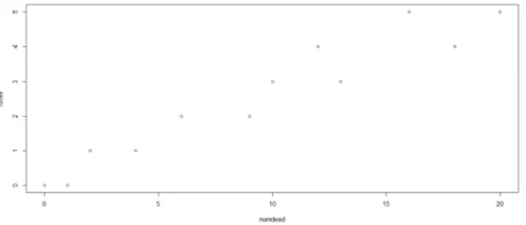
When the “experimental units” are monitored to mortality, modelling the toxicity with GLM assumes that the toxicity increases with the increase in; exposure of the units, dose of the toxic element until when the units get exterminated. The following example illustrates the how the technique works. The data was obtained when groups of 20 male and female moths were exposed to six “increasing” levels of a “pyrethroid” in order to “capture” its toxicity to tobacco budworm. The technique is contained in the following R commands:

> library ("rJava") > library ("glmulti") > ldose<-rep (0:5,2)

> numdead<-c (1,4,9,13,18,20,0,2,6,10,12,16) > sex<-factor (rep(c("M","F"), rep(6,2))) > SF<-cbind (numdead, numalive=20-numdead) > budworm<-glm (SF~sex*ldose, family=binomial) > plot (numdead, ldose)

(3)

Figure 1. Showing the Plot of the Six Increasing Level of dose (i.e. 0 to 5) to the Number of Male (Points Above) and Female (Points Below) Moths that had Died. This Plot was Requested by the Last Command (i.e. “Plot (Numdead, Ldose)”).

The issuance of the commands; > summary(budworm)

> anova(budworm, test="Rao") Will make R to give the result; Call:

glm(formula = SF ~ sex * ldose, family = binomial) Deviance Residuals:

Min 1Q Median 3Q Max -1.39849 -0.32094 -0.07592 0.38220 1.10375 Coefficients:

Estimate Std. Error z value Pr(>|z|) (Intercept) -2.9935 0.5527 -5.416 6.09e-08 *** sexM 0.1750 0.7783 0.225 0.822 Ldose 0.9060 0.1671 5.422 5.89e-08 *** sexM:ldose 0.3529 0.2700 1.307 0.191 ---

Signif. codes: 0 ‘***’ 0.001 ‘**’ 0.01 ‘*’ 0.05 ‘.’ 0.1 ‘ ’ 1 (Dispersion parameter for binomial family taken to be 1) Null deviance: 124.8756 on 11 degrees of freedom Residual deviance: 4.9937 on 8 degrees of freedom

AIC: 43.104

Number of Fisher Scoring iterations: 4 Then the command;

> anova(budworm, test="Rao") Gives the result;

Analysis of Deviance Table Model: binomial, link: logit Response: SF

Terms added sequentially (first to last)

Df Deviance Resid.Df Resid.Dev Rao Pr(>Chi) NULL 11 124.876

sex 1 6.077 10 118.799 6.051 0.0139 * ldose 1 112.042 9 6.757 95.834 <2e-16

*** sex:ldose 1 1.763 8 4.994 1.751 0.1858 ---

Signif. codes: 0 ‘***’ 0.001 ‘**’ 0.01 ‘*’ 0.05 ‘.’ 0.1 ‘ ’ 1 The command;

> summary(glm(SF~sex+ldose,family=binomial)) Will then make R to give the result;

Call:

glm(formula = SF ~ sex + ldose, family = binomial)

Deviance Residuals:

Min 1Q Median 3Q Max -1.10540 -0.65343 -0.02225 0.48471 1.42944 Coefficients:

Estimate Std. Error z value Pr(>|z|) (Intercept) -3.4732 0.4685 -7.413 1.23e-13 *** sexM 1.1007 0.3558 3.093 0.00198 ** Ldose 1.0642 0.1311 8.119 4.70e-16 *** ---

Signif. codes: 0 ‘***’ 0.001 ‘**’ 0.01 ‘*’ 0.05 ‘.’ 0.1 ‘ ’ 1 (Dispersion parameter for binomial family taken to be 1) Null deviance: 124.8756 on 11 degrees of freedom Residual deviance: 6.7571 on 9 degrees of freedom

AIC: 42.867

Number of Fisher Scoring iterations: 4

3.3. When the Organisms are inspected for Information on Toxicity

Here, the organisms (i.e. experimental units) or simply “units” are assembled and samples (e.g. blood and urine samples) are taken from each of them and used to estimate the quantities of the toxic elements available in each of the “sampled” organism. An array of quantities in which columns are allocated to toxic elements and rows, allocated to cases (i.e. units) is the matrix X, in the system of equation (3). The matrix of the response variables Y is usually unknown at the beginning, but with this technique, the matrix X will be used to data-mine some “hidden” information about Y. Such “data-mined” information on Y is either BRV-typed or count data BRV-typed depending on the quantity of hidden information that can be accessed through this technique. If universal “tolerance limits” exist for the units with respect to the toxic elements then a count data type Y is achievable otherwise (i.e. if they exist with respect to some or no toxic element), a BRV type Y is achievable.

3.4. Determination of Matrix Y When Tolerance Limits Exist for all Toxic Elements

(4)

either “ppm” or “µg dL/ ”, in this work; we shall assume the unit is µg dL/ throughout. Each data entry (

x

_ij

,

i

=

1,...,

n

j

=

1,...,

m

) in matrix X is compared with its corresponding tolerance limit (τ_i, i=1, 2,...,m) column-wisely, and instances in which the data entries are greater than their respective tolerance limits are counted and entered as the response variable y_i, i=1,...,n for the corresponding experimental unit. Matrix Y will be “created” the moment we enter the last response variableyn_{. Here, the response matrix Y}

will contain nonnegative integers alone (i.e.

, 0 , 1, 2,...,

i i

y ∈ Ζ ≤y ≤n i= n ). The following section (3.5) contains a vivid numerical illustration of this technique.

3.5. Numerical Illustration on Vulnerability to Toxicity When all Tolerance Limits Exist

Table 1. Showing an Extract of the Matrix X with the Respective Tolerance Limits (Below the Line).

V2 V3 V4 V5 V6 V7 V8 V9

19.64 5.95 0.95 0.74 0.22 0.99 45.37 2.36 18.45 3.77 0.62 0.50 0.12 0.80 23.05 2.19

…

30.1 5.14 1.51 1.24 0.37 0.51 24.89 1.63 28.25 6.30 0.82 0.88 0.20 0.42 17.45 1.16 32.14 5.52 1.06 0.94 0.25 0.57 18.53 1.66

The data for this illustration was obtained through samples from artisans operating in some mechanic villages (along Abeokuta-Ibadan expressways) around Abeokuta metropolis. The toxic elements are eight in number (i.e. V2, V3, …, V9), 118 cases (or units) are used, an extract of the data and their respective tolerance limits are as contained in table 1 below (with all entries measured in µg dL/ );

The corresponding extract of matrix Y (contained in column I or “V1”) is denotedYT =

(

4, 3,..., 4,1

)

. The matrices Y and X are “supplied” together to R, such that the matrix Y occupies the “V1” location and the tolerance limits are excluded. The resulting “data-frame” is named “dat1”. The R codes for this operation are as contained in the three commands below;

If the above three commands are immediately followed by;

>outdat1<-glmulti(V1~V2+V3+V4+V5+V6+V7+V8+V9, data=dat1, method="g", maxit=30)

Then the Genetic algorithmic process to carry-out iterations and identify the formula (model) that will best “fit” the “contents” of dat1 is automatically initialized. An “extract” of the immediate response from R is;

Initialization.

TASK: Genetic algorithm in the candidate set. Initialization.

Algorithm started. After 10 generations: Best model:

V1~1+V5+V7+V8+V3:V2+V4:V2+V5:V4+V6:V2+V6:V5+ V7:V2+V7:V6+V8:V2+V8:V3+V8:V4+V8:V5+V8:V7+V9: V2+V9:V3+V9:V4+V9:V6

Crit= 291.254155883838 Mean crit= 310.663748809868

Change in best IC: -9708.74584411616 / Change in mean IC: -9689.33625119013

After 20 generations: Best model:

V1~1+V7+V3:V2+V5:V2+V5:V4+V7:V2+V7:V3+V7:V6+ V8:V3+V8:V4+V8:V7+V9:V3+V9:V4+V9:V6

Crit= 284.714137298027 Mean crit= 306.254977037995

…

V1~1+V2+V4+V7+V9+V5:V2+V6:V3+V6:V4+V7:V2+V7: V4+V7:V6+V8:V2+V8:V4+V8:V7+V9:V5

Crit= 273.867533645176 Mean crit= 279.11632696666

Improvements in best and average IC have bebingo en below the specified goals.

Algorithm is declared to have converged. Completed.

(5)

Values were Continually Reducing as the Number of Iterations Increases until Convergence was Achieved After 750 Iterations with “Crit= 273.867533645176” and “Mean Crit= 279.11632696666”.

To further show that R’s choice of “Best model” is “reliable” and to carry-on, the researcher needs to give the codes below;

The immediate response of R is as contained in the figure 3 below;

Figure 3. Showing the General Result from the Fitting of the Model (i.e. After Using R’s “Best Model” for Fitting “dat1”).

(6)

had chosen the “simplest” model (as it is usually done without the use of the “glmulti” function), then we would have supplied and receive (output) respectively, the content of figure 4 below;

Figure 4. Showing the Codes with the “Usual” Model (Without Glmulti) and the Corresponding Output.

Notice that;

1. The residual deviance that was 26.106 (with our best model) has now risen to 39.306 (with the usual model) and the AIC that was 411.28 has now risen to 412.48.

2. There is no “over-dispersion”, the evidence for this is contained in figure 5 below;

Figure 5. Showing that There is no Over-dispersion Since the Variance of Y (i.e. 2.542445) is Less than Its Mean (i.e. 3.517) Which is an Unbiased Estimate of the Variance in Poisson Distribution.

(7)

1 3 6 8 1 4 2 5 3 5

1 6 3 6 5 6 1 7 3 7 6 7 4 8

Y = -3.773 + 0.026E + 1.975E + 4.637E + 0.53E + 0.027E E + 0.293E E -4.693E E

-0.102E E -1.68E E + 8.739E E +0.001E E +0.033E E -0.065E E -0.202E E

(4)

WhereE_i, i=1, 2,..., 8, are the data entries per element per artisan and all other coefficients are approximated values of the coefficients in figure 4.

3.6. Further Diagnostic Checks on the Fit for Cases in Which all Tolerance Limits Exist

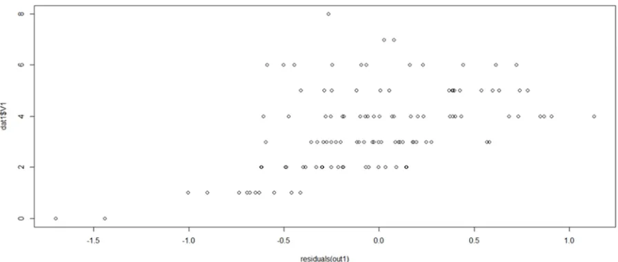
There are other diagnostic checks that corroborate the fact that equation (4) is the best fit for the data (dat1), some of them are; 1. The plot of Y against the residuals which gives the following (figure 3);

Figure 6. Showing That the Plot of Y Against the Residuals does not Connote any Relationship Between Them.

2. By comparing the AIC (for out1), in figure 6, with AIC (for out2), in figure 7, we can easily see that the fit for out1 is better than that for out2. The following pairs of statistics (figure 7) also testify to this fact;

Figure 7. Showing That the Fit for out1 is Better Than That From out2.

3. The “Hosmer and Lemeshow goodness of fit (GOF) test” for out1 (figure 8);

Figure 8. Showing the P-value Equals to 1, Which Means That the Corresponding Fit for out1 Cannot be Due to “Chance” (i.e. the Fit is Reliable) and the X-squared Statistic (i.e -4.3684) is also Good.

The vulnerability to toxicity of each artisan is a probability measure (

P Y

(

=

y

_i

,

i

=

1, 2,...,

n

)

), its numerical value, for the entire data (dat1) will be obtained with the command “log10(fitted(out1)”). An extract of the probabilities is contained

in figure 9 below (i.e. by taken just four decimal places);

Figure 9. Showing an Extract of the Vulnerability to Toxicity of the Artisans.

3.7. Determination of Matrix Y When Tolerance Limits Exist for Some or no Toxic Elements

The determination of the response matrix Y (i.e. a BRV) is through the matrix X which is used to data-mine it, using the following technique; the elements whose tolerance limits exist are “assumed” to be the “main” variables whilst all other variables are “assumed” to be “auxiliary”. In the data matrix X (i.e. in the equation 3), the first toxic element is actually “lead”. Although the human body does not possess any tolerance for lead (i.e. no matter how small the quantity of lead, it is still hazardous to man). However, Nriagu et al. (2008) helped determined the average lead in blood quantity of city children (aged 2 – 9 years) in Ibadan to be

(

9.9±5.2µg dL/

)

_{which depicts that, a non-artisan “child”}

living in Ibadan and its environs could have as much as

(8)

into their body systems. Then a non-artisan adult in Ibadan and its environs is expected to have, on the average, 20

/ g dL

µ of lead in his/her blood. Consequently, if an artisan has above this quantity (i.e. 20µg dL/ ) in his/her blood, we can “safely” assume that the additional quantity is due to occupational toxicity. The value 20 µg dL/ was therefore utilized as the lead (i.e. the main element) toxicity limit for the artisans. By determining toxicity limits for the auxiliary variables (or by using their estimated population mean as toxicity limits), the auxiliary variable were used to “fine-tune” (in the sense that, if four or more of the auxiliary variables are above their toxicity limits, their corresponding yi, i=1,2,…,n that was formally 0 will become 1. Also yi that

was 1 before can become 0 if its main element is within +10 over its toxicity limit and only very few, say one of its auxiliary variable value is more than its toxicity limit) to obtain the concatenated matrix whose extract is;

Figure 10. Showing an Extract of the Concatenated Matrix (Y:X) Which is now the “Input” to R (Below the Line are the Toxicity Limits).

3.8. Numerical Illustration on Vulnerability to Toxicity When Tolerance Limits Exist for Some or no Toxic Elements

The corresponding data-frame is “dat3”, here; Y = yi = 0

or 1 (i.e. 0 denotes that the vulnerability to toxicity is “relatively” low in this particular case when compared with the other cases in the data, whilst yj = 1 denotes it is

relatively high) we now proceed as before to obtain the best model that fits the data as (figure 12);

>

outdat3<-glmulti(V1~V2+V3+V4+V5+V6+V7+V8+V9,data=dat3, method="g", family=binomial)

Initialization.

V1~1+V2+V3+V5+V3:V2+V4:V2+V4:V3+V5:V2+V5:V3+ V5:V4+V6:V4+V6:V5+V7:V3+V7:V4+V7:V6+V8:V5+V8: V6+V8:V7+V9:V3+V9:V7

Crit= 63.9154921762682 Mean crit= 797.229429038279

V1~1+V5+V6+V8+V9+V5:V4+V6:V2+V6:V4+V6:V5+V7: V2+V7:V5+V7:V6+V8:V6+V9:V3+V9:V7+V9:V8

Crit= 47.7447083810335 Mean crit= 58.60998260074

Algorithm is declared to have converged. Completed.

(9)

We now continue with a couple of commands in figure 12. That is;

Figure 12. Showing the Couple of Commands with Which the Model is Fitted and the Result Summarized Before the Display.

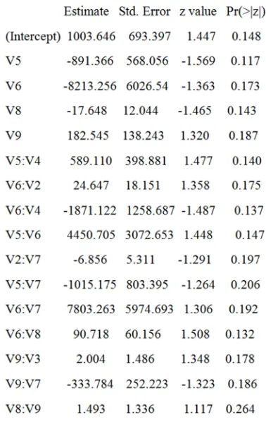
The result is as contained in figure 13 below;

Figure 13. Showing the Result of the Fit for “dat3”.

(10)

4 5 7 8 3 4 1 5

3 5 4 5 1 6 4 6 5 6

5 7 2 8 6

Y = 1003.646 -891.366*E - 8213.256*E -17.648*E +182.545*E +589.11*E * 24.647 * * -1871.122*E *E +4450.705*E *E -6.856*E *E -1015.175*E * 7805.263* *

90.718* * 2.004 * * 333.784 * *

E E E

E E E E E E

+ +

+ + − 8+1.493*E7*E8

(5)

WhereEi, i=1, 2,..., 8, are the data entries per element

per artisan and all other coefficients are approximated values of the coefficients in figure 13.

The vulnerability to toxicity of all the artisans are obtained together through the use of the following three commands (figure 14);

Figure 14. Showing the Three Commands with Which the Vulnerability to Toxicity are Requested for and an Extract of the Corresponding Output.

4. Conclusions

The following conclusions can be reached on the entire work, the issue of the command;

> anova(out1, test="Chisq")

will generate the following “analysis of deviance table” associated with the best fit (frame 11);

Analysis of Deviance Table Model: poisson, link: log Response: V1

Terms added sequentially (first to last)

Figure 15. Showing the Analysis of Deviance Table, It has an Information on the Interaction of Elements; (1 and 4), (3 and 6), (1 and 7) and (6 and 7).

This gives the researcher some hints about some probable interacting toxic elements. Although the response, Y for the

case in which toxicity limits exist for some toxic elements has been coded with 0 and 1, but if it is coded as “FALSE” and “TRUE” (i.e. such that FALSE=0, TRUE=1), it will still work. These results ought to enhance the effectiveness of awareness campaigns informing artisans of the need to always put on their respective “safety” gadgets whenever they are at work. Artisans with high (i.e. TRUE) vulnerabilities to toxicity will know that they really have to exercise caution as much as possible. The results with respect to these coding technique are as contained in the following (figure 16, figure 17);

Figure 16. Showing an Extract of “dat4” that was Supplied to R.

The dat4 was followed by the command;

outdat4<-glmulti(V1~V2+V3+V4+V5+V6+V7+V8+V9,data=dat4,met hod="g", family=binomial)

which initiates the iterations to determine the best model that fits the data (dat4), an extract of the result of which is contained in figure 20 below;

Initialization.

V1~1+V3+V4+V5+V6+V7+V3:V2+V4:V2+V5:V2+V5:V3 +V5:V4+V6:V4+V6:V5+V7:V2+V7:V3+V7:V6+V8:V3+V 8:V5+V8:V6+V8:V7+V9:V4+V9:V8

Crit= 63.9117692465579 Mean crit= 403.601512673779

V1~1+V5+V8+V4:V3+V5:V4+V6:V2+V6:V4+V6:V5+V7: V2+V7:V3+V7:V4+V7:V5+V8:V7+V9:V6

Crit= 43.8845106069435 Mean crit= 63.4907240117881

(11)

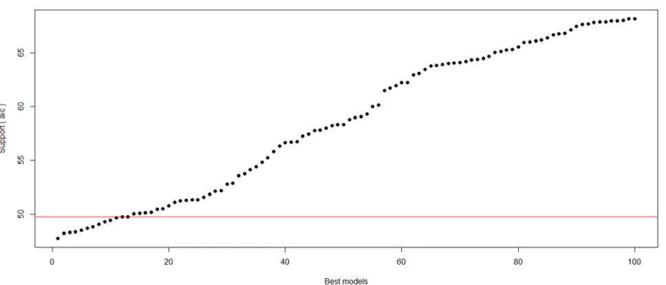
Figure 17. Showing the Extract of the Iteration Process that Identified the Best Model as well as the Corresponding Plot of the Support (aic) Versus Candidate “Best Models”.

With the couple of commands;

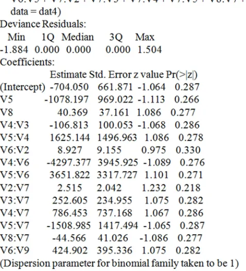
>out4<-glm(V1~1+V5+V8+V4:V3+V5:V4+V6:V2+V6:V4+V6:V5+V7:V2+V7:V3+V7:V4+V7:V5+V8:V7+V9:V6, data=dat4, family=binomial)

> summary(out4)

The following result (i.e. frame 13) was obtained;

Figure 18. Showing the Result of the Fit for dat4.

(12)

4 7 2 3 3 4 1 5

3 5 4 5 1 6 2 6 3 6

4 6 6 7 5 8

704.05 1078.20 * 40.37 * 106.81* * 1625.14 * * 8.93* *

4297.38* * 3651* * 2.52 * * 252.61* * 786.45* *

1508.98* * 44.57 * * 424.90 * *

Y E E E E E E E E

E E E E E E E E E E

E E E E E E

= − − + − + +

− + + + +

− − +

(6)

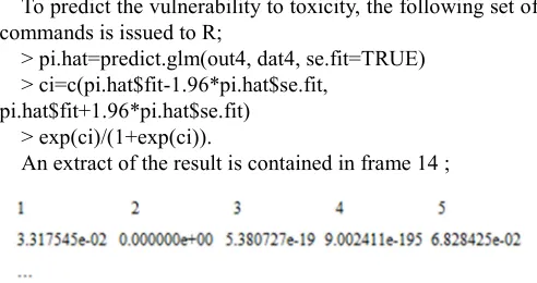
To predict the vulnerability to toxicity, the following set of commands is issued to R;

> pi.hat=predict.glm(out4, dat4, se.fit=TRUE) > ci=c(pi.hat$fit-1.96*pi.hat$se.fit,

pi.hat$fit+1.96*pi.hat$se.fit) > exp(ci)/(1+exp(ci)).

An extract of the result is contained in frame 14 ;

Figure 19. An Extract of the Result on Predicted Vulnerability to Toxicity.

Any of the approaches; depending on the type of data the researcher has (i.e. BRV or count data), could be adopted for any survey work on vulnerability to toxicity.

References

[1] Babalola O O, Okonji R E, Atoyebi J O, Sennuga T F, Raimi M M, Ejim-Eze, E E Adeniran O A, Akinsiku O T, Areola J O, John O O and Odebunmi S O (2010). Distribution of lead in selected organs and tissues of albino rats exposed to acute lead toxicity. Scientific Research and Essay Vol. 5(9), pp.

845-848, Available online at

[2] Calcagno V and Mazancourt C (2010). glmulti: An R Package for easy automated model selection with (generalized) linear models. Journal of statistical software. Volume 34, Issue 12. http://www.jstatsoft.org/

[3] Chege, M W, Rathore, I V S, Chhabra, S C and Mustapha, A O (2009). The influence of meteorological parameters on indoor radon in selected traditional Kenyan dwellings. J. Radiol. Prot. 29 (2009) 95–103.

[4] Dawodu G A, Asiribo O E, Adelakun A A, Ozoje M O,

Ademuyiwa O and Akinwale T A (2011). On the vulnerability of the Blood of some Artisans to Toxicity. Journal of Environmental Statistics. December, 2011, volume 2, Issue 4. http://www.jenstat.org

[5] Dawodu G A (2012). The Derivation of some statistical Models for studying the effects of accidental and occupational pollution. Unpublished PhD (statistics) Thesis submitted to the Department of Statistics, College of Natural Sciences, Federal University of Agriculture, Abeokuta (FUNAAB). [6] Dawodu, G A, Alatise, O O and Mustapha, A O (2015).

Statistical Analysis of Temporal Variations in Indoor Radon Data using an Adapted Response Surface Method. Journal of Natural Science, Engineering and Technology, FUNAAB 14(1):1-12.

[7] Dawodu, G. A. and Mustapha, A. O. (2015). Hierarchical Modelling of Indoor and Outdoor (Residential) Radon Data (RRD). Journal of Natural Sciences, Engineering and Technology, Volume 14 (formally ASSET: An International Journal (Series B)). Published by FUNAAB. Nigeria. (letter of acceptance dated 6th February, 2015).

[8] Kleinbaum D G (1990). Logistic Regression: A self-learning Text. Statistics in the Health sciences. Springer verlag, New York Nriagu J, Afeiche M, Linder A, Arowolo T, Ana G, Mynepalli K C S, Oloruntoba E O, Obi E, Ebenebe J C, Orisakwe O E and Adesina A (2008). Lead poisoning associated with malaria in children of urban areas of Nigeria. International Journal of Hygiene and Environmental Health. doi:10.1016/j.ijheh.2008.05.001.

[9] Ramola, R C, Kandari, M S, Negi, M S and Choubey, V M (2000). A Study of Diurnal Variation of Indoor Radon Concentrations. Journal of Health Physics 35(2); 211-216. [10] Seftelis, L, Nicolaou, G and Trassanidis, S, Tsagas, F N

(2007). Diurnal Variation of Radon Progeny. Journal of Environmental Radioactivity 97, 116-123.