On solving capacitated transportation problem

1. Introduction

The feasible shipment of the products to wholesalers or to warehouses is a common problem in companies. Such problem is called a transportation problem, which is a special case of the linear programming problems. The general model corresponds to the classical transportation problem, comprises of the objective function, supply constraints, demand constraints, and non-negativity constraints. However, if the decision variables which are the amounts of shipment have capacity constraints for various reasons such as capacity of tracks, warehouse capacity, etc., a capacitated transportation model is used.

Capacitated transportation model occurs frequently in applications and it is important to be able to handle the capacity constraints efficiently. This kind of problem can be solved by simplex algorithm for bounded variables [1]. Various authors have studied balanced capacitated transportation problems. Kassay proposed an operator method for solving capacitated transportation problem [7]. Hassain and Zemel studied probabilistic analysis of capacitated transportation problem [6]. They assumed that the capacities are random variables, and provedasymptotic conditions on the supplies and demands which assure that a feasible solution exists almost surely. For studying other researches in this field, one can refer to [2, 8, 13].

 _{Corresponding author}

E-mail address: [email protected] DOI: 10.22105/jarie.2018.133590.1039

On Solving Capacitated Transportation Problem

Kolsoom Ahmadi

Department of Mathematics, Kurdistan University, Sanandaj, Iran.

A B S T R A C T P A P E R I N F O

We present a modification of three existing methods for finding a basic feasible solution for capacitated transportation problem. To obtain an optimal solution, eht simplex algorithm for bounded variables is applied. Special properties of transportation problem help us to operate each step of simplex algorithm directly on the transportation tableau. At last, numerical examples are represented to illustrate our method.

Chronicle:

Received: 26 April 2018 Accepted: 14 July 2018

Keywords: Balanced Transportation Problem.

Capacitated Transportation Problem.

Simplex method, Bounded Variables.

Journal of Applied Research on Industrial

Engineering

Dahiya and Verma considered a class of the capacitated transportation problems with bounds on total availabilities at sources and total destination requirements [3]. They obtained an equivalent balanced capacitated transportation problem for this class of problems. There are several methods for constructing initial basic feasible solutions for transportation problem, i.e. allocating m n 1basic variables which satisfy all constraint equations (e.g. [4, 5, 10, 11]). In capacitated transportation, we have some extra capacity constraints

_,

and the mentioned methods should be modified in order to encase these constraints. We present a modification of three well known methods. In these modified methods, size of the problem does not change, unlike [9] which added a row and a column to the transportation tableau.

In Section 2, we describe the transportation model with bounds on variables and we give a necessary and sufficient condition which assures the feasibility of problem. Section 3 consists of three modified algorithms for constructing an initial basic feasible solution of the problem. Some examples show performance of these algorithms. In Section 4, we explain transportation simplex algorithm for bounded variables to solve one example of the previous section. Comparison the proposed algorithm with an existing algorithm is presented in Section 5. Section 6 contains a short conclusion.

2. Balanced Capacitated Transportation Model

Consider the following balanced transportation

_:

where I {1, 2,, }m is the index set of msources, J {1, 2,, }n is the index set of ndestinations, x_ij

stands for the quantity transported from source i to destination j, c_ij is the cost of transporting one unit between source i and destination j, s_i0 (iI) is the supply of source i, d_j0 (jJ) is the demand of destination j, l_ij0 and we assume _{i j}

i I j J

s d

 



 

. We also have

, , ,

ij j ij i ij j ij i

i I j J i I j J

l d l s u d u s

   

   









to make the problem consistent.

In order to solve problem (1), consider the equivalent transportation problem (2) as follows:

where _{ij ij} , _{i i ij}

i I j J j J

A c l s s l

  







 



and _{j j ij}

i I

d d l



  



.

, ,

ij ij i I j J

ij i j J

ij j i I

ij ij ij

Minimize z c x

subject to x s i I

x d j J

l x u i I j J

            







(1)

0 , , ,

ij ij i I j J

ij i j J

ij j i I

ij ij ij

Minimize z c t A

subject to t s i I

t d j J

t u l i I j J

Clearly, corresponding to every feasible solution t_ij of problem (2), there exists a feasible solution

ij ij ij

x  t l of problem (1), and corresponding to every feasible solution x_ij of (2), there exists a feasible solution t_ijx_ijl_ijof problem (2). The value of the objective function of problem (1) at a feasible solution is equal to the value of theobjective function of (2) at its corresponding feasible solution and conversely. Finally, there is a one-to-one correspondence between optimal solutions to (1) and optimal solutions to (2). Hence, instead of problem (1), we can solve problem (3) as follows

_:

Lemma 1 provides a necessary and sufficient condition for problem (3) to be feasible.

Lemma 1. Problem (3) is feasible if and only if s di j u_ij

d  for all iIand jJ , where

i j

i I j J

d s d

 



 

 .

proof. Suppose that s di j u_ij

d  for all iIand jJ . Set

i j ij

s d x

d

 , we have _{ij i}

j J

x s

 



for all iI,

ij j i I

x d

 



for all jJ and 0x_iju_ij, so x_ij is a feasible solution for (3). Conversely, suppose by

contradiction that ( , )i j I J, . . s t s di j u_ij.

d

    We have _j i j _{ij j},

i I i I

s d

d u d

d

 









 and this is a

violation. So, we should have s di j u_ij

d  for all iIand jJ .

Consider a feasible (3) in which the condition stated in lemma 1 is hold. Since (3) is bounded, there exists at least one optimal solution [1]. We use simplex algorithm for bounded variables to find this optimal solution.

3. Finding an Initial Basic Feasible Solution

To start the transportation simplex, a Basic Feasible Solution (BFS) is needed. There are several methods for obtaining a starting BFS of general transportation in which there aren't upper bounds on variables. In what follows we modify three of the existing methods to make them suitable for capacitated transportation. For a definition of basic feasible solutions of bounded linear programming, see [1].

0 , .

ij ij i I j J

ij i j J

ij j i I

ij ij

Minimize z c x

subject to x s i I

x d j J

x u i I j J

3.1. Modified Northwest Corner Method (MNCM)

This algorithm has two phases:

Phase 1: The algorithm begins withi1 , j1 , sˆ_is_i, dˆ_j d_j.

Step 1:

ˆ ˆ

min{ , , }

ij i j ij

x  s d u .

ˆ ˆ .

ˆi iˆ ij _.

j j ij

s s x d d x

 

 

Step 2:

Case i: xij  sˆi {d uˆj, ij}. i i 1 , j j.

Case ii: xij dˆj{ ,s uˆi ij}. ii, j j 1.

Case iii: x_ij u_ij { ,s dˆ_i ˆ_j}. In this case,x_ij will be non-basic at its upper bound and we will have two new cells. i i 1 , j jand ii , j j 1.

If im j , ngo to Step 3, otherwise go back to Step 1 (In case iii, the algorithm is repeated twice).

Step 3: x_mnmin{ ,s dˆ_m ˆ_n} (Note that sˆ_mdˆ_n since the problem is balanced).

Remark 1: If in one iteration, a row and a column are both satisfied, we move to one of the cells ( ,i j1)or (i1, )j arbitrarily.

Remark 2: If in one iteration of the algorithm, we have one of these three cases: sˆ_idˆ_j 0, ˆs_iu_ij or ˆ

j ij

d u , degeneracy occurs.

When Phase 1 terminates, the last obtaining variable is x_mnsˆ_m dˆ_n. If x_mnu_mn, current solution is feasible otherwise we should go to Phase 2.

Remark 3:The above process can be done similarly if in one step x_ij0. The only difference is that

ij

x

  and the sign of the cells in the cycle starts from positive, since we should increase x_ijto zero. To illustrate the algorithm, we operate it in two numerical examples. The first example goes to Phase 2 and the second one stops at Phase 1.

Example 1: Consider the following capacitated transportation problem:

3 4

1 1

4 4 4

1 2 3

1 1 1

3 3 3 3

1 2 3 4

1 1 1 1

min

15, 25, 40,

10, 23, 22, 25,

ij ij i j

j j j

j j j

i i i i

i i i i

z c x

subject to x x x

x x x x

 

  

   



  

   

















where

11 12 13 14 21 22

23 24 31 32 33 34

4 10 , 5 15 , 1 12 , 3 14 , 1 15 , 5 10,

3 12 , 0 10 , 0 8 , 2 14 , 3 17 , 0 15.

x x x x x x

x x x x x x

           

           

Values of c u_ij, _ijl s d_ij, ,_i _j are shown in Table 1 (c_ij and u_ij l_ij are in the left corner and right corner of the cells, respectively).

Table 1. Values of c uij, ijl s dij, ,i j.

Applying (MNCM) yields the following iterations:

Iteration 1: x₁₁min{2,5,6} 2 , sˆ₁  2 2 0 ,dˆ₁  5 2 3. The next cell is (2,1).

Iteration 2: x₂₁min{16,3,14} 3 , sˆ₂16 3 13 ,   dˆ₁  3 3 0. The next cell is (2,2).

Iteration 3: x₂₂min{13,11,5} 5 , sˆ₂   13 5 8 , dˆ₂  11 5 6. The next cells are (2,3) and (3,2).

Iteration 4.1: x₂₃min{8,15,9} 8 , sˆ₂  8 8 0 , dˆ₃15 8 7. The next cell is (3,3).

Iteration 4.2: x₃₂min{35,6,12} 6 , sˆ₃35 6 29 , dˆ₂  6 6 0. The next cell is (3,3).

Iteration 5: x₃₃min{29,7,14} 7 , sˆ₃29 7 22 , dˆ₃  7 7 0. The last cell is (3,4).

Iteration 6: x₃₄min{22, 22} 22 , sˆ₃dˆ₄0.

1 2 3 4 Supply

1 10 6 12 10 13 11 8 11 2

2 15 14 18 5 12 9 16 10 16

3 17 8 16 12 13 14 14 15 35

The final obtained solution from Phase 1 of (MNCM) is presented in Table 2

;

basic variables are bolded.

Table 2. Obtained solution from Phase 1 of (MNCM).

Since x₃₄22 15 , this solution is not feasible and we should go to Phase 2.

Phase 2:The circle corresponding to the cell (3,4) is {(3,4), (2,4), (2,3), (3,3)} and  7.

Updating variables in the circle yieldsx₃₄7, x₂₄7, x₂₃1, x₃₃14, which is feasible. The obtained BFS is:

Table 3. Obtained solution from Phase 2 of (MNCM).

22 5, 34 15

x  x  . Other nonbasic variables are zero. Since x₃₃14u₃₃, we have degeneracy. The associated transportation cost is:

(2 10) (3 15) (5 18) (1 12) (7 16) (6 16) (14 13) (15 14) 767

z                 .

Example 2: Consider a balanced transportation problem with the same number of variables as the previous example. Values of c u_ij‎‎‎_ijl s_ij‎‎‎ ‎ ‎‎‎ ‎_i d _j are stated in Table 4.

Table 4. Values of c u_ij, _ijl s d_ij, ,_i _j for Example 2.

The final solution which is obtained from Phase 1 of (MNCM) is presented in Table 5

;

basic variables are bolded. Since x₃₄ 9 11, this solution is feasible and the algorithm stops at Phase 1.

2

3 5 8

6 7 22

2

3 1 7

6 14

1 2 3 4 Supply

1 2 10 3 7 4 6 1 9 12

2 -1 5 1 9 3 8 2 7 18

3 5 6 4 7 6 10 3 11 15

Table 5. Obtained solution from Example 2.

The associated transportation cost is:

(5 2) (7 3) (9 1) (8 3) (1 2) (4 4) (2 6) (9 3) 96 z                

3.2. Modified Least Cost Method (MLCM)

This method usually provides a better initial basic feasible solution than the North-WestCorner method, since it takes into account the cost variables in the problem. We should modify the original algorithm in order to deal with bounds of variables. Again the algorithm has two phases.

Phase 1:The algorithmbegins withsˆ_is_i, dˆ_j d_j.

Step 1: Determine cell ( , )i j with the smallest unit cost in the existing tableau. If this cell is not unique, choose one arbitrarily. Set xij min{s d uˆi,ˆj, ij}.

Step 2:

Case i: If x_ij  sˆ_i {d uˆ_j, _ij}, then the i-th row will be crossed out.

Case ii: If x_ij dˆ_j{ ,s uˆ_{i ij}}, then the j-th column will be crossed out.

Case iii: If x_ij u_ij {s dˆ_i,ˆ_j}, then x_ijwill be nonbasic at its upper bound and we should continue searching the smallest unit cost in row iand column j. At last rowior column j will be crossed out.

ˆ ˆ

ˆ_i ˆ_{i ij} , _{j j ij}.

s  s x d d x Go back to Step 1 with the new tableau in which a row or a column is less compare with the previous tableau.

Step 3: When exactly one row or column is left, all the remaining variables are basic. We should have 1

m n  basic variables in total.

Step 4: Suppose that the last remaining cell is ( , )k l . Set x_kl min{ , }s dˆ_k ˆ_l (sˆ_k dˆ_l).

Remark 1: If in one iteration, a row and a column are both satisfied, i.e. sˆidˆj0, then only one of them will be crossed out. It is better to keep the row or column with the smaller c_ijs.

5 7

9 8 1

Remark 2: In case iii, updating sˆ_i and ˆd_jis repeated until one of them becomes zero.

Like the (MNCM), if in one iteration sˆ_i dˆ_j 0, ˆs_iu_ijor ˆd_j u_ij,degeneracy occurs. When Phase 1 terminates, if x_klu_kl, current solution is feasible, otherwise we should go to Phase 2 which is exactly the same as Phase 2 of (MNCM).

Now, we solve Example 1 by (MLCM).

Example 3: Consider the capacitated transportation problem of Example 1. Applying (MLCM), yields: Iteration 1: c₁₄8 is the least unit cost. x₁₄min{2,22,11} 2 , sˆ₁0 , dˆ₄20, cross out row 1.

Iteration 2: c₂₃12 is the least unit cost. x₂₃min{16,15,9} 9 , x₂₃ becomes nonbasic at its upper bound and sˆ₂7 , dˆ₃6. The next cell with the least unit cost in row 2 and column 3 is c₃₃13.

33 min{35,6,14} 6

x   , sˆ₃29, dˆ₃0. Cross out column 3.

Iteration 3: c3414 is the least unit cost. x34min{29,20,15} 15 , x34becomes nonbasic at its upper bound,sˆ₃14 , dˆ₄5. The next cell with the least unit cost in row 3 and column 4 is c₂₄16.

24 min{7,5,10} 5

x   ,sˆ₂2 , dˆ₄ 0.Cross out column 4.

Iteration 4: c2115is the least unit cost. x21min{2,5,14} 2 , sˆ20, dˆ13

.

Cross out row 2.

Iteration 5: Row 3 is the last row, x₃₁and x₃₂will be basic. Since c₃₂c₃₁, we first determine. 32 min{14,11,12} 11

x   , sˆ₃3 , dˆ₂0 and the last variable is x31min{3,3} 3 , sˆ3 dˆ1 0.

Phase 1 terminates and we have x31 3 8, so the current solution is feasible and algorithm stops at Phase 1. The following table shows the result of this example. Basic variables are bolded.

Table 6. Obtained solution of (MLCM).

The associated transportation cost is:

(2 8) (2 15) (9 12) (5 16) (3 17) (11 16) (6 13) (15 14) 749

z                 Which is less than the cost computed by (MNCM).

2

2 9 5

3.3. Modified Vogel's Approximation Method (MVAM)

Vogel's Approximation Method generally yields an optimum or close to optimum solution. The only difference between (MVAM) and (MLCM) is in (MVAM) determining cell ( , )i j with the smallest unit cost is done in a row or column with the largest penalty, not in the entire tableau. This penalty is the difference between two smallest c_ij's in a row or a column.

Example 4: Consider the capacitated transportation problem of Example 1. We explain the first iteration of (MVAM). u_i and v_j stand for penalty of row iand column j, respectively.

Iteration 1: u12, u2 3, u31, v15, v24, v31, v4 6. Column 4 has the largest penalty. The cell with the smallest unit cost in column 4 is (1,4). x₁₄min{2,22,8} 2 , sˆ₁0,dˆ₄20. Cross out row 1.

After completing Phase 1, we have the following BFS. This BFS is just like the BFS which was obtained from (MLCM).

Table 7. Obtained solution of (MVAM).

4. Transportation Simplex for Bounded Variables

The general steps that are taken in simplex method are:

 Finding a starting basic feasible solution.

 Computing z_jc_jfor each nonbasic variables.

 Determining the entering and the leaving variables.

 Updating the basis.

Step 1 was investigated in the previous section. Since for capacitated transportation some of the nonbasic variables may be at their upper bound, entering and leaving basis is a little different; but computing c_ij c_ij z_ij for nonbasic variables is done in a same way [1].

Determining entering variable

Suppose that R₁is the set of indices of nonbasic variables at their lower bound and R₂is the set of indices of nonbasic variables at their upper bound. For determining entering variable, compute

1 2

( , ) ( , )

max{max_{i jR} c_ij , max_{i jR} c_ij}.

  

2

2 9 5

If  0, the current solution is optimal. For  0 suppose that ( , )k l is the index for which the maximum is achieved. If ( , )k l R₁then x_klis increased from its current level of zero. If ( , )k l R₂, then

kl

x is decreased from its current level of ukl.

Determining leaving variable

There exists a unique cycle starting from cell ( , )k l . All corners of this cycle are basic except for ( , )k l . If ( , )k l R₁, we allocate a positive sign to the cell ( , )k l . This sign changes to negative for the adjacent cell and so on. If ( , )k l R₂, sign of the cell ( , )k l is negative and other signs change accordingly. Let

1

T be the set of indices of basic variables in the circle which have positive signs and T₂be the set of indices of basic variables in the circle which have negative signs. Set

1 2

1 min( , )i j T{uij xij} , 2 min( , )i j T{ },xij

       and compute



min{ ,

 

1 2,ukl}.

If

 

 1 the associated basic variable leaves the basis and it will be nonbasic at its upper bound.

If

 

 2 the associated basic variable leaves the basis and it will become zero.

If



ukl the basis doesn't change and xkl is still nonbasic; its bound changes from upper to lower or

vice versa. Only the value of basic variables in the circle will change. Updating the basis

After determining the leaving variable, we should update the variables in the circle by  according to sign of the cells, i.e. x_ij x_ij for ( , )i j with positive sign and x_ij x_ij  for ( , )i j with negative sign.

When we update the transportation tableau, again c_ij's are calculated. This process is done until  0 and we get to optimality.

Example 5: Consider capacitated transportation of Example 1. We apply simplex algorithm starting from the solution of (MVAM). There are two methods for computing c_ij which is not included here (see [1]).

Iteration 1: As you can see in Table 7, we have

       







   



1 1,1 , 1, 2 , 1,3 , 2, 2 , 2 2,3 , 3, 4 .

R  R 

By computing c_ij for nonbasic variables, we have c₁₁3, c₁₂6, c₁₃10, c₂₂4, c₂₃1, c₃₄ 4.

Since sign of the cell

 

2,3 is negative, we have T1{(2,1),(3,3)} and T2{(3,1)}; also 1 min{14 2,14 6} 8



    ,



₂3. Thus  min{8,3,9}3 which is achieved in cell (3,1). x₃₁is the leaving variable and the new values of the variables in the cycle are

23 9 3 6 , 21 2 3 5 , 31 3 3 0 , 33 6 3 9.

x    x    x    x   

The new solution is

Table 8. Optimal solution of Example 1.

Iteration 2: we have R₁



         

1,1 , 1, 2 , 1,3 , 2, 2 , 3,1



, R₂ 



 

3, 4 .



11 3, 12 5, 13 9, 22 3, 31 1, 34 3,

c  c  c  c  c  c   so  max{ 3, 5, 9, 3, 1, 3}        1 0.

The algorithm stops and the current solution is optimal. The optimal transportation cost is: (2 8) (5 15) (6 12) (5 16) (11 16) (9 13) (15 14) 746.

z              

5. Comparison with a Least Cost Method

At first, we state a summary of the classic least cost method for finding an initial feasible solution of capacitated transportation problem [9], then we solve an example by this method and our proposed algorithm.

Finding an initial basic feasible solution

 The cell with the minimum cost in the table is selected and assigned the maximum value possible. If this assignment fully satisfies either the row’s supply or the column’s demand, then the variable is called a basic variable. Otherwise, if the assigned value is limited with the upper bound value of the cell, then it is called a bounded variable. This step is repeated until there exists no possible assignment.

 The table is checked to determine if all of the demands and supplies are fully satisfied. If this is not the case, then a row (row 0) and a column (column 0) are added to the transportation table. Suppose that cell ( , )k l is the last cell in Step 1. A new table is formed with c_k0c_0l1 and c_ij 0 for other cells. The sum of the artificial variables is minimized by simplex method. This step is repeated until artificial variables leave the basis and a feasible solution for the original problem is achieved.

2

5 6 5

Example 6: Consider the following capacitated transportation problem

_.

Table 9. Values of c u_ij, _ijl s d_ij, ,_i _j.

Applied to Table 9, the first step of the mentioned method yields the following assignments; in order

32 20

x  (basic), x₂₃25 (bounded), x₁₃5 (basic), x₃₄5 (basic), x₁₄ 20 (basic), x₂₄10 (basic),

21 7

x  (bounded).

Since the second row and first column still have 8 units unassigned, the solution is not feasible. Iteration 1: The sum of artificial variables x₂₀x₀₁ should be minimized over the following table.

Table 10. Transportation table of Iteration 1.

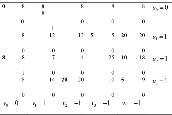
Basic variables are bolded, u_ij l_ij s are in the right corner of the cells. All c_ij s are zero except for c₀₁ and c₂₀ which are equal to 1. u_i and v_j are calculated in the right and below of the table. Computing

ij

c by MODI method yields c02c03c041 , c10 1 , c11 2 , c120 , c21 2, 22 23 0 , 30 1 , 31 2 , 32 0.

c c  c   c   c 

2

  , x₃₁ is the entering variable and the corresponding cycle is

           



3,1 , 3, 4 , 2, 4 , 2,0 , 0,0 , 0,1 . We have



 min{5,8}5 and x34 should leave the basis. After

updating the variables in the cycle, we have the following table.

1 2 3 4 Supply

1 10 12 5 13 6 5 7 25 25

2 9 7 3 4 4 25 8 18 50

3 8 14 2 20 7 10 6 9 25 Demands 15 20 30 35

0 8

0 8 8 1 8 0 8 0 8 0 0 0 u  8 0 12 0 13 0

5 5

0

20 20

0

1 1

u 

8 8

1 7 0 4 0 25 0

10 18

0 2 1 u  8 0 14 0

20 20

0

10

0

5 9

0

3 1 u 

0 0

Table 11. Transportation table of Iteration 2.

Iteration 2:

02 1 , 03 04 1 , 10 1 , 11 12 21 22 2 , 23 0 , 30 1 , 33 34 2

c   c c  c   c c c c   c  c  c c 

 2. x₁₁ is the entering variable and the corresponding cycle is

           



1,1 , 1, 4 , 2, 4 , 2,0 , 0,0 , 0,1 . We have



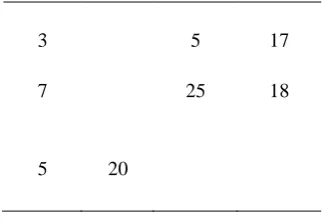
 min{3,8, 20}3. After updating variables in the cycle, the new value of artificial variables x₀₁ and x₂₀ will be zero and we get to a feasible solution of the original problem which can be seen in Table 12. x₂₁7 and x₂₃25 are bounded variables.

Table 12. Feasible solution of Least Cost Method.

The associated transportation cost is:

(3 10) (5 6) (17 7) (7 9) (25 4) (18 8) (5 8) (20 2) 566. z                

Finding initial basic feasible solution by (MLCM)

Phase 1 of (MLCM) method generates the following solution:

5 8

0

3 8

1

8 0 8 0 8 0 0 0 u  8 0 12 0 13 0 5 5

0 20 20

0 1 1 u  3 8

1 7 0 4 0 25 0 15 18

0 2 1 u  8 0 5 14

0 20 20

0 10 0 9

0

3 1

u  

0 0

v  v₁1 v₂ 1 v₃ 1 v₄ 1

3 5 17

7 25 18

Table 13. Obtained solution of phase 1 of (MLCM) for example 6.

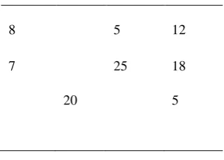
Sincex₂₁15 7 , Phase 2 is performed.The circle corresponding to the cell (2,1) is {(2,1), (2,4), (1,4), (1,1)} and  8. Updating variables in the circle yieldsx₂₁7, x₂₄ 18, x₁₄12, x₁₁8 which is feasible. The obtained BFS is:

Table 14. Obtained solution from Phase 2 of (MLCM).

The associated transportation cost is:

(8 10) (5 6) (12 7) (7 9) (25 4) (18 8) (20 2) (5 6) 571. z                

As it is evident from the above example, our proposed algorithm generates a feasible solution for capacitated transportation problem with less computations and without changing size of the problem. The mentioned Least Cost Method needs some simplex iterations to get to a starting feasible solution; but our proposed method obtains a feasible solution just by one or some updating steps in Phase 2.

6. Conclusion

Capacitated transportation problem is a special case of bounded linear programming problems. It has many practical applications in various areas including inventory control, employment scheduling, telecommunication networks, and personnel assignment. In this research, we used three methods

_:

Modified Northwest Corner Method (MNCM), Modified Least Cost Method (MLCM), and Modified Vogel's Approximation Method (MVAM) to find an initial BFS of this problem. For obtaining optimal solution of the problem, the simplex algorithm with detailed explanation used. All steps of our method operate directly on the table and we don't need to add any row or column to the tableau.

References

[1] Bazaraa, M. S., Jarvis, J. J., & Sherali, H. D. (2011). Linear programming and network flows. John Wiley & Sons.

[2] Bit, A. K., Biswal, M. P., & Alam, S. S. (1993). Fuzzy programming technique for multi objective capacitated transportation problem. Journal of fuzzy mathematics, 1(2), 367-376.

5 20

15 25 10

20 5

8 5 12

7 25 18

[3] Dahiya, K., & Verma, V. (2007). Capacitated transportation problem with bounds on rim conditions. European journal of operational research, 178(3), 718-737.

[4] Goyal, S. K. (1984). Improving VAM for unbalanced transportation problems. Journal of the operational research society, 35(12), 1113-1114.

[5] Hakim, M. A. (2012). An alternative method to find initial basic feasible solution of a transportation problem. Annals of pure and applied mathematics, 1(2), 203-209.

[6] Hassin, R., & Zemel, E. (1988). Probabilistic analysis of the capacitated transportation problem. Mathematics of operations research, 13(1), 80-89.

[7] Kassay, F. (1981). Operator method for transportation problem with bounded variables. Prace a\v studie vysokej\v skoly dopravy spojov v\v ziline séria matematicko-fyzikalna, 4, 89-98.

[8] Rachev, S. T., & Olkin, I. (1999). Mass transportation problems with capacity constraints. Journal of applied probability, 36(2), 433-445.

[9] Rachev, S. T., & Olkin, I. (1999). Mass transportation problems with capacity constraints. Journal of applied probability, 36(2), 433-445

[10] Spivey, W., & Thrall, R. (1970). Linear Optimization. Inc., New York, NY: Holt, Rinehart and Winston. [11] Sudhakar, V. J., Arunsankar, N., & Karpagam, T. (2012). A new approach for finding an optimal solution

for transportation problems. European journal of scientific research, 68(2), 254-257. [12] Taha, H. A. (2003). Operations research: An introduction Seventh edition. Prentice Hall