R E S E A R C H
Open Access
Accounting for biases in survey-based
estimates of population attributable
fractions
Ryan Masters
1*and Eric Reither
2Abstract
Background:This paper discusses best practices for estimating fractions of mortality attributable to health exposures in survey data that are biased by observed confounders and unobserved endogenous selection. Extant research has shown that estimates of population attributable fractions (PAF) from the formula using the proportion of deceased that is exposed (PAFpd) can attend to confounders, whereas the formula using the proportion of the
entire sample exposed (PAFpe) is biased by confounders. Research has not explored how PAFpdand PAFpe
equations perform when both confounding and selection bias are present.
Methods:We review equations for calculating PAF based on either the proportion of deceased (pd) or the
proportion of the entire sample (pe) that receives the exposure. We explore how estimates from each equation are affected by confounding bias and selection bias using hypothetical data and real-world survey data from the National Health Interview Survey–Linked Mortality Files, 1987–2011. We examine the association between cigarette smoking and all-cause mortality risk in the US adult population as an example.
Results:We show that both PAFpdand PAFpecalculate the true PAF in the presence of confounding bias if one
uses the“weighted-sum”approach. We further show that both the PAFpdand PAFpecalculate biased PAFs in the
presence of collider bias, but that the bias is more severe in the PAFpdformula.
Conclusion:We recommend that researchers use the PAFpeformula with the weighted-sum approach when
estimates of the exposure-outcome relationship are biased by endogenous selection.
Keywords:Attributable fractions, Selection bias, Confounding bias, Mortality
Background
This paper discusses best practices for estimating the fraction of mortality attributable to health exposures in survey-based data that are biased by both observed con-founders and unobserved endogenous selection. Much extant work has reviewed errors in computing popula-tion attributable fracpopula-tions (PAFs) in the presence of con-founders [1–6], but little work has considered how different formulae for computing PAFs are affected by endogenous selection biases (e.g., collider bias).
Endogenous selection bias can affect estimates of statistical associations in many ways. Conditioning on a
collider variable—that is, a variable caused by two other variables that are associated with the exposure and the outcome—can occur through statistical control, stratifi-cation of the sample into different groups, or the selec-tion of participants into a study [7–11]. Introducing collider variables through any of these mechanisms can bias estimates of associations between exposure and out-come. In this study, we focus onunobservedendogenous selection—a problem that commonly occurs in health studies through the sampling process of recruiting study participants. Simply put, the likelihood of participation in a health study can be affected by both the exposure and outcome, which can bias estimates of the true asso-ciation between them.
The most common PAF formulae are based on either the proportion of deceased (pd) in the sample that
© The Author(s). 2019Open AccessThis article is distributed under the terms of the Creative Commons Attribution 4.0 International License (http://creativecommons.org/licenses/by/4.0/), which permits unrestricted use, distribution, and reproduction in any medium, provided you give appropriate credit to the original author(s) and the source, provide a link to the Creative Commons license, and indicate if changes were made. The Creative Commons Public Domain Dedication waiver (http://creativecommons.org/publicdomain/zero/1.0/) applies to the data made available in this article, unless otherwise stated.
* Correspondence:ryan.masters@colorado.edu
1Department of Sociology, Population Program and Health & Society
Program, Institute of Behavioral Sciences, University of Colorado Population Center, Boulder, CO 80309, USA
receives the exposure or the proportion of the entire sample (pe) that receives the exposure [1]. The two main aims of this investigation are to examine the perform-ance of these model-based methods for calculating PAF in the presence of (1) known and observable con-founders of the exposure-mortality association and (2) collider bias. We focus on the association between cigarette smoking and all-cause mortality risk in the US adult population, which is confounded by other variables and also a likely contributor to unobserved endogenous selection bias in survey-based data of smoking and mor-tality risk [7].
Methods
We use hypothetical data and real-world survey data to calculate PAF in the presence of confounding and unob-served endogenous selection. In all of our exercises, non-exposed cases are respondents who have never smoked cigarettes and exposed cases are respondents who are current or former smokers. The association of interest is how smoking affects all-cause mortality risk. For each exercise, we estimate the fraction of US mortal-ity attributable to cigarette smoking using the PAFpd
formula:
PAFpd¼ðpdðRR−1ÞÞ=RR ð1Þ
where pd is the prevalence of a health exposure among the deceased cases and RR is the mortality risk ratio be-tween the exposed and non-exposed subjects [12]. We also estimate this fraction using the PAFpeformula:
PAFpe¼ðpeðRR−1ÞÞ=ð1þðpeðRR−1ÞÞÞ ð2Þ
where pe is the prevalence of the exposure among all cases in the sample [6,13]. For each formula, we adopt a “weighted-sum” approach [1, 3, 14, 15], which uses model-based adjusted estimators of PAF separately for each adjustment level i as well as the distribution of cases by the adjustment levels:
PAFpd¼
X
WiðpdiðRRi−1ÞÞ=RRi ð3Þ
PAFpe¼
X
WiðpeiðRRi−1ÞÞ=ð1þpeiðRRi−1ÞÞ
ð4Þ
where i indicates the adjustment level (i.e., con-founder) and Wi indicates the proportion of deaths in
adjustment leveli. The weighted-sum approach is math-ematically equivalent to the PAFpd [1, 14]; combining
the PAFpd with the weighted-sum approach is therefore
redundant. Nevertheless, we apply it in all of our exer-cises to maintain consistency.
Exercise 1: Observed confounding bias in hypothetical data
In our first exercise, we examine PAF estimates from Eqs. (1–4) in the presence of a single confounder, race/ ethnicity. For simplicity, we consider race/ethnicity using only two categories, Hispanic black and non-Hispanic white (hereafter black and white). The hypo-thetical data are composed of 1000 black respondents and 4000 white respondents. Both smoking prevalence (i.e., pe) and mortality risk are higher among black re-spondents than among white rere-spondents, which con-found the smoking-mortality association. In these data, black pe is 0.35 compared to white pe of 0.2, and overall mortality risk for black respondents is 0.3 compared to 0.2 for white respondents.
Exercise 2: Unobserved endogenous selection bias in hypothetical data
Our second example uses the same data as before, but presupposes that estimates of the smoking-mortality association are biased by differential selection into the sample. We assume that current smokers sampled are relatively more select on health than are non-smokers. That is, both the non-smoking and the smoking samples are healthier than the true populations, but the differ-ence between the smoking sample and the smoking population is greater than the difference between the non-smoking sample and the non-smoking population. This unobserved process of health selection biases downward the all-cause mortality RR estimated in the sample data. When these conditions hold, both PAF esti-mates will be biased due to the central role of the RRs (see Eqs. 1–4). Moreover, the distribution of deaths by exposure and by adjustment levels, Wi, will also be
biased. This is because counts of deaths among the ex-posure group in the sample will be artificially low and, consequently, Wi will be incorrect. Thus, PAFpd and
PAFpe estimates will remain biased via Wi even if our
adjusted RRs account for collider bias. Finally, the esti-mated PAF from the PAFpdformula will be additionally
biased, due to the central role of the pd in the calcula-tion of the PAF. That is, the pd in the observed data, like the RRs in the observed sample data, will be downwardly biased because deaths among the smoking sample are underreported.
waves from 1987 and 1989–2009 that have been linked to official death records at the National Death Index through December 31, 2011 (the 1988 NHIS survey did not contain information about respondents’smoking be-havior). The NHIS-LMF are designed to form a repre-sentative sample of non-institutionalized US adults [12]. To simplify the example, we limit the analytic sample to contain only US adult black and white men and women aged 40 through 84 at time of interview and whose sur-vival is followed between ages 50 and 84. We extend the example by considering two levels of smoking exposure, “former smoker”and“current smoker,”and by consider-ing three possible confounders of the smokconsider-ing-mortality association: race/ethnicity (i.e., white and black), gender (i.e., men and women), and age group (i.e., 50–59, 60– 69, 70–79, and 80–84).
We fit a series of clog-log discrete-time survival models to estimate smoking-based differences in US adult mortality risk. First, we fit a baseline model that estimates differences in mortality risks between current, former, and never smokers (reference category). Next, we fit aconfoundermodel that estimates age-specific dif-ferences in mortality risks between current, former, and never smokers, adjusting for race/ethnicity and gender as categorical confounders of the smoking-mortality as-sociation. We also fit models separately for black and white men and women that estimate age-specific RRs for former and current smokers compared to never smokers (i.e., confounder-specific models to be used with the weighted-sum approach to calculate PAFs). Finally, we fit a biasmodel that refits the confounder model by ac-counting for cohort-based variation in mortality risk and age-related selection biases in the NHIS-LMF data.
Participants in health surveys like the NHIS are positively selected on survival, health, and non-institutional living ar-rangements [16]. These selection biases tend to grow stron-ger with increasing age [17]. Thus, older respondents in NHIS-LMF data are selected on the outcome of interest (i.e., survival) and inclusion in the NHIS sampling frame (i.e., healthy and living in non-institutionalized housing). Combined, the selective nature of the sample results in col-lider biases via age-related selection into the sampling frame and the selective factors associated with age are likely stronger among respondents with health risk factors such as smoking than among healthy respondents [8].
Survival models fitted separately by cohort of entry into the NHIS sample provide evidence consistent with these assumptions about collider biases. For example, the esti-mated RR between current smokers and never smokers who died at age 70–80 ranges from 1.51 [1.43–1.58 95%CI] among respondents surveyed at age 70–75 to 4.11 [3.02–5.57 95%CI] among respondents surveyed at age 50–55. The bias model is a shared frailty survival model that estimates random effects variation in mortality risk by
NHIS respondents’5-year age cohorts at the time of sam-pling. Overall, the model fits age-specific mortality risks separately for current, former, and never smokers, adjust-ing for gender, race/ethnicity, birth year, and random ef-fects for a 5-year cohort of entry into the data.
Mortality differences between US adults self-reported to be current, former, and never smokers between ages 50 and 84 are estimated across these three models. We use the adjusted RRs between (1) current smokers and never smokers and (2) former smokers and never smokers, which are estimated from confounder-specific survival models and the weighted-sum approach to calculate the PAF for smoking as a cause of death in the US adult black and white populations between ages 50 and 84 for years 1987–2011. For all models, we contrast PAFs calculated from PAFpdwith PAFs calculated from PAFpeto examine
how each formula is affected by (1) confounders in the es-timated smoking-mortality association and (2) collider bias.
The NHIS-LMF data analyzed for the current study are public-use files made available by the NCHS (https:// www.cdc.gov/nchs/data-linkage/mortality.htm). The ana-lytic scripts (Additional file1) and calculations to gener-ate results (Additional file 2) for Exercise 3 are available in the appendix.
Results
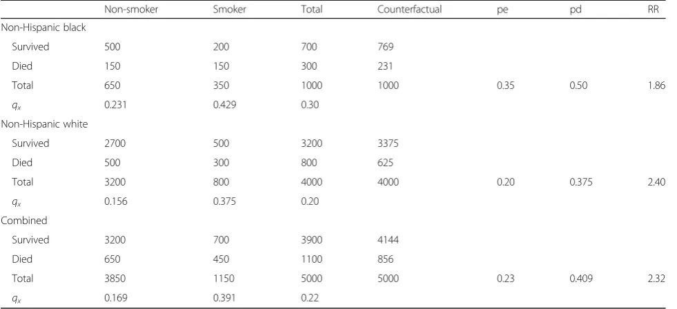
Exercise 1: Observed confounding in hypothetical data The confounding effect of race/ethnicity on the smoking-mortality association is illustrated in Table 1. The all-cause mortality RR for smoking when unadjusted for the confounding effects of race/ethnicity is (450/1150)/(650/ 3850) = 2.32. Alternatively, the RR adjusted for race/ethni-city is 2.23. That is, when we estimate separate RRs for each race/ethnicity sample, we observe
Non−Hispanic black¼ð150=350Þ=ð150=650Þ ¼1:86
Non−Hispanic white¼ð300=800Þ=ð500=3200Þ ¼2:40
When these race/ethnic-specific RRs for smoking are standardized by the race/ethnic distribution of deaths and the race/ethnic distribution of smoking prevalence, the adjusted RR is 2.23. If one does not account for the confounding effects of race/ethnicity on both mortality risk and the probability of smoking, one would incor-rectly estimate the PAF by the following:
a) Aggregating the probability of smoking to be (1150/ 5000) = 0.23,
c) Aggregating the RR associated with smoking to be (450/1150)/(650/3850) = 2.32.
As a result, estimates of the PAF for smoking, irre-spective of the formula used, would be biased by not at-tending to the confounding effects of race/ethnicity:
PAFpd¼ðpdðRR−1ÞÞ=RR¼ð0:41ð2:32−1ÞÞ=2:32
¼0:233
PAFpe¼ðpeðRR−1ÞÞ=ð1þðpeðRR−1ÞÞÞ
¼ð0:23ð2:32−1ÞÞ=ð1þð0:23ð2:32−1ÞÞÞ ¼0:233
The actual PAF shown in the counterfactual example above is (1100−856)/1100 = 0.222
Thus, by failing to account for (1) the higher preva-lence of smoking among black respondents and (2) the higher mortality risks among black respondents, we would incorrectly inflate the RR associated with smoking and misattribute numerous deaths to smoking as a cause of mortality in the population. As such, it is necessary to identify the RR by accounting for confounders in model estimates, and then use this confounder-adjusted RR to calculate PAFs [18]. It has been argued that only the PAFpd formula can accurately estimate the PAF when
using confounder-adjusted RRs [3–6]. Yet, as others have noted, one can use the PAFpe equation with the
confounder-adjusted RR to derive the true PAF [1, 15]. To do so, one needs to first estimate separate PAFs for each confounder group (i.e., each adjustment level i),
and then standardize these confounder-specific PAFs by the distribution of deaths across groups (i.e.,Wi).
To illustrate, when we estimate separate PAFs for black and white respondents, we see for black:
PAFpd¼ðpdðRR−1ÞÞ=RR¼ð0:5ð1:86−1ÞÞ=1:86
¼0:231
PAFpe¼ðpeðRR−1ÞÞ=ð1þðpeðRR−1ÞÞÞ
¼ð0:35ð1:86−1ÞÞ=ð1þð0:35ð1:86−1ÞÞÞ ¼0:231
and for white:
PAFpd¼ðpdðRR−1ÞÞ=RR¼ð0:375ð2:40−1ÞÞ=2:40
¼0:219
PAFpe¼ðpeðRR−1ÞÞ=ð1þðpeðRR−1ÞÞÞ
¼ð0:2ð2:40−1ÞÞ=ð1þð0:2ð2:40−1ÞÞÞ ¼0:219
To estimate the total PAF, we further attend to the distribution of deaths across groups. That is, we sim-ply weight the confounder-specific PAFs by the pro-portion of total deaths occurring in the confounder groups (i.e., Wi) [18]. The proportion of the total
deaths that occurred among black respondents = (300/ 1100) = 0.273 and the proportion of total deaths that occurred among white respondents = (800/1100) = 0.727. When we weight the confounder-specific PAFs by the proportion of deaths in the two groups,Wi, we
retrieve the true overall PAF:
Table 1Hypothetical sample data
Non-smoker Smoker Total Counterfactual pe pd RR
Non-Hispanic black
Survived 500 200 700 769
Died 150 150 300 231
Total 650 350 1000 1000 0.35 0.50 1.86
qx 0.231 0.429 0.30
Non-Hispanic white
Survived 2700 500 3200 3375
Died 500 300 800 625
Total 3200 800 4000 4000 0.20 0.375 2.40
qx 0.156 0.375 0.20
Combined
Survived 3200 700 3900 4144
Died 650 450 1100 856
Total 3850 1150 5000 5000 0.23 0.409 2.32
qx 0.169 0.391 0.22
PAFNHBWNHBþPAFNHWWNHW
¼ð0:2310:273Þ þð0:2190:727Þ ¼0:222
This shows that the weighted-sum approach can cal-culate the true PAF regardless if one uses the PAFpd or
PAFpeformula. So long as (1) unobservable confounders
or unobservable selection do not induce bias, and (2) one attends to observable confounders of the smoking-mortality association, one can use adjusted RRs with ei-ther PAFpdor PAFpeand the weighted-sum approach to
calculate the PAF for smoking-related mortality in the sample [18].
Exercise 2: Unobserved endogenous selection in hypothetical data
In the next exercise, we extend the previous example to consider sample data that are biased by unobserved se-lection, causing underestimation of mortality risk in the smoking population. To simplify matters, let us assume that the prevalence of smoking is the same in both the sample and population so that the only change pertains to qx for smokers in the sample. The new information
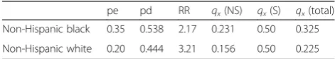
about population parameters is presented in Table 2 below.
The mortality probabilities for the non-smoking popu-lations equal those in the sample data (0.231 among blacks and 0.156 among whites). Smoking prevalence is also the same (peNHB = 0.35 and peNHW = 0.20).
How-ever, we now see discrepancies in the mortality risks for the smoking populations (0.500 in the white population vs. 0.375 in the white sample, and 0.500 in the black population vs. 0.429 in the black sample). These, in turn, affect the RRs for smoking (e.g., 2.17 vs. 1.86 for black and 3.21 vs. 2.40 for white), the pds (0.538 vs. 0.500 for black and 0.444 vs. 0.375 for white), and the Wi (e.g.,
0.265 of population deaths are among blacks vs. 0.273 of sample deaths).
The confounder-specific PAFs using both the PAFpd
and PAFpe formulae are as follows (estimates might be
slightly different due to rounding): non-Hispanic black:
PAFpd¼ðpdðRR−1ÞÞ=RR¼ð0:538ð2:17−1ÞÞ=2:17
¼0:290
PAFpe¼ðpeðRR−1ÞÞ=ð1þðpeðRR−1ÞÞÞ
¼ð0:35ð2:17−1ÞÞ=ð1þð0:35ð2:17−1ÞÞÞ ¼:290
non-Hispanic white:
PAFpd¼ðpdðRR−1ÞÞ=RR¼ð0:444ð3:21−1ÞÞ=3:21
¼0:306
PAFpe¼ðpeðRR−1ÞÞ=ð1þðpeðRR−1ÞÞÞ
¼ð0:20ð3:21−1ÞÞ=ð1þð0:20ð3:21−1ÞÞÞ ¼0:306
Standardizing these confounder-specific PAFs by the distribution of deaths, Wi, we use the weighted-sum
ap-proach to calculate the true PAF:
0:2900:2653
ð Þ þð0:3060:7347Þ ¼0:301
We see that the PAFs in the sample data underesti-mate the true PAF in the population (0.222 vs. 0.301), and this bias is the same in the PAFpdand PAFpe
formu-lae. The discrepancy arises from one’s inattention to (unobservable) endogenous selection bias in the sample data, resulting in biased sample estimates of the mortal-ity RRs associated with smoking as well as biasedWi in
the sample.
Imagine that we had accounted for unobservable selec-tion bias in our survival models and correctly identified the RRs for smoking for both the black and white sam-ples. Even though the adjusted RRs would be correct in our survival models, the counts of deaths in the sample data would remain biased. Consequently, the pd values in the sample stay at 0.50 and 0.375, and the proportion of deaths occurring among blacks and whites stay at 0.273 and 0.727, respectively. As a result, if we were to calculate the PAF using the adjusted RRs with PAFpd, we
would find
PAFpdb¼ðpdðRR−1ÞÞ=RR¼ð0:50ð2:17−1ÞÞ=2:17
¼0:270
PAFpdw¼ðpdðRR−1ÞÞ=RR
¼ð0:375ð3:21−1ÞÞ=3:21¼0:258
The confounder-specific PAFs are biased (i.e., 0.270 estimated vs. 0.290 actual for blacks and 0.258 estimated vs. 0.306 actual for whites) even when using the adjusted RRs. Furthermore, when we use the weighted-sum ap-proach and standardize these PAFs by Wi, we add
an-other source of bias because the distribution of deaths in each confounder group is biased as well: total PAF = (0.270*0.273) + (0.258*0.727) = 0.263. Yet, were we to follow conventional wisdom [3–6] and use the adjusted
Table 2Hypothetical population data
pe pd RR qx(NS) qx(S) qx(total)
Non-Hispanic black 0.35 0.538 2.17 0.231 0.50 0.325
Non-Hispanic white 0.20 0.444 3.21 0.156 0.50 0.225
peproportion smoker in population,pdproportion smoker among deceased
in population,qx(NS)probability of death among nonsmokers in population,
RR with the PAFpdfor the entire sample, we would
esti-mate the same biased PAF:
PAFpd¼ðpdðRR−1ÞÞ=RR
¼ðð450=1100Þð2:8−1ÞÞ=2:8¼0:263
Thus, even if we accurately accounted for selection bias in our survival models and estimated an unbiased RR (e.g., by fitting frailty models that account for selec-tion bias in the smoking RR [19]), the PAF calculated from the PAFpdformula will still be biased. In this case,
a biased 0.263 is estimated for the sample when the true PAF in the population is 0.301 (a bias on the proportion-ate scale of 12.6%: (0.263−0.301)/0.301).
If we calculate the PAF using the confounder- and selection-adjusted RRs with the PAFpeformula, we find
PAFpeb¼ðpeðRR−1ÞÞ=ð1þðpeðRR−1ÞÞÞ
¼ð0:35ð2:17−1ÞÞ=ð1þð0:35ð2:17−1ÞÞÞ ¼0:290
PAFpew¼ðpeðRR−1ÞÞ=ð1þðpeðRR−1ÞÞÞ
¼ð0:2ð3:21−1ÞÞ=ð1þð0:2ð3:21−1ÞÞÞ ¼0:306
We see that the confounder-specific PAFs are un-biased. Only when we standardize these PAFs by the dis-tribution of deaths, Wi, do we introduce slight bias in
the total PAF = (0.290*0.273) + (0.306*0.727) = 0.302 (a bias on the proportionate scale of − 0.3%: (0.301 − 0.302)/0.302). Thus, when we account for selection bias in our survival models and estimate unbiased adjusted RRs, the PAF calculated from PAFpe will be biased, but
only viaWi. By using the PAFpeequation, we avoid bias
in estimates from the pd and dramatically reduce the overall bias in the PAF estimate (0.3% vs. 12.6%).
To recap, when sample data are biased by unobserved selection, both the PAFpdformula and the PAFpeformula
will calculate a biased PAF—even if researchers adjust for selection bias in the data. However, the PAFpdformula is
far more affected by the bias than is the PAFpeformula
be-cause bias is introduced in both the pd and Wi.
Con-versely, estimates of the confounder-specific PAF from the PAFpe equation are not biased, but some bias is
intro-duced in the weighted-sum approach via Wi.
Theoretic-ally, one could completely eliminate bias by identifying the true RR (i.e., attend to both observable confounders and unobservable selection biases) and standardizing the PAFs by the true distribution of deaths for each adjustment level (i.e., use population data to estimateWi).
Exercise 3: PAF estimation with real-world survey data For the final exercise, we calculate PAF for smoking as a cause of US adult mortality in the NHIS-LMF data, which are biased by confounding (i.e., age, race/ethnicity, and gender) and likely biased by endogenous selection (i.e., likelihood of sample inclusion depends on health). Table 3shows age-specific mortality risks between years 1987 and 2011 for NHIS respondents who are current, former, and never smokers. The pd for former smokers (0.352) combined with the pd for current smokers (0.338) indicates that nearly 70% of the deceased NHIS sample had been exposed to smoking.
From the sample data in Table3, we calculate the un-adjusted RRs:
Total RRformer¼ð14;566=92;693Þ=ð12;816=121;459Þ
¼1:489
Total RRcurrent¼ð13;984=86;969Þ=ð12;816=121;459Þ
¼1:524
Because we are calculating a PAF for two-levels of an exposure, former smokers and current smokers, the PAF formulae change slightly [18,20]:
PAFpd¼pdformerðRRformer−1Þ=RRformer
þpdcurrentðRRcurrent−1Þ=RRcurrent
Table 3Age-specific mortality counts by smoking exposure level, NHIS-LMF 1987–2009
Age Dead Total qx pe pd
Never smokers
50 1169 43,737 0.027 0.403 0.243
60 2109 41,443 0.051 0.396 0.233
70 4833 26,249 0.184 0.401 0.299
80 4705 10,030 0.469 0.451 0.414
Total 12,816 121,459 0.106 0.403 0.310
Former smokers
50 959 27,283 0.035 0.251 0.200
60 2624 32,554 0.081 0.311 0.289
70 6310 24,207 0.261 0.369 0.391
80 4673 8649 0.540 0.389 0.412
Total 14,566 92,693 0.157 0.308 0.352
Current smokers
50 2674 37,632 0.071 0.346 0.557
60 4335 30,727 0.141 0.293 0.478
70 4998 15,067 0.332 0.230 0.310
80 1977 3543 0.558 0.159 0.174
PAFpe¼ ðpeformerðRRformer−1Þ
þpecurrentðRRcurrent−1ÞÞ=ð1þ ðpeformerðRRformer−1Þ
þpecurrentðRRcurrent−1ÞÞÞ
PAFpd¼0:352ð1:489−1Þ=1:48
þ0:338ð1:524−1Þ=1:52 ¼0:232
PAFpe¼ ð0:308ð1:489−1Þ
þ0:289ð1:524−1ÞÞ=ð1þ ð0:308ð1:489−1Þ þ0:289ð1:524−1ÞÞÞ ¼0:232
We see that if we did not consider age, race/ethnicity, or gender as confounders of the smoking-mortality asso-ciation in these NHIS-LMF data, we would estimate about 23% of US black and white adult deaths between ages 50 and 85 for years 1987–2011 were attributable to cigarette smoking.
Average RRs for current smoking estimated from clog-log discrete time hazard models are presented in Table4, and overall PAFs estimated from the PAFpe and PAFpd
formula are included as well.
The baseline model estimates mortality risks for former and current smokers relative to never smokers that match the RRs observed in Table 3 (i.e., 1.49 and 1.52, respectively). Using these RRs, we estimate the same 0.232 PAF for smoking as a cause of US adult mortality, regardless if we estimate the PAF from the PAFpe formula or the PAFpd formula. The confounder
model estimates age-specific RRs for former and current smokers relative to never smokers while controlling for confounding by gender and race/ethnicity. The age pat-terns in the RRs for current smokers suggest that the mortality consequences of smoking significantly decline with age. For example, current smokers are estimated to have about 2.6 to 2.7 times the mortality risk as never smokers in age-groups 50–59 and 60–69, but only about 1.2 times the mortality risk in age-group 80–84. When using these confounder-adjusted and age-specific RRs
for smoking, we estimate a 0.247 PAF for smoking as a cause of US adult mortality.
Finally, the estimated age-specific RRs from the bias model are significantly larger than the age-specific RRs from the confounder model, especially at older ages. Al-though the smoking-mortality relationship attenuates with age, it is substantially less than the attenuation ob-served in the confounder model. Using these con-founder- and selection-adjusted RRs, we calculate a PAF of 0.289 from the PAFpd formula and a PAF of 0.326
from the PAFpeformula. This is the only case in which
we observe different PAF values depending on the for-mula used. This is because the PAFpd formula remains
biased by pd and likely underestimates the amount of mortality attributable to cigarette smoking in the US adult population. In this case, the PAF estimated from the PAFpd formula is likely additionally biased by −
11.3% over the PAFpe (0.289 − 0.326)/0.326) because it
does not fully account for collider bias in estimates of the smoking-mortality association in the NHIS-LMF data.
Discussion
Between-group differences in mortality (e.g., smokers and non-smokers) estimated from survey data are often biased by unobserved endogenous selection [8, 10]. These biases can distort research findings and lead to in-correct conclusions and misguided policy recommenda-tions. Researchers should therefore be wary of collider biases and, when possible, adjust estimates to account for them. Relatedly, researchers should be wary of how these biases affect PAF calculations. In this paper, we demonstrated that the PAFpd formula is far more
sensi-tive to collider bias than the PAFpe formula. Results
from both our hypothetical examples and real-world il-lustration using the NHIS-LMF show the PAFpdformula
calculated severely biased estimates of the PAF for smoking as a cause of mortality. As such, if estimates of the exposure-outcome association are likely biased by endogenous selection, researchers should consider calculat-ing PAFs uscalculat-ing the PAFpeformula with the weighted-sum
approach. The main challenge to using the weighted-sum approach is the data required to scale estimates by Wi,
which increase with the number of confounders in the model. In addition, the weighted-sum approach may not be appropriate in small samples because estimates of Wi are
unreliable [1].
The findings are important for researchers aiming to es-timate the mortality burden of exposures that may induce collider bias in sample data. For example, estimates from the NHIS-LMF data indicate that widening educational disparities in US adult mortality have greatly increased deaths attributable to low educational attainment [21]. Yet, estimates of the education-mortality association in
Table 4Estimated age-specific mortality risk ratios for current smokers relative to never smokers, NHIS-LMF 1987–2009
Age Baseline model Confounder model Bias model
RR RR RR
50–59 1.52 2.62 2.80
60–69 1.52 2.69 3.22
70–79 1.52 1.77 2.75
80–84 1.52 1.18 1.89
PAFpe 0.232 0.247 0.326
PAFpd 0.232 0.247 0.289
the NHIS-LMF data may be biased by mortality and health selection across age [22]. Deaths attributable to low educa-tion in the USA may, in fact, be underestimated by not ac-counting for collider bias in PAF calculations. Also, researchers have reported discrepant PAFs for obesity as a cause of US mortality. For example, Flegal et al. [5] review PAF values indicating 2–15% of adult deaths are attribut-able to high BMI. The discrepancies likely reflect the extent to which researchers attend to confounder and collider biases in model estimates and how these biases affect PAF calculations. While Flegal et al. ([5] p. 203) consider the PAFpeto be“the invalid formula”and PAFpdto be the“
for-mula appropriate for use with adjusted relative risks when confounding exists,”their review did not consider how the PAF formulae were affected by collider bias. Results here indicate that the PAFpd is, in fact, the formula that
calcu-lates more biased estimates when relative risks are adjusted for confounding and selection biases.
Conclusion
Many studies have addressed best practices for calculating and interpreting PAFs for causes of mortality [1, 3, 5, 6, 20, 23–25]. In this paper, we extend these discussions to consider how unobserved endogenous selection bias (e.g., collider bias) distorts calculations of PAFs in the PAFpd
and PAFpe formulae. Prior research has highlighted the
importance of confounding bias in PAF calculations, but it has not considered how collider bias may affect PAF cal-culations. We used both hypothetical and real-world data on the smoking-mortality relationship to explore these considerations. Results from our examples demonstrate that both the PAFpdand PAFpeformulae can equally
at-tend to observable confounders and accurately calculate PAFs via the weighted-sum approach [1, 3, 18]. Yet, the PAFpeformula via the weighted-sum approach is preferred
to the PAFpdformula if RR estimates for the exposure are
biased from endogenous selection. In contrast to conven-tional wisdom that recommends using the PAFpdformula
with adjusted RRs [3,5,6], we conclude by recommending the use of the PAFpeformula with the weighted-sum
ap-proach when using RRs adjusted for both confounding bias and selection bias.
Supplementary information
Supplementary informationaccompanies this paper athttps://doi.org/10. 1186/s12963-019-0196-6.
Additional file 1.This is a Stata do-file containing commands to fit clog-log discrete time survival models.
Additional file 2.This is a Microsoft Excel file containing race/ethnic- and
gender-specific PAF estimates used to estimate PAFpeand PAFpdin Table4.
Abbreviations
95%CI:95% confidence interval; NHIS-LMF: National Health Interview Survey–
Linked Mortality Files; PAF: Population attributable fraction; PAFpd: Population
attributable fraction estimated from the formula using the proportion of
deceased that is exposed; PAFpe: Population attributable fraction estimated
from the formula using the proportion of sample that is exposed; pd: The
proportion of deceased exposed; pe: The proportion of sample exposed;qx
(NS): Probability of death among nonsmokers in population;qx
(S): Probability of death among smokers in population;qx: Probability of
death; RR: Risk ratio;Wi: The proportion of total deaths in each adjustment
level
Acknowledgements
We thank Bruce Link and Dan Powers for helpful comments and contributions to earlier works related to this paper, and to the referees for helpful comments and suggestions.
Consent to publication
Not applicable
Authors’contributions
Dr. ER and Dr. RM conceived of the paper together. Dr. RM wrote the bulk of the original text and carried out the analyses. Dr. ER provided invaluable comments and suggestions that guided the analyses, and also edited and rewrote much of the text. Both authors read and approved the final manuscript.
Funding
We thank the Eunice Kennedy Shriver National Institute of Child Health and Human Development (NICHD)-funded University of Colorado Population Center (Award Number P2C HD066613) for the development, administrative, and computing support. The content is solely the responsibility of the authors and does not necessarily represent the official views of the NICHD or the National Institutes.
Availability of data and materials
The datasets supporting the conclusions of this article are available as public
use files of the NHIS-LMF data (https://www.cdc.gov/nchs/data-linkage/mor
tality-public.htm). The analytic scripts are available as“Additional file1”and the PAF calculations are made available as excel files as“Additional file2.”
Ethics approval and consent to participate
Not applicable
Competing interests
The authors declare that they have no competing interests.
Author details
1Department of Sociology, Population Program and Health & Society
Program, Institute of Behavioral Sciences, University of Colorado Population Center, Boulder, CO 80309, USA.2Department of Sociology, Social Work, and
Anthropology, Utah State University, Logan, USA.
Received: 16 August 2018 Accepted: 5 November 2019
References
1. Benichou J. A review of adjusted estimators of attributable risk. Stat
Methods Med Res. 2001;10(3):195–216.
2. Walter SD. Attributable risk in practice. Am J Epidemiol. 1998;148(5):411–3.
3. Darrow LA, Steenland NK. Confounding and bias in the attributable fraction.
Epidemiology. 2011;22(1):53–8.
4. Flegal KM, Graubard BI, Williamson DF. Methods of calculating deaths
attributable to obesity. Am J Epidemiol. 2004;160(4):331–8.
5. Flegal KM, Panagiotou OA, Graubard BI. Estimating population attributable
fractions to quantify the health burden of obesity. Ann Epidemiol. 2015; 25(3):201–7.
6. Rockhill B, Newman B, Weinberg C. Use and misuse of population
attributable fractions. AJPH. 1998;88(1):15–9.
7. Schooling CM, Yeung SLA.“Selection bias by death”and other ways collider
bias may cause the obesity paradox. Epidemiology. 2017;28(2):e16–7.
8. Greenland S. Quantifying biases in causal models: classical confounding vs
9. Elwert F, Winship C. Endogenous selection bias: the problem of conditioning on a collider variable. Annu Rev Sociol. 2014;40:31–53.
10. Flanders WD, Eldridge RC, McClellan W. A nearly unavoidable mechanism
for collider bias with index-event studies. Epidemiology. 2014;25(5):762–4.
11. Snoep JD, Morabia A, Hernández-Díaz S, Hernán MA, Vandenbroucke JP.
Commentary: A structural approach to Berkson’s fallacy and a guide to a
history of opinions about it. Int J Epidemiol. 2014;43(2):515–21.
12. National Center for Health Statistics (NCHS). Office of Analysis and
Epidemiology, Public-use Linked Mortality File. Hyattsville; 2015. Available at
the following address:http://www.cdc.gov/nchs/data_access/data_linkage/
mortality.htm
13. Levin ML. The occurrence of lung cancer in man. Acta Unio Int Contra
Cancrum. 1953;9:531–41.
14. Miettinen OS. Proportion of disease caused or prevented by a given
exposure, trait or intervention. Am J Epidemiol. 1974;99:325–32.
15. Gefeller O. Comparison of adjusted attributable risk estimators. Stat Med.
1992;11(16):2083–91.
16. Keyes KM, Rutherford C, Popham F, Martins SS, Gray L. How healthy are survey
respondents compared with the general population? Using survey-linked death records to compare mortality outcomes. Epidemiology. 2018;29(2):299–307.
17. Mendes de Leon CF. Aging and the elapse of time: a comment on the analysis
of change. J Gerontol Ser B Psychol Sci Soc Sci. 2007;62(3):S198–202.
18. Bruzzi P, Green SB, Byar DP, Brinton LA, Schairer C. Estimating the
population attributable risk for multiple risk factors using case-control data. Am J Epidemiol. 1985;122(5):904–14.
19. Vaupel JW, Manton KG, Stallard E. The impact of heterogeneity in individual
frailty on the dynamics of mortality. Demography. 1979;16(3):439–54.
20. Hanley JA. A heuristic approach to the formulas for population attributable
fraction. J Epidemiol Community Health. 2001;55(7):508–14.
21. Krueger PM, Tran MK, Hummer RA, Chang VW. Mortality attributable to low
levels of education in the United States. PLoS One. 2015;10(7):e0131809.
22. Lynch SM. Cohort and life-course patterns in the relationship between
education and health: a hierarchical approach. Demography. 2003;40(2):309–31.
23. Greenland S, Robins JM. Conceptual problems in the definition and
interpretation of attributable fractions. Am J Epidemiol. 1988;128(6):1185–97.
24. Poole C. A history of the population attributable fraction and related
measures. Ann Epidemiol. 2015;25(3):147–54.
25. Greenland S. Concepts and pitfalls in measuring and interpreting attributable fractions, prevented fractions, and causation probabilities. Ann Epidemiol. 2015;25(3):155–61.
Publisher’s Note