Multi-scale characterizations of colon polyps via computed tomographic colonography

R E V I E W

Open Access

Multi-scale characterizations of colon

polyps via computed tomographic

colonography

Weiguo Cao

, Marc J. Pomeroy

, Yongfeng Gao

, Matthew A. Barish

, Almas F. Abbasi

, Perry J. Pickhardt

and

Zhengrong Liang

Abstract

Texture features have played an essential role in the field of medical imaging for computer-aided diagnosis. The gray-level co-occurrence matrix (GLCM)-based texture descriptor has emerged to become one of the most successful feature sets for these applications. This study aims to increase the potential of these features by introducing multi-scale analysis into the construction of GLCM texture descriptor. In this study, we first introduce a new parameter - stride, to explore the definition of GLCM. Then we propose three multi-scaling GLCM models according to its three parameters, (1) learning model by multiple displacements, (2) learning model by multiple strides (LMS), and (3) learning model by multiple angles. These models increase the texture information by introducing more texture patterns and mitigate direction sparsity and dense sampling problems presented in the traditional Haralick model. To further analyze the three parameters, we test the three models by performing classification on a dataset of 63 large polyp masses obtained from computed tomography colonoscopy consisting of 32 adenocarcinomas and 31 benign adenomas. Finally, the proposed methods are compared to several typical GLCM-texture descriptors and one deep learning model. LMS obtains the highest performance and enhances the prediction power to 0.9450 with standard deviation 0.0285 by area under the curve of receiver operating

characteristics score which is a significant improvement.

Keywords:Colon cancer, Computed tomographic colonography, Polyp characterization, Texture feature

Introduction

Colorectal carcinoma (CRC) is one of the top fatal diseases in the United States. American Cancer Society ranks CRC as the third most common cancer and the third leading cause of cancer-related deaths in both men and women [1]. There are two main categories of polyps, non-neoplastic and neoplastic. In general, the larger a polyp, the greater the risk of cancer is, especially with neoplastic polyps. Therefore, early polyp screening could effectively reduce the incidence of CRC [2,3]. Computed tomographic colonography (CTC) is a minimally-invasive, cheap and safe screening method for polyps. However, subtle lesion diagnosis from these CTC images is still very challenging even for radiologists [4–6]. Nevertheless, computer-aided diagnosis (CADx) via tumor

heterogeneity has shown great potential to handle this chal-lenge [7–9].

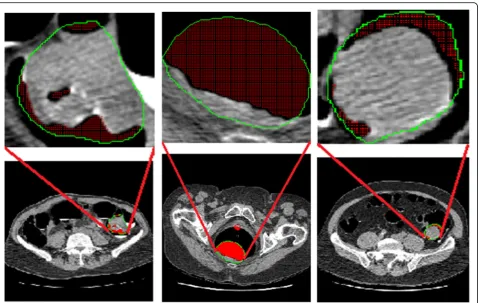
Tumor heterogeneity describes the observation that dif-ferent tumor cells can show distinct morphological and phenotypic profiles. It has become a critical measure in benign and malignant differentiability. The lesion’s hetero-geneity is closely related to the lesion image textures (Fig.1). However, texture pattern extraction remains a great challenge [10–14]. The method proposed by Haralick et al. [15], the gray-level co-occurrence matrix (GLCM)-based texture descriptor, is identified as a promising solution for this problem. GLCM-based textures have been a forerunner in this field and adapted to multiple diseases such as polyps, breast cancer, lung nodules, gliomas, bladder cancer, and imaging modalities including CT, magnetic resonance imaging, positron emission computed tomography [16–19]. In the past, Lam [20] extended gray level co-occurrence matrix (CM) by gradient magnitude to extract image

© The Author(s). 2019Open AccessThis article is distributed under the terms of the Creative Commons Attribution 4.0 International License (http://creativecommons.org/licenses/by/4.0/), which permits unrestricted use, distribution, and reproduction in any medium, provided you give appropriate credit to the original author(s) and the source, provide a link to the Creative Commons license, and indicate if changes were made.

* Correspondence:[email protected]

2_{The Departments of Radiology and Biomedical Engineering, Stony Brook} University, Stony Brook, NY 11794, USA

textures and Guo [21] explored CM by Gaussian curvatures to construct shape descriptors. In the recent years, Song et al. [22] introduced some high order metrics, such as gra-dient magnitude and curvature, to expand Haralick features (HFs) in volumetric data for polyp classification. To further improve the distinctions of the Haralick measures in differ-ent directions, Hu et al. [23] used the Karhunen-Loeve transform (KLT) to map the Haralick measures into an or-thogonal eigenspace.

The Haralick model defines and extracts some im-portant texture patterns from images. These patterns reveal image intensity correlation for pixel pairs on each two-dimensional (2D) image slice. Nevertheless, descriptors computed using the Haralick model in the 2D presentation have certain limitations. The model analyzes the nearest neighboring pixel in four different directions which is described in Section 2. The HFs are often extracted to construct rotational invariant descriptors which are formed by the means and ranges of Haralick measures along those four directions. However, the potential drawbacks of four-directional-averaging in a 2D digital image lack rotational robustness. On the other hand, the traditional Haralick model always counts all pixel pairs and calculates their distribution over all slices by full sampling which could result in redundant

information and weaken the model’s performance. The third shortcoming of the Haralick model is the consider-ation of the nearest neighboring pixel to construct texture features: not considering other displacements may limit the potential to further extract textural patterns.

In this paper, we modify the definition of GLCM by adding a new variable - stride, and introducing multiple scaling analysis into the texture descriptor construction via GLCM. To address the weaknesses of the Haralick model, three schemes associated with each of the vari-ables in GLCM, i.e., displacement, stride and angle, are devised to evaluate the CM-texture descriptors. Each scheme seeks to increase texture patterns through multiple scaling analysis while being mindful of texture information redundancy associated with the learning method. Furthermore, we intend to find out which vari-able would be more sensible in a multi-scale framework. Six classification schemes are designed for our investiga-tion by random forest (RF).

The remainder of this paper is organized as follows: Section 2 describes and reviews the baseline Haralick model and proposes our new adaptive sampling model. Section 3 includes the analysis on the design and the results of our method. The last section includes some discussions and conclusions.

Methods

This section begins with a review of the basic Haralick model in 2D and 3D space. Then, the proposed multiple scaling gray-level co-occurrence model (MSGLCM) is pre-sented. The individual parameters from MSGLCM are each evaluated independently in three learning models, namely by multiple displacements, multiple strides and multiple angles.

2D/3D Haralick model

The Haralick model was proposed to extract polyp texture information from intensity images because of its strong ability to discriminate polyp pathologies [22, 23]. This model’s pipeline includes calculating image metrics such as its intensity, gradient and curvature, etc., image metric digitalization, GLCM computation, Haralick measure and feature definition,

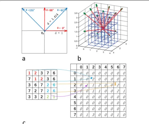
and image descriptor construction. The GLCM com-putation defines and extracts important texture pat-terns (distribution of pixel-pairs) from one image along different directions (Fig. 2).

The method provides 14 measures for every matrix computation. In a 2D gray image, four directions (0°, 45°, 90° and 135°) are analyzed (Fig. 2a). From each dir-ection, one image would generate HFs consisting of 28 texture variables, i.e., 14 means and 14 ranges which would be used to construct the texture descriptor. In contrast, the number of directions in volumetric data is 13 (Fig.2b). Hu et al. [23] expanded this model to gener-ate 30 measures, referred to as the extended Haralick measures (eHM), to capture more texture information from volumetric data. Unlike the Haralick model, they employ all measures to form the texture descriptor in-stead of HFs.

Proposed multi-scaling GLCM model

The proposed method utilizes three primary variables for the multi-scaling model, i.e., displacement scaling, stride scaling, and angle scaling. Using these values, the equation for the multi-scaling GLCM (MSGLCM) can be presented as below:

Ci;jðd;θ;sÞ ¼XMm¼1; m←mþs

XN n¼1 n←nþs

1 I mð ;nÞ ¼i;I mðð ;nÞ þdθÞ ¼j

0 otherwise

ð1Þ

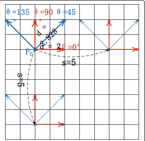
I represents the grayscale image, (M, N) is the image size,iandjare a pair of image pixel values,dis the dis-placement between two pixels along the angle θ, and s represents the stride. A pictorial illustration of Eq. (1) is shown in Fig. 3. When s=d= 1, the MSGLCM should be the traditional GLCM model. This model provides a new tool to capture more texture patterns at multiple scales. A typical example of MSGLCM calculation is shown by Fig. 3 where the stride is equal to 5. The MSGLCM model for 3D volumetric data is similar to the 2D model except that its coefficients are bidirectional.

According to MSGLCM definition, there are three important variables in the learning model, i.e., displace-ments, strides and angles. Each variable would be inves-tigated individually and expanded to larger magnitudes to determine their individual behavior in the model. The following subsections present the methods where each of these three parameters are investigated for the contri-bution to the multi-scaling framework.

Learning model by multiple displacements

The traditional Haralick model has a sampling distance of 1. In medical images, there are more complex textures and using a displacement of 1 might limit the information used to define texture patterns. To evaluate the effect of displacement on the texture pattern, the other two coeffi-cients, i.e., angle and stride, are fixed as follows:

CMD i;jð Þ ¼d

XM m¼1; m←mþ1

XN n¼1; n←nþ1

1 I mð ;nÞ ¼i&I mðð ;nÞ þdθ0Þ ¼j

0 otherwise

ð2Þ

whereθ0∈{(0, 0, 1), (0, 1, 0), (1, 0, 0), (0, 1, 1), (1, 0, 1), (1, 1, 0), (−1, 1, 0), (0, 1, -1), (1, 0, -1), (1, 1, 1), (− 1, 1, 1), (1, 1, -1), (−1, 1, -1)} as shown in Fig.2b.

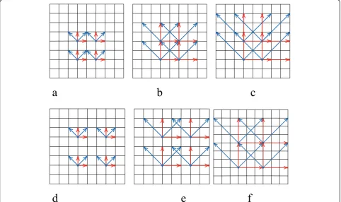
In learning model by multiple displacements (LMD), we adopt an up-sampling method to get more texture patterns. Considering the small volumes of the polyps, large displacements are not ideal while calculating MSGLCM. Smaller displacements, i.e., 1, 2, 3, are used in this exploration study (Fig.4).

The calculation produces three matrix sets for three displacements. Each matrix set contains 13 matrices as-sociated with 13 digital angles [23]. This method gener-ates more texture patterns and texture descriptors for polyp classification compared to the traditional Haralick model.

Learning model by multiple strides

With the increased information that can be extracted with the MSGLCM model compared to the traditional method, the stride can be used as a form of down sam-pling to control multiple scaling implements while cal-culating the CM. Suppose the current position is (x, y); the next position for the model would be (x + stride, y) in the row, or (x, y + stride) in the column. A similar technology can be found in deep learning [24, 25]. In this scheme, stride is the variable which is kept for evaluation while the displacement and angle are con-stants as described by the following equation.

CMS i;jð Þ ¼s

XM m¼1; m←mþs

XN n¼1

n←nþs

1 I mð ;nÞ ¼i;I mðð ;nÞ þd0θ0Þ ¼j

0 otherwise

ð3Þ

whered0is the fixed displacement andθ0has 13 alterna-tives as shown in Formula (2).

This method is similar to LMD with the addition of the stride analysis for the MSGLCM calculation. Unlike displacement, increasing the stride will lead to a down-sampling process. Likewise, smaller strides are consid-ered more ideal for MSGLCM calculation since the sizes of the polyps are always small. The strides that are eval-uated for this method will be limited by the size of the region of interest (ROI) volumes used. The base model Fig. 3Calculation of multi-scale gray level co-occurrence matrix

wheredrepresents displacement,θis the angle,sis stride (or scale),

for this design includes 13 directions and a displacement of 1, though it can be further expanded with LMD to in-crease the displacement and stride. Example cases of using a stride of 2 and 3 are illustrated in Fig.5.

In image classification, the performance is significantly determined by some key features. The traditional full sampling will generate more redundancy while decreas-ing the ratio of key features, which will hurt the cluster-ing performance. This method provides a solution via decreasing the sampling frequency over the image to lessen the number of non-critical features. Therefore, the down-sampling method intends to enhance the roles

of key features in polyp classification to improve the clustering results.

Learning model by multiple angles

Angle sampling rate in a 3D image array can mitigate sparse directions in the model by including higher or-ders of neighbors in CM. The angles in digital images or volume data are discretized and as a result, increasing the digital angles requires more displacements in the digital domain. Similar to the previous designs, i.e., LMD and learning model by multiple strides (LMS), the dis-placements used to evaluate the new design are 1, 2 and Fig. 4MSGLCM calculation by displacement samplings: (a) displacement = 1, (b) displacement = 2, (c) displacement = 3

3 due to concern for polyp size (i.e., 3 mm and larger). The following equation describes the MSGLCM with variable angles and a fixed stride.

CMAi;jð Þ ¼θ

XM m¼1; m←mþ1

XN n¼1;

n←nþ1

1 I mð ;nÞ ¼i&I mðð ;nÞ þθÞ ¼j

0 otherwise

ð4Þ

whereθis the digital angle represented by some 3D vec-tors similar to Formula (2).

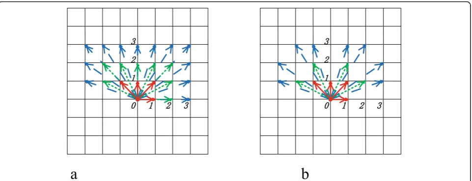
It is easy to see this is an up-sampling model similar to LMD. Furthermore, LMD is a subset of learning model by multiple angles (LMA). Each displacement could generate a set of angles (Fig.6a). The angles of dif-ferent displacements are listed in Table 1. To examine the behavior of multiple angles, the displacement and the stride will be set as 1 for the base model. Further ob-servation will include increasing the displacement and increasing the stride. Note that some angles in digital images can be duplicated as we include more directions while increasing displacements (Fig. 6a). To investigate the impact of these repeated angles in polyp classifica-tion, they are removed in another scheme, as shown in Fig.6b.

All the proposed models could be able to generate new texture information different from the traditional Haralick model via multi-scaling on displacements, strides and angles. However, with the increased pool of information, the texture patterns would bring not only more useful information but also some redundancies. This can potentially lead to overfitting problems in polyp categorization which could lower the clustering perform-ance and consequentially hurt the classification. There are numerous debates on this topic which could be solved by appropriate feature selection methods [26–28].

Polyp descriptors and classifier

Polyp descriptors

Polyp descriptors are numeric descriptions in the form of scalars, vectors, or matrices that describe a polyp ex-tracted from a polyp image or volume. In this article, the eHM are utilized to construct the polyp descriptors [23]. For MSGCLM, eHM defines 30 measures that expands the 14 traditional Haralick measures with 16 new mea-sures. However, the 21th measure which represents clus-ter average is always equal to 0, and the 25th and 30th measures are equivalent after formula simplification. Therefore, the descriptor will include 28 measures for one direction. For multiple angles, the vector will have N * 28 variables to represent a polyp where N is the angle number.

Classifier and feature selection

Classification is one of the most effective tools for iden-tifying descriptors. Its major task is to identify general patterns belonging to one category. The simplest case is binary classification which creates a function g:x→{1,

−1}, wheregis a classifier [29].

RF classification is derived from a decision tree (DT) method [30]. Unlike DT, RF will apply many trees to train and test the samples, then a voting method is used to get the probability from these trees. Another distinc-tion is the random sampling in the tree construcdistinc-tion that includes randomly splitting features, combinations

Fig. 6Two cases of multiple angle sampling: (a) multiple angle sampling with duplicates, (b) multiple angle sampling without duplicates Table 1Angle groups of two cases in Fig.6under three different displacements

Angles Displacement Displacement Displacement

≤1 ≤2 ≤3

With duplicates 13 62 171

of features and choosing the threshold. For each process of RF, the descriptors of all polyps are divided into train-ing groups and testtrain-ing groups. Before classification, we first calculate the priority of each variable in the texture descriptor. GINI coefficient is introduced to be the pri-ority measurement in our method. Then some variable sets are generated using the forward step feature selec-tion method on the ranked variables [23,31]. Thereafter, classifications are performed on each variable set under the parameter of 2000 trees and pffiffiffiffiffiffiffiffiffiffiffiffiN28 candidate vari-able number. We utilize the area under the curve of receiver operating characteristics (AUC) to be our evalu-ation measurement. The feature set with the highest AUC score would be taken to be the optimized texture descriptor.

Some operations for volume of interests and digital angles

Before differentiating the types of polyps, each polyp’s position (x, y, z) in a volumetric data was labelled by radiologist experts. Next, a semiautomatic performance is adopted to crop the polyp patches on every image slice. For that purpose, the labeled polyps are outlined manually to generate ROIs on all slices according to the labelled location. The polyp locations are continuous: lo-cated on every slice and form a volume of interest (VOI). Due to the manual labelling, the resulting VOIs include additional information such as air. To separate the air from the polyp, an adaptive air-cleansing algo-rithm is employed to eliminate those voxels that contain predominately air [32].

The digital angles are defined in accordance to the grid structure of a digital image. As a result, the distance for each digital angle may not always be integers. To ad-dress this issue, vectors are used to provide information on angle and magnitude which correspond to the angle and displacement in the proposed models.

The traditional GLCM is calculated including the in-verse angles to produce a symmetric matrix. The Hara-lick measures are symmetrically invariant; therefore, the matrix and its symmetric iteration can produce the same measures. To reduce redundant measures, the inverse directions are excluded from the digital angles. Only

four angles are included in the 2D Haralick model corre-sponding to (1, 0), (1, 1), (0, 1), and (1, −1). Similarly, the extended Haralick model in 3D would include more directions with the increase of the displacement.

Results Polyp dataset

A private dataset containing 59 patients with a total number of 63 polyp masses is used for the experiments of this study. All the polyp masses are at least 30 mm in diameter. Each polyp was identified by radiologist ex-perts on CTC and optical colonoscopy. All the patients were scheduled for surgical removal intervention after detection and confirmation. When the polyp masses were removed, all pathology reports were obtained to verify whether each of the polyp masses was indeed a cancerous (adenocarcinoma) or benign (adenomatous) polyp. The breakdown of the dataset can be seen in Table 2. To benefit surgical intervention, it is important to know the malignant risk of each polyp mass. Given the pathology reports, these polyp CTC scans provide an excellent database to develop machine learning strategies to predict adenocarcinoma for more aggressive removals. In addition to direct clinical impact, this database also provides good opportunities to evaluate different ma-chine learning strategies regarding to pathological ground truth. This study is an example of evaluating methodology development for polyp classification using the pathologically approved database.

Classification needs two sub-datasets, the training dataset and the testing dataset. From the polyp mass database, we randomly selected 15 samples from the be-nign polyps and 16 from the malignant polyps for train-ing. The remaining polyps are used for testtrain-ing. Thus 31 polyps are used for training and 32 for testing (Table 3). Repeating the random sampling method, we generated 100 unique iterations for training and testing groups.

Experimental outcomes

According to the three multi-scale models, six testing schemes are designed. We test the three models sep-arately. Then three hybrid experiments are designed and implemented.

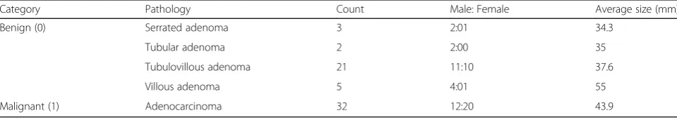
Table 2Polyp masses dataset used for experiments

Category Pathology Count Male: Female Average size (mm)

Benign (0) Serrated adenoma 3 2:01 34.3

Tubular adenoma 2 2:00 35

Tubulovillous adenoma 21 11:10 37.6

Villous adenoma 5 4:01 55

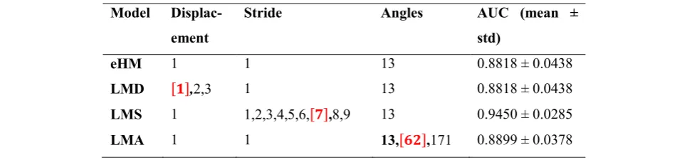
Results of LMD, LMS and LMA

To calculate LMD, the displacements vary between {1, 2, 3} while its stride remains constant at 1 and with 13 an-gles. As we test LMS, its strides vary in {1, 2, 3, 4, 5, 6, 7, 8, 9}. Its displacement remains 1 and 13 angles are in-volved in the calculation. For LMA, both its displace-ment and stride stay 1 while the total angles are set as {13, 62, 171}. After classification, their AUC scores are listed in Table 4. Their results tell us that the stride is more effective to improve the descriptor distinction than the other two parameters of displacement and angle since its AUC score is improved by about 6%. Compared with eHM (baseline), the LMD and LMA are almost even and do not bring much gain for polyp classification when we change the displacement and the angle num-bers independently.

Hybrid results of LMD + LMS

In this experiment, LMD and LMS are combined to ex-tract some new texture patterns. There are 3 different dis-placements and 9 strides involved in texture descriptor construction. Hence, 27 kinds of polyp descriptors are generated. The number of angles is kept constant with 13 directions. After training and testing via RF, their AUC scores are calculated and illustrated in Table5. It retells us that the stride is more sensitive than the displacement. With the stride increasing, we see that the classification performance generally increases in a staggering fashion. However, the trend of AUC scores on each row are grad-ually declining while the displacement is growing which

means LMD introduces more redundant information for polyp classification.

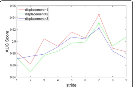
From these results, there is an increasing trend with odd strides as the stride approaches 7. Similar outcomes are reached with the increasing displacements. These outcomes demonstrate that the LMA model with a larger stride could produce more critical features and get much better performance for polyp classification. Figure 7 is plotted to illustrate the AUC score changes according to stride and displacement.

Hybrid results of LMS + LMA

In this experimental scheme, we try to combine LMS and LMA to investigate the second hybrid model with three parameters. The angle sampling method in Fig. 6 shows that more digital angles need more displacements which determines the digital angle number under full sampling. That means angle group and displacement ex-ists in a one-to-one relationship under a full sampling scheme in digital images. Therefore, this type of hybrid model contains two parameters, i.e., angle number and strides. Moreover, the previous schemes indicate that the displacement does not obtain any benefit, while the stride produced significant impact on the AUC score. Therefore, the following scheme keeps 3 displacements while the stride varies from one to nine. The results of the scheme with duplicate angles are described in Table6 and the scheme without duplicate angles is described in Table7.

The best performing model follows the same conven-tion from the previous model with an AUC of 0.9450 for angle = 13 and S = 7. However, the average AUC tells us that this angle group is not stable with the stride varying, as shown in Tables6 and 7. Considering the stability of the model, the group with 62 angles shows some advan-tages over others. Its averaged AUC score reaches 90.55% with the smallest standard deviation 0.0378. The results of 62 angles also indicate that the 1st and 2nd nearest neighbors contain more distinctive texture descriptors while the third nearest neighbor brings Table 3The training samples and testing samples for polyp

classification

Dataset Total Category Number

Training 31 Benign 15

Malignant 16

Testing 32 Benign 16

Malignant 16

Table 4The OCR for LMD, LMS and LMA

redundant information which hurts the classification performance to a small extent. Compared to the first row in Table5, the AUC scores improved about 1%–2% with increasing directions. The multi-stride continues enhancing this criterion to 94% when s = 7.

Comparisons

To illustrate the efficiency of our method, some typical methods are introduced to compare with our models. These methods are listed as the following.

HF–a typical method was proposed to construct the texture descriptor consisting of 28 HFs extracting from CM [15].

eHM – a new model introduced 30 measures to represent texture characteristics extracted from CM [23].

K-L transform based eHM (eHM + KLT)–this method introduced K-L transform to enhance the distinction between two different image features and reduce variation [23].

Co-occurrence of local anisotropic gradient orientation (CoLIAGe)–this model employed gradient angles and extracted the entropy of every local patch to form a global texture descriptor by two joint histograms [33].

VGG16–this method extracts 20 salient slices from every polyp volume to feed to VGG16 for polyp classification [34].

We choose two results from two hybrid results of our method for this comparison, i.e., LMD + LMS with stride = 7 and D = 1, LMS + LMA with angles = 62 and stride = 7. Their receiver operating characteristic curves are plotted in Fig.8 which illustrates their different per-formances for polyp classification. Moreover, their AUC Table 5AUC scores of three CM sets with nine different strides

for LMD + LMS where D represents displacement

D = 1 D = 2 D = 3

S = 1 0.8818 ± 0.0438 0.8725 ± 0.0461 0.8706 ± 0.0489

S = 2 0.8621 ± 0.0487 0.8486 ± 0.0458 0.8751 ± 0.0477

S = 3 0.9043 ± 0.0382 0.8765 ± 0.0407 0.8786 ± 0.0463

S = 4 0.8919 ± 0.0382 0.8834 ± 0.0368 0.8907 ± 0.0417

S = 5 0.9159 ± 0.0408 0.8971 ± 0.0443 09073 ± 0.0446

S = 6 0.9057 ± 0.0394 0.8988 ± 0.0400 09042 ± 0.0447

S = 7 0.9450 ± 0.0285 0.9303 ± 0.0393 0.9223 ± 0.0375

S = 8 0.8887 ± 0.0366 0.8924 ± 0.0436 0.8838 ± 0.0397

S = 9 08825 ± 0.0452 0.9073 ± 0.0421 0.8714 ± 0.0402

Average 0.8975 ± 0.0.399 0.8896 ± 0.0421 0.8893 ± 0.0435

AUCArea under the curve of receiver operating characteristic curve,CM Co-occurrence matrix,LMSLearning model by multiple strides,LMDLearning model by multiple displacements

Fig. 7AUC score trends with the stride increasing for LMD + LMS. “*”indicates the best result position of each curve. AUC: Area under the curve of receiver operating characteristic curve; LMS: Learning model by multiple strides; LMD: Learning model by

multiple displacements

Table 6AUC scores of LMA with duplicates angles over 100 training and testing groups

Angles = 13 Angles = 62 Angles = 171

S = 1 0.8818 ± 0.0438 0.8899 ± 0.0378 0.8887 ± 0.0377

S = 2 0.8621 ± 0.0487 0.8527 ± 0.0463 0.8561 ± 0.0512

S = 3 0.9043 ± 0.0382 0.9053 ± 0.0387 0.9055 ± 0.0374

S = 4 0.8919 ± 0.0382 0.9075 ± 0.0369 0.8993 ± 0.0354

S = 5 0.9159 ± 0.0408 0.9211 ± 0.0385 0.9246 ± 0.0347

S = 6 0.9057 ± 0.0394 0.90764 ± 0.0364 0.9093 ± 0.0392

S = 7 0.9450 ± 0.0285 0.9457 ± 0.0293 0.9378 ± 0.0304

S = 8 0.8887 ± 0.0366 0.9004 ± 0.0373 0.8959 ± 0.0371

S = 9 08825 ± 0.0452 0.9194 ± 0.0391 0.9187 ± 0.0435

Average 0.8975 ± 0.0399 0.9055 ± 0.0378 0.9039 ± 0.0385

AUCArea under the curve of receiver operating characteristic curve,LMA

Learning model by multiple angles

Table 7AUC scores of LMA without duplicate angles over 100 training and testing groups

Angles = 13 Angles = 49 Angles = 145

S = 1 0.8818 ± 0.0438 0.8833 ± 0.0387 0.8926 ± 0.0383

S = 2 0.8621 ± 0.0487 0.8524 ± 0.0512 0.8515 ± 0.0499

S = 3 0.9043 ± 0.0382 0.9054 ± 0.0388 0.9062 ± 0.0387

S = 4 0.8919 ± 0.0382 0.9084 ± 0.0376 0.8918 ± 0.0385

S = 5 0.9159 ± 0.0408 0.9176 ± 0.0337 0.9263 ± 0.0369

S = 6 0.9057 ± 0.0394 0.9077 ± 0.0377 0.9121 ± 0.0383

S = 7 0.9450 ± 0.0285 0.9401 ± 0.0319 0.9388 ± 0.0285

S = 8 0.8887 ± 0.0366 0.8962 ± 0.0335 0.8939 ± 0.0362

S = 9 08825 ± 0.0452 0.9226 ± 0.0364 0.9202 ± 0.0384

Average 0.8975 ± 0.0399 0.9037 ± 0.0377 0.9037 ± 0.0382

AUCArea under the curve of receiver operating characteristic curve,LMA

scores, accuracies, sensitivities and specificities are also listed in Table 8 for further evaluation. To verify their differences, P-values are calculated using t-test to deter-mine if our method is significantly different from others, as shown in Table 9. All the P-values are far smaller than 0.05 which indicates that the proposed methods are distinctive to all the typical methods.

Conclusions

This paper reviews the properties and evaluates the po-tential of the Haralick model by examining several weak-nesses observed in practice [22, 23]. The multi-scale gray level co-occurrence matrix (MSGLCM) is proposed and aims to improve this model by incorporating the multi-scale analysis technique with GLCM to evaluate the three variables: displacement, stride, and angular di-rections. MSGLCM combines the stride and

down-sampling technology to emphasize the unique features and lessen the number of non-critical characteristics to improve polyp classification performance. Meanwhile, MSGLCM adopts up-sampling techniques to integrate the displacement and angle to get new texture patterns which could mitigate the sparse sampling problem within the GLCM calculation. With the increase of tex-ture patterns and textex-ture descriptors, the forward step feature selection method is applied to solve the inform-ative redundancy and overfitting issues in polyp classifi-cation over 63 polyp masses: including 32 invasive adenocarcinomas and 31 benign adenomas.

Experimental results reveal that increasing stride can significantly improve polyp classification over the trad-itional HF and eHM. On the other hand, displacement has little if any positive effect on the results on its own. With the addition of increasing displacements whilst preserving the lower displacements, there were varying results which demonstrates that there can be potential gains in additional displacements. This proposed model can achieve higher AUC values compared to the typical methods discussed in section 3.3. The best model from our experiments had a 6.23% improvement and reduced the standard deviation by 34.95% which is a significant advantage over them.

Discussion

Why the stride is more sensitive than the displacement and angle is still a question for us. The reasons might be guessed from two aspects. The type of polyp texture might be the first reason. The polyp texture should be-long to one type of stochastic texture which has no ap-parent textural structures [35–37]. This type of texture is not sensitive to the changes of directions and displace-ment because of its isotropy. The second reason might be informative redundancy introduced by multiple an-gles on stochastic texture. The multi-angle sampling produced too many similar texture patterns from polyps. Since the classification and recognition should depend on some unique features which should play a key role in it, these unique features always make up a very small proportion in the whole feature space [38]. The trad-itional full-sampling or up-sampling technique makes its proportion much smaller. The stride seems to lessen the Fig. 8Receiver operating characteristic curves of six methods via

random forest except VGG16. HF: Haralick feature; eHM: Extended Haralick measure; KLT: Karhunen-Loeve transform; LMD: Learning model by multiple displacements; LMS: Learning model by multiple strides; LMA: Learning model by multiple angles; CoLIAGe: Co-occurrence of local anisotropic gradient orientations

Table 8Four evaluation measurements for seven methods

Method AUC Accuracy Specificity Sensitivity

HF 0.8751 0.8151 0.8093 0.7693

eHM 0.8863 0.8363 0.8281 0.7256

eHM + KLT 0.9073 0.8873 0.8812 0.8475

CoLIAGe 0.9229 0.8835 0.8393 0.8331

VGG16 0.8234 0.8404 0.8069 0.8066

LMD + LMS 0.9449 0.8934 0.9019 0.8851

LMS + LMA 0.9447 0.8915 0.8801 0.9031

HFHaralick feature,eHMExtended Haralick measure,KLTKarhunen-Loeve transform,LMDLearning model by multiple displacements,LMSLearning model by multiple strides,LMALearning model by multiple angles,CoLIAGe

Co-occurrence of local anisotropic gradient orientations,AUCArea under the curve of receiver operating characteristic curve

Table 9Wilcoxon signed-rank test between AUC scores of our methods and the typical methods

Our method HF eHM eHM + KL CoLIAGe VGG16

LMD + LMS << 0.05 << 0.05 << 0.05 << 0.05 << 0.05

LMS + LMA << 0.05 << 0.05 << 0.05 << 0.05 << 0.05

HFHaralick feature,eHMExtended Haralick measure,KLTKarhunen-Loeve transform,LMDLearning model by multiple displacements,LMSLearning model by multiple strides,LMALearning model by multiple angles,CoLIAGe

non-critical texture patterns and improve the ratio of unique features while down-sampling. We found that the higher sampling rate from a low stride may drown out those texture patterns that are necessary for distin-guishing between pathologies.

In summary, our proposed model has shown encour-aging performance. Nevertheless, redundant information and over-fitting issues by descriptor variables still face great challenges which need new feature selection tech-nologies to solve. Further investigation is required in implementing convolutional neural networks to solve polyp classification on a small database [25]. Both of these are important tasks for our research efforts in the future.

Abbreviations

2D:Two-dimensional; AUC: Area under the curve of receiver operating characteristic curve; CADx: Computer-aided diagnosis; CM: Co-occurrence matrix; CoLIAGe: Co-occurrence of local anisotropic gradient orientations; CRC: Colorectal carcinoma; CTC: Computed tomographic colonography; DT: Decision tree; eHM: Extended Haralick measure; GLCM: Gray-level co-occurrence matrix; HF: Haralick feature; KLT: Karhunen-Loeve transform; LMA: Learning model by multiple angles; LMD: Learning model by multiple displacements; LMS: Learning model by multiple strides; MSGLCM: Multi-scaling gray-level co-occurrence model; OC: Optical colonoscopy; RF: Random forest; ROIs: Regions of interest; VOI: Volume of Interest

Acknowledgments

The authors would appreciate the editing efforts from Mr. Kenneth Ng and Ms. Anushka Banerjee.

Authors’contributions

All authors discussed the major idea and the details of this article. They all read and approved the final manuscript.

Funding

This work was supported by the NIH/NCI, No. CA206171.

Availability of data and materials

All experiments are performed on a private database of IRIS (Imaging Research and Informatics) Laboratory, State University of New York at Stony Brook.

Competing interests

The authors declare that they have no competing interests.

Author details

1

The Department of Radiology, Stony Brook University, Stony Brook, NY 11794, USA.2_{The Departments of Radiology and Biomedical Engineering,} Stony Brook University, Stony Brook, NY 11794, USA.3_{The Department of} Radiology, School of Medicine, University of Wisconsin, Madison, WI 53792, USA.

Received: 26 August 2019 Accepted: 12 November 2019

References

1. American Cancer Society (2018) Cancer facts & figures 2018. American Cancer Society, Atlanta, GA, USA

2. Byers T, Levin B, Rothenberger D, Dodd GD, Smith RA (1997) American Cancer Society guidelines for screening and surveillance for early detection of colorectal polyps and cancer: update 1997. CA: A Cancer J Clin 47(3):154_– 160https://doi.org/10.3322/canjclin.47.3.154

3. Levin B, Lieberman DA, McFarland B, Smith RA, Brooks D, Andrews KS et al (2008) Screening and surveillance for the early detection of colorectal cancer and adenomatous polyps, 2008: a joint guideline from the American Cancer Society, the US multi-society task force on colorectal cancer, and the

American college of radiology. CA: A Cancer J Clin 58(3):130–160https://doi. org/10.3322/CA.2007.0018

4. Center MM, Jemal A, Smith RA, Ward E (2009) Worldwide variations in colorectal cancer. CA: A Cancer J Clin 59(6):366–378https://doi.org/10.3322/ caac.20038

5. Liang ZR, Richards R (2010) Virtual colonoscopy vs optical colonoscopy. Expert Opin Med Diagn 4(2):159–169https://doi.org/10.1517/ 17530051003658736

6. Pickhardt PJ (2013) Missed lesions at CT colonography: lessons learned. Abdom Imaging 38(1):82–97https://doi.org/10.1007/s00261-012-9897-z 7. Rathore S, Hussain M, Ali A, Khan A (2013) A recent survey on colon cancer

detection techniques. IEEE/ACM Trans Comput Biol Bioinform 10(3):545_–563 https://doi.org/10.1109/TCBB.2013.84

8. Ma M, Wang HF, Song BW, Hu YF, Gu XF, Liang ZR, et al (2014) Random forest based computer-aided detection of polyps in CT colonography. In: abstracts of 2014 IEEE nuclear science symposium and medical imaging conference, Seattle, 8-15 November 2014

9. Song BW, Zhang GP, Zhu W, Liang ZR (2014) ROC operating point selection for classification of imbalanced data with application to computer-aided polyp detection in CT colonography. Int J Comput Assist Radiol Surg 9(1): 79–89https://doi.org/10.1007/s11548-013-0913-8

10. Castellano G, Bonilha L, Li LM, Cendes F (2004) Texture analysis of medical images. Clin Radiol 59(12):1061–1069https://doi.org/10.1016/j. crad.2004.07.008

11. Fiori M, Musé P, Aguirre S, Sapiro G (2010) Automatic colon polyp flagging via geometric and texture features. In: Abstracts of 2010 annual international conference of the IEEE engineering in medicine and biology, Buenos Aires, 31 August-4 September 2010.https://doi.org/10.1109/IEMBS. 2010.5627185

12. Cao W, Pomeroy MJ, Pickhardt PJ, Barish MA, Stanly S III, Liang Z (2019) A local geometrical metric-based model for polyp classification. In: Mori K, Hahn HK (eds) Proceedings of SPIE Medical Imaging, San Diego, 2019. https://doi.org/10.1117/12.2513056

13. X. Hong, G. Zhao, M. Pietikäinen, and X. Chen,“Combining LBP Difference and Feature Correlation for Texture Description,_”IEEE Transactions on Image Processing, vol. 23, no. 6, pp. 2557-2568, 2014.

14. Rathore S, Hussain M, Iftikhar MA, Jalil A (2014) Ensemble classification of colon biopsy images based on information rich hybrid features. Comput Biol Med 47:76–92https://doi.org/10.1016/j.compbiomed.2013.12.010 15. Haralick RM, Shanmugam K, Dinstein IH (1973) Textural features for image

classification. IEEE Trans System Man Cybernet SMC-3(6):610_–621https://doi. org/10.1109/TSMC.1973.4309314

16. Rangayyan RM, Nguyen TM, Ayres FJ, Nandi AK (2010) Effect of pixel resolution on texture features of breast masses in mammograms. J Digit Imaging 23(5):547–553https://doi.org/10.1007/s10278-009-9238-0 17. Ahmed A, Gibbs P, Pickles M, Turnbull L (2013) Texture analysis in

assessment and prediction of chemotherapy response in breast cancer. J Magn Reson Imaging 38(1):89–101https://doi.org/10.1002/jmri.23971 18. Lee J, Jain R, Khalil K, Griffith B, Bosca R, Rao G, et al (2016) Texture feature

ratios from relative CBV maps of perfusion MRI are associated with patient survival in glioblastoma. AJNR Am J Neuroradiol 37(1):37–43.https://doi.org/ 10.3174/ajnr. A4534

19. Xu XP, Zhang X, Tian Q, Wang HJ, Cui LB, Li SR et al (2019) Quantitative identification of nonmuscle-invasive and muscle-invasive bladder carcinomas: a multiparametric MRI radiomics analysis. J Magn Reson Imaging 49(5):1489–1498https://doi.org/10.1002/jmri.26327

20. Lam SWC (1996) Texture feature extraction using gray level gradient based co-occurence matrix. In: abstracts of IEEE international conference on systems, man and cybernetics, Beijing, 14-17 October 1996 21. Guo KH (2010) 3D shape representation using gaussian curvature

co-occurrence matrix. In: Wang FL, Deng HP, Gao Y, Lei JS (eds) Artificial intelligence and computational intelligence. International conference artificial intelligence and computational intelligence, October 2010. Lecture notes in computer science (lecture notes in artificial intelligence), vol 6319. Springer, Heidelberg, pp 373–380https://doi.org/10.1007/978-3-642-16530-6_44 22. Song BW, Zhang GP, Lu HB, Wang HF, Zhu W, Pickhardt PJ et al (2014)

Volumetric texture features from higher-order images for diagnosis of colon lesions via CT colonography. Int J Comput Assist Radiol Surg 9(6):1021–1031 https://doi.org/10.1007/s11548-014-0991-2

tomography colonography. IEEE Trans Med Imaging 35(6):1522–1531 https://doi.org/10.1109/TMI.2016.2518958

24. LeCun Y, Bengio Y, Hinton G (2015) Deep learning. Nature 521(7553):436– 444https://doi.org/10.1038/nature14539

25. Wainberg M, Merico D, Delong A, Frey BJ (2018) Deep learning in biomedicine. Nat Biotechnol 36(9):829_–838https://doi.org/10.1038/nbt.4233 26. Auffarth B, López M, Cerquides J (2010) Comparison of redundancy and

relevance measures for feature selection in tissue classification of CT images. In: Perner P (ed) Advances in data mining. Applications and theoretical aspects. 10th industrial conference, July 2010. Lecture notes in computer science (lecture notes in artificial intelligence), vol 6171. Springer, Heidelberg, pp 248–262https://doi.org/10.1007/978-3-642-14400-4_20 27. Hawkins DM (2004) The problem of overfitting. J Chem Inf Comput Sci

44(1):1_–12https://doi.org/10.1021/ci0342472

28. Boucheron S, Bousquet O, Lugosi G (2005) Theory of classification: a survey of some recent advances. ESAIM: Probab Stat 9:323–375https://doi.org/10. 1051/ps:2005018

29. Raschka S, Mirjalili V (2017) Python machine learning, 2nd edn. Packt Publishing, Birmingham, UK

30. Breiman L (2001) Random forests. Mach Learn 45(1):5–32https://doi.org/10. 1023/A:1010933404324

31. Zhang ZH (2016) Variable selection with stepwise and best subset approaches. Ann Transl Med 4(7):136https://doi.org/10.21037/atm. 2016.03.35

32. Li X, Li LH, Lu HB, Liang ZR (2005) Partial volume segmentation of brain magnetic resonance images based on maximum a posteriori probability. Med Phys 32(7):2337–2345https://doi.org/10.1118/1.1944912

33. Prasanna P, Tiwari P, Madabhushi A (2016) Co-occurrence of local anisotropic gradient orientations (CoLlAGe): a new radiomics descriptor. Sci Rep 6:37241https://doi.org/10.1038/srep37241

34. Simonyan K, Zisserman A (2014) Very deep convolutional networks for large-scale image recognition. arXiv:1409.1556

35. Efros A, Leung TK (1999) Texture synthesis by non-parametric sampling. In: abstracts of the seventh IEEE international conference on computer vision, Kerkyra, 20-27 September 1999.https://doi.org/10.1109/ICCV.1999.790383 36. Lin WC, Hays J, Wu CY, Kwatra V, Liu YX (2004) A comparison study of four

texture synthesis algorithms on near-regular textures. In: abstracts of SIGGRAPH '04 ACM SIGGRAPH 2004, Los Angeles, 8-12 august 2004.https:// doi.org/10.1145/1186415.1186435

37. Zachevsky I, Zeevi YYJ (2016) Statistics of natural stochastic textures and their application in image denoising. IEEE Trans Image Process 25(5):2130– 2145https://doi.org/10.1109/TIP.2016.2539689

38. Bins J, Draper BA (2001) Feature selection from huge feature sets. In: abstracts of the eighth IEEE international conference on computer, Vancouver, 7-14 July 2001.https://doi.org/10.1109/ICCV.2001.937619

Publisher’s Note