Optimized statistical parametric mapping procedure for NIRS
data contaminated by motion artifacts
Neurometric analysis of body schema extension
Satoshi Suzuki
Received: 3 February 2016 / Accepted: 20 July 2017 / Published online: 29 July 2017 The Author(s) 2017. This article is an open access publication
Abstract This study investigated the spatial distribution of
brain activity on body schema (BS) modification induced by natural body motion using two versions of a hand-tracing task. In Task 1, participants traced Japanese Hira-gana characters using the right forefinger, requiring no BS expansion. In Task 2, participants performed the tracing task with a long stick, requiring BS expansion. Spatial distribution was analyzed using general linear model (GLM)-based statistical parametric mapping of near-in-frared spectroscopy data contaminated with motion arti-facts caused by the hand-tracing task. Three methods were utilized in series to counter the artifacts, and optimal conditions and modifications were investigated: a model-free method (Step 1), a convolution matrix method (Step 2), and a boxcar-function-based Gaussian convolution method (Step 3). The results revealed four methodological findings: (1) Deoxyhemoglobin was suitable for the GLM because both Akaike information criterion and the variance against the averaged hemodynamic response function were smaller than for other signals, (2) a high-pass filter with a cutoff frequency of .014 Hz was effective, (3) the hemo-dynamic response function computed from a Gaussian kernel function and its first- and second-derivative terms should be included in the GLM model, and (4) correction of non-autocorrelation and use of effective degrees of
freedom were critical. Investigating z-maps computed
according to these guidelines revealed that contiguous areas of BA7–BA40–BA21 in the right hemisphere became
significantly activated (tð15Þ;p\:001, p\:01, and
p\:001, respectively) during BS modification while
per-forming the hand-tracing task.
Keywords Body schemaNear-infrared spectroscopy
General linear model Statistical parametric mapping
Hand-tracing task Motion artifacts
1 Introduction
In the human brain, peri-personal space [1] is represented by embedding the spatial volume of external objects, such as a hat (clothing) or a stick (tool), into an internal body map [2]. In this process, people typically feel the object as an extension of their own body [3]. The mechanism underlying this sophisticated cognitive process is known as body schema (BS) modification [4]. This mechanism is considered a form of homuncular flexibility, involving constant changes to the shape of the homunculus, which is an approximate internal map of the human body in the cortex that is often visualized as a distorted human body [5]. The concept of the BS was initially proposed by Head and Holmes [6], who defined it as a postural model of the body that actively organizes and modifies the impres-sions produced by incoming sensory impulses [6]. The existence of the BS was confirmed in the 1990s by ana-lyzing brain function in macaque monkeys [7]. The BS is considered to be vital for spatial cognitive function and is associated with various brain areas, including the sensori-motor cortex [8], Broca’s area (BA44), the inferior parietal lobule (BA40) [9], the primary motor cortex (BA4) [10], and the mirror neuron system [11]. One experimental approach to examining the BS involves the induction of a ‘‘confused’’ brain state by presenting mismatching visual and haptic stimuli, as in the rubber hand illusion S. Suzuki (&)
Department of Robotics and Mechatronics, Tokyo Denki University, 5 Asahi-Chou, Senju, Adachi-ku, Tokyo 120-8551, Japan
(RHI) [12,13]. Similar variations, such as the visual–pro-prioceptive synchrony judgment task [14] and the visual– proprioceptive mismatch task [15], have also been exam-ined. Other studies utilized motion illusions to examine the BS more directly. Motion illusions arise when somatic sensations are confused by physically vibrating the muscle spindle that provides axial and limb position information to the central nervous system [16]. Examples include illusory arm movement [17], the Pinocchio illusion [18], and the waist-shrinking illusion [19]. Electrical stimuli applied to the skin can also induce similar motion illusions [20].
In addition, the BS plays a significant role in the ability to drive a vehicle [21]. For example, a person’s sense of car width is a form of BS modification [22]. For a skilled driver, the whole spatial volume of the vehicle body is perceived as an extension of the driver’s peri-personal space [23]. Such spatial cognitive function is also involved in teleoperation systems that require the operator to manipulate a machine remotely [24]. In both driving a car and remote operation of a robot, the machine (car or robot) must be manipulated like one’s own body. This sensation
of body ownership is a type of BS modification [25,26].
Additionally, the BS is heavily involved in some cog-nitive disorders [27]. Alice in Wonderland syndrome (in-volving distorted awareness of body size, mass, or its position in space), autotopagnosia (involving mislocaliza-tion of body parts and bodily sensamislocaliza-tions), and phantom sensation (awareness of an amputated limb) are examples of such disorders. Because the BS is related to such varied human functions, a quantitative method for evaluating the strength of BS modification may be useful both for reha-bilitation of spatial cognition disorders and for the esti-mation of spatial cognitive skill during vehicle operation. Possible BS measurement methods such as functional magnetic resonance imaging (fMRI), positron emission tomography (PET), and magnetoencephalography (MEG) are, however, not adequate for evaluation, because they all require the participant’s head to be fixed to a stationary measurement unit mounted on the floor. Natural BS mod-ification is difficult to induce using such stationary mea-surement devices because participants cannot move their bodies freely. Near-infrared spectroscopy (NIRS) is an alternative measurement method in which the measurement unit can be attached to the participant’s head while still permitting head movement. NIRS may thus have useful applications in daily life, and portable NIRS systems have recently been marketed commercially.
While NIRS may be an appropriate measurement tech-nique for measuring brain activity during daily tasks, the relationship between NIRS activity and modifications to the BS is not currently understood. While a brain map of BS modification would be useful, no analysis procedure for constructing a map from NIRS data contaminated by
motion artifacts has been established to date. Even mild motion, such as an arm movement, causes strong artifacts in NIRS data. As such, there are several experimental limitations involved in current NIRS methods: the need for participants to maintain a sitting posture, the restriction of movement to the right upper arm only, the inability to twist one’s head, and the need to avoid conversation, all of which may induce cognition-related brain activity that contaminates NIRS data.
Statistical parametric mapping (SPM) has recently become a popular method for investigating the spatial distribution of brain activity [28] in studies using fMRI and PET. Several studies describing the application of SPM to
NIRS data have been reported [14,29–31]. According to
the SPM procedure, characteristics of brain activity are identified statistically using a general linear model (GLM) [32] to evaluate the accuracy of fit of brain activity against a canonical response pattern of cerebral blood flow. Random effects are then analyzed using the accuracy of fit. Because of the effort expended in recent decades to develop the SPM software package [33], this approach has been established as a standard analysis method for fMRI and PET interpretation. SPM is thus becoming the de facto standard for examining common features in human brain activity. It is widely used for investigating brain functions that relate to a wide brain area.
However, unlike fMRI and PET, various adjustments of experimental design analysis are required in NIRS studies, because of the following issues:
Issue 1 To be analyzed with the GLM, signals must
satisfy the assumption of normal
distribution [32]; however, the actual responses of regional cerebral blood flow (rCBF) are not necessarily normally distributed.
Issue 2 It is difficult to satisfy the GLM assumption of non-autocorrelation of errors, since rCBF is time dependent [14].
Issue 3 It is challenging to distinguish meaningful low-frequency components in rCBF from true noise, such as drift and bias.
These issues have often been implicitly ignored in previ-ous studies because the default parameters of the SPM software were applied without careful consideration [31].
In addition, motion artifacts strongly affect NIRS data when analyzing brain activity that accompanies body motion. As such, consideration of body motion is inevitable because natural body motion is required to combine the visual and haptic senses that are involved in BS. Importantly, ill-conditioned data arising from motion artifact contamination cannot satisfy the requirements of
implicitly required for comparison with the canonical waveform. For this reason, most previous studies of NIRS– SPM have utilized experimental paradigms that prohibit body motion (as in fMRI and MEG studies). As such, these methods cannot be directly used to analyze BS modifica-tion accompanying momodifica-tion artifacts. Overall, the brain areas associated with BS modification induced by sponta-neous body motion have not yet been comprehensively examined in humans, although these mechanisms have been identified in the monkey brain [7], and fragmentary
human evidence has been reported [9,11].
Consequently, existing studies of NIRS–SPM have been unable to use the unique benefit of the NIRS method, which permits movement of the head and body. Therefore, the current study sought to establish a practical NIRS–SPM procedure using a task that requires the control of hand and arm movements. The main aims of this study were as follows:
1. Creating guidelines for using NIRS–SPM to analyze
rCBF accompanied by body motion artifacts.
2. Quantifying the spatial distribution of human brain
activity during BS modification induced by natural and spontaneous body motion.
Concerning the first aim, several conditions and modifi-cations were investigated using the following three steps: Step (1) a model-free method analyzing cerebral blood volume (CBV), Step (2) a convolution matrix method known as the orthodox GLM, and Step (3) a boxcar-function-based Gaussian convolution method.
2 Experiment
2.1 Hand-tracing task
A hand-tracing task was devised to examine differences in brain activity related to BS modification. In this task, participants were instructed to trace the curve of Japanese Hiragana characters that were printed on paper (Task 1) or projected onto a screen (Task 2). In Task 1, participants used the right forefinger to trace the characters. In Task 2, participants used a 1.5-m stick held in the right hand to trace characters that were projected 2.0 m in front of them. Importantly, Task 1 entails the use of the BS of partici-pants’ own body only, whereas Task 2 involves an exten-sion of the BS to the tip of the long stick. During both tasks, participants sat on a chair, and the sitting position was adjusted so that the participant could touch the char-acters with the tip of the finger or stick. The size of pro-jected characters was enlarged in proportion to the distance to the screen to keep the perturbation of hand motion similar in both tasks. To avoid inducing unnecessary brain
activation from environmental light and sound, participants performed the tasks while wearing noise-canceling head-phones inside a tent covered with a curtain. Thirty-second
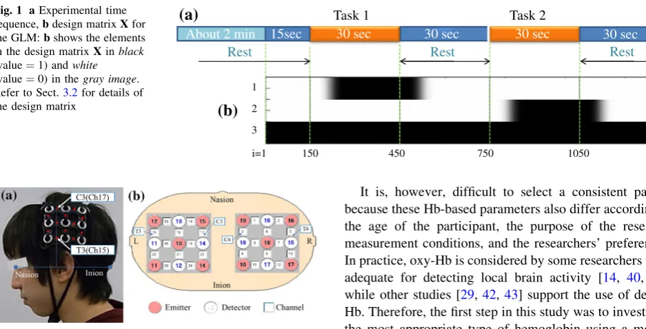
rests were given after each task, as shown in Fig.1a. The
investigator touched the shoulder of the participant to signal the start and end of each task.
2.2 NIRS measurement
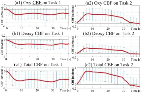
Previous evidence suggests that performing a hand-tracing task would be likely to involve activation in the primary motor area (M1), the primary somatosensory area (S1), and the premotor area (PM) [34–37], because the action involved in hand tracing requires the control of hand and arm movements. The activation of these brain areas alone, however, does not provide sufficient evidence to identify BS modification. Hence, the present study also examined the inferior parietal lobule (BA40). This brain region is not thought to directly relate to hand motion, but is one of the cortical areas associated with BS [9]. Therefore, in the cur-rent experiment, areas around BA40 were monitored using
ETG-4000 (Hitachi Medico, Tokyo, Japan) using two 33
holders, as shown in Fig.2. A total of 24 data channels were
measured. The NIRS probes were attached to participants’ heads using the international 10–20 system so that C3(4) was located at the forefront of the upper array of the holder, and the second vertical line of the holder was perpendicular to the
nasion–inion line, as shown in Fig.2a. Thus, C3(C4) and
T3(T4) on the left (right) hemispheres corresponded to Ch.17(Ch.3) and Ch.15(Ch.5), respectively.
The content and procedure of the experiment were approved by the Tokyo Denki University Human Bioethics Review Committee, and experiments were conducted after explaining the experiment to the participants in full and receiving written consent. Sixteen healthy university
stu-dents (20–23 years old) participated (N¼16) in this
experiment.
3 Analyses
optimal condition for the NIRS–SPM was derived after autocorrelation modification and the final choice of hemoglobin type were identified. These steps fundamen-tally adhere to the following basic stages of a general SPM approach [28]:
First-level analysis
A statistical test ascertains whether the
rCBF shows significantly different
responses according to the task
condition with respect to each
measurement channel (one-samplettest).
Second-level analysis
After statistics obtained in the first-level
analysis are converted into z-values, an
average of the population to which thez
-values of all participants belong is tested (random-effects analysis) [38].
The details of these steps and the analysis results are explained below, in sequence.
3.1 Step 1: Model-free method
The increase of total hemoglobin (Hb) has often been used to investigate brain activity in previous studies. However, other wave patterns such as ‘‘both oxy-Hb and total-Hb decrease’’ and ‘‘oxy-Hb, deoxy-Hb, and total-Hb increase’’ have also been used [39]. In the case of young adults, total-Hb concentration tends to reflect both oxy and deoxy changes, since the increase in oxy-Hb tends to be larger than the decrease in deoxy-Hb [39].
It is, however, difficult to select a consistent pattern because these Hb-based parameters also differ according to the age of the participant, the purpose of the research, measurement conditions, and the researchers’ preferences. In practice, oxy-Hb is considered by some researchers to be
adequate for detecting local brain activity [14, 40, 41],
while other studies [29,42,43] support the use of
deoxy-Hb. Therefore, the first step in this study was to investigate the most appropriate type of hemoglobin using a model-free approach unrelated to the HRF.
Close examination of rCBF responses revealed that regional cerebral blood volume (rCBV) in several channels decreased at the beginning of Task 1 and increased for several seconds at the beginning of Task 2. Based on this observation, a null hypothesis of no difference was tested
using a pairedttest against two values of rCBV, referred to
asS1sandS2s. These values were computed by integrating
the rCBF data for s seconds from the beginning of each
task.
Sls¼
Xs=D
i¼0
ðylðiÞ blÞ=ðs=DÞ ðl¼1;2Þ ð1Þ
bl:¼
X0
i¼b5=Dc
ylðiÞ=ðb5=DcÞ; ð2Þ
whereylðiÞis the rCBF data at the sampling countion Task
lfrom the beginning of the task, the sampling intervalDis
.1 s, bl is a bias computed by averaging 5 s of data just
before the beginning of task, and an operatorbcis a floor
function. The z-values converted from statistics computed
in this pairedttest are shown in Table1. Thez-values were
computed for each channel using all participants’ data
(N¼16), and other results obtained using differentsvalues
are summarized in the same table. This table shows an existence of significant differences in channels 4–10, 12, and 15 for all types of Hb. This result demonstrates that Tasks 1 and 2 induced significantly different brain activity responses.
The current method was a relatively simple process, and
the results shown in Table1may possess lower reliability
because the parameters [an integral intervalsin Eq. (1) and
About 2 min Rest
Task 1
30 sec 30 sec 30 sec
15sec 30 sec
Task 2
Rest Rest
1
2
3
(a)
(b)
i=1 150 450 750 1050 1350 Fig. 1 aExperimental time
sequence,bdesign matrixXfor the GLM:bshows the elements in the design matrixXinblack
(value¼1) andwhite
(value¼0) in thegray image. Refer to Sect.3.2for details of the design matrix
a duration to compute the biasbl in Eq. (2)] were deter-mined subjectively without a theoretical guarantee of optimality, despite consideration of the task condition and the actual NIRS response data. This method, however, contributes to an improved understanding of a tendency in a wide area of common brain activity from multi-channel measurement data. Thus, we assumed the results shown in
Table1 were provisional, and used them to judge the
validity of the assumption of the existence of a certain HRF wave pattern for the subsequent Steps 2 and 3, which were processed from objective criteria. Because the data in this table indicate that the channels responding to the difference between Tasks 1 and 2 were ch. 4–10, 12, and 15, a canonical waveform of rCBF was computed using the rCBF data measured in these channels for the HRF. That is, we averaged all rCBF data measured in these channels during each task period into one waveform for each task.
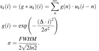
The results of the canonical forms are shown in Fig.3. All
graphs in the figure show rounded trapezoidal waveforms similar to the convolved response of a boxcar and a
Gaussian function. The results revealed that rCBF during Task 1 decreased [see graphs (a1) (b1)] while rCBF during Task 2 increased [see graph (a2) (b2)] for both oxy- and deoxy-Hb. These findings indicated that a waveform sim-ilar to that used in previous studies, involving the con-volved response of a boxcar and a Gaussian function, was appropriate for the current analysis. In addition, the aver-aged rCBF waveform in all cases demonstrated substantial variance because of motion artifacts, as indicated by the long error bars in each graph. Notably, the variance in deoxy-Hb was half that of oxy-Hb [as indicated by the difference in the length of the error bars between graph (a1) and graph (b1), and between graph (a2) and graph (b2)]. This result indicates that deoxy-Hb was less affected by individual differences than oxy-Hb.
Taken together, these findings indicate that deoxy-Hb may be better suited for GLM analysis using the convolved response of a boxcar and a Gaussian function for analysis of rCBF affected by motion artifacts. Therefore, the deoxy-Hb NIRS data were mainly analyzed provisionally in the following analyses. The validity of the selection of deoxy-Hb was judged in Steps 2 and 3.
3.2 Step 2: Convolution matrix method
After Step 1, a GLM–SPM method presented in [44] called the convolution matrix method was applied to the deoxy-Hb responses because the validity of assuming a HRF was confirmed in Step 1, as the procedure presented in [44] is considered a basic version of various extended GLM–SPM methods. To examine differences between the two versions of the hand-tracing task, the following GLM equation was
assumed using independent variables xk ðk¼1;2Þ and a
response variabley.
jyðiÞ ¼ jb
1x1ðiÞ þjb2x2ðiÞ þjdþjeðiÞ; ð3Þ
where jð¼1;. . .;24Þ is an index of channel, bk are
unknown coefficient parameters (const.), d is a drift term
Table 1 Results of statistical tests using a model-free method in Step 1:z-values obtained using a pairedttest,df ¼15
1 2 3 4 5 6 7 8 9 10 11 12 13 14 15 16 17 18 19 20 21 22 23 24 10 2.32 2.12 0.58 3.43 3.15 3.15 3.05 4.11 3.50 3.07 2.01 2.48 1.63 2.26 2.59 0.38 1.66 1.05 1.92 2.18 1.10 0.88 1.80 1.03 20 2.10 1.87 0.21 2.99 3.14 3.22 3.10 4.27 3.14 2.82 2.02 2.86 1.92 1.69 2.57 0.02 1.33 0.30 2.01 2.01 0.83 0.05 1.71 0.59 30 2.05 1.93 0.48 2.75 3.02 3.02 3.00 4.28 2.98 2.81 2.16 2.85 2.07 1.48 2.58 0.30 1.35 0.27 1.86 1.92 0.78 0.27 1.54 0.69 10 2.16 1.81 – 0.90 2.83 2.63 0.89 3.03 1.45 3.32 3.21 1.63 2.88 1.65 2.06 2.35 1.19 – 0.69 2.48 1.29 2.31 0.76 0.89 1.44 0.94 20 2.23 1.36 – 0.96 2.18 2.61 0.04 2.89 1.34 2.97 3.21 1.31 2.82 1.68 1.49 2.12 0.39 0.29 1.27 1.31 2.07 0.53 0.13 1.43 0.76 30 2.10 1.23 –1.00 1.78 2.57 – 0.18 2.71 1.27 2.74 3.18 1.45 2.68 1.63 1.38 1.99 0.68 – 0.15 0.98 1.29 1.98 0.59 0.38 1.35 0.91 10 2.79 2.05 – 0.22 3.41 2.95 3.24 3.15 3.04 3.62 3.31 1.97 2.67 1.83 2.41 2.69 0.67 1.56 1.64 1.73 2.32 1.01 0.91 1.70 1.02 20 2.24 1.71 – 0.39 2.92 2.94 2.26 3.13 2.96 3.22 3.14 1.80 2.91 2.13 1.79 2.61 0.14 1.26 0.56 1.84 2.11 0.74 0.08 1.64 0.66 30 2.19 1.70 – 0.31 2.66 2.86 2.17 2.99 3.03 3.04 3.11 1.95 2.84 2.17 1.57 2.55 0.45 1.27 0.48 1.71 2.02 0.73 0.31 1.51 0.78 Deoxy
Integral interval [s]
Channel number Type
of rCBF
Total Oxy
Blue cells showz[2:33ðp\:01Þ, and red cells showz[3:09ðp\:001Þ. (Color table online)
(a1) Oxy CBF on Task 1 (a2) Oxy CBF on Task 2
(b1) Deoxy CBF on Task 1 (b2) Deoxy CBF on Task 2
(c1) Total CBF on Task 1 (c2) Total CBF on Task 2
0 10 20 30 Time [s]
0 10 20 30 Time [s]
0 10 20 30 Time [s] 0.2
0
-1
CBF [mMmm]
0.2 0
-1
CBF [mMmm]
0.2 0
-1
CBF [mMmm]
0 10 20 30 Time [s] 1
0 -0.2
CBF [mMmm]
0 10 20 30 Time [s] 1
0 -0.2
CBF [mMmm]
0 10 20 30 Time [s] 1
0 -0.2
CBF [mMmm]CBF [mMmm]
(const.), and e is a residual that is assumed to be inde-pendently and identically distributed normally with a
mean of zero. The maximum of the sampling counter i
and the total number of independent variables xk are
denoted as I and K, respectively. Equations defined by
Eq. (3) for all i are summarized in the following matrix
form:
jY¼XjBþjE; ð4Þ
where X2RIðKþ1Þ is a design matrix, Y2RI is a
response vector,B2RðKþ1Þis a parameter vector,E2RI
is a residual vector, andXandBare defined as
X:¼
x1ð1Þ x2ð1Þ 1
.. .
.. .
.. .
x1ðIÞ x2ðIÞ 1 2
6 6 4
3 7 7
5; jB:¼
jb
1
jb
2
jd 2 6 4
3 7
5: ð5Þ
First-level analysis This step investigated whether the hemodynamic responses differed depending on the task conditions by statistically investigating the magnitude of estimations of coefficients in Eq. (3) with respect to each channel for each participant. The details of this technique are explained below.
First, the design matrix X was defined using a
time-series signal of a boxcar function with a value of 1 during the task period and a value of 0 otherwise. Second, a
convolution matrix H2RðIþMÞI was defined using a
Gaussian function to approximate the response of the
rCBF. EstimatesB^forBwere computed as follows, using
the ordinary least squares (OLS) method [44].
jB^¼ XT
aXa
1
XTaHjY
Xa:¼HX
ð6Þ
Specifically, the convolution matrixHwas designed using
a Gaussian function with a 4.0-s full width half maximum
ðFWHM¼4:0Þ[29], and the total length of Ywas
speci-fied as 135 s (i.e., I¼1350) because the data range
including the 15- and 30-s rests at the beginning of Task 1 and the end of Task 2, respectively, was examined, as
shown in previous Fig.1b. Finally, for a statistical test of
the estimates B^, a contrast matrix was chosen as
C¼ ½ 1 1 0, and the Wald statistic (¼CB^/standard
error of slope coefficient) [45] was computed for each
channel and tested with a one-samplet test. Importantly,
the usual degrees of freedom (DoF) used in common GLM
methods computed by ðIrankðXÞÞ[46] are likely to
overestimate the statistic [44] because large statistical values are computed inaccurately when long time-series data are analyzed. To avoid this issue, we used the
fol-lowing alternative Wald statistic t, which was modified
using an effective DoF [47]
t¼ C
jB^
ffiffiffiffiffiffiffiffiffiffiffiffiffiffiffiffiffiffiffiffiffiffiffiffiffiffiffiffiffiffiffiffiffiffiffiffiffiffiffiffiffiffiffiffiffiffiffiffiffiffiffiffiffiffiffiffiffiffiffiffiffiffiffiffiffiffiffiffi
2C XT
aXa
1
XTaVXaXTaXa
1
CT
q
; ð
7Þ
where V:¼HHT and 22R1 is an unbiased estimator.
Here 2 is computed from a residual-forming matrix R2
RðIþMÞðIþMÞand a vector of residualsr2RðIþMÞ as
2¼rTr=traceðRVÞ
r:¼RHjY
R:¼IXaXTaXa
1
XTa:
ð8Þ
Although Eq. (7) can be computed without the direct use of
the effective DoFv, the value ofvwas required to convert
thetinto az-value during the second-level analysis. Hence,
vwas computed [47] by
v¼traceðRVÞ2=traceðRVRVÞ: ð9Þ
In the present analysis, the effective DoF was approxi-mately 30, while a normal DoF may have been as large as 1350. This example shows that modification using the effective DoF was indispensable for the NIRS–SPM anal-ysis to avoid over-estimation in statistical computation.
Second-level analysis In this analysis, the statistic
t computed by Eq. (7) was converted into az-value using
the effective DoFvand tested whether allz-values from all
participants were statistically larger than zero for each channel (random-effects analysis).
The general form of the GLM described in Eq. (3) assumes neither a drift nor a trend effect. To fulfill this assumption, the signal is typically passed through a high-pass filter (HPF) to eliminate these effects before applying the OLS. Accurate statistical results cannot be obtained when an inadequate HPF is used. Therefore, in the fol-lowing analysis, an HPF was tuned based on the Akaike information criterion (AIC). Specifically, the following three types of filters were applied based on a past NIRS study [29]: using no filter and HPFs with cutoff frequencies
of .008 and .014 Hz. Table2 shows the means of all AIC
values (at the first-level analysis) and z-values for all 24
3.3 Step 3: Boxcar-function-based Gaussian convolution method
It is possible that the method used in Step 2 overestimated the actual differences because the number of channels showing significant differences in Step 2 (shown in
Table2) was roughly twice that of Step 1 (shown in
Table1). Therefore, we tested another well-used GLM
approach that is also implemented in the popular SPM12 software [33]. Furthermore, we tested two modifications intended to deal with problems specific to NIRS.
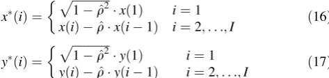
In Step 3, we first assumed a GLM similar to Eq. (3) using the same boxcar functionukðiÞ[29]. Importantly, this differed from Step 1 in terms of the definition of an inde-pendent variablexkðiÞthat was convoluted byukðiÞwith a Gaussian kernel functiong(i) as
xkðiÞ ¼ ðgukÞðiÞ ¼
Xall
n
gðnÞ ukðinÞ
gðiÞ ¼exp ðDiÞ 2
2r2
!
r¼FWHM
2pffiffiffiffiffiffiffiffiffi2ln2:
ð10Þ
The xk computed by Eq. (10) was used after being
nor-malized with its maximum amplitude, and xkðiÞ for all
kwas assigned in a design matrix Xas a column vector.
The gray image ofXis shown in Fig.1b. To examine the
response variable signal y(i), the response vector Y was
composed from time-series rCBF data that were filtered using an HPF with a cutoff frequency of .014 Hz, as
described in Sect.3.2. SummarizingXandYinto a matrix
equation described in Eq. (4), an estimateB^was computed
using the OLS method by
^
B¼XTX1XTY: ð11Þ
Modification 1: Correction of autocorrelation Although
there was no autocorrelation for the error e assumed in
Eq. (3), this assumption was not satisfied by the actual measured data (described as Issue 1 in Introduction) [14]. For this reason, the OLS estimate is an unbiased esti-mator, but it is not the best linear unbiased estimator (BLUE). Hence, the statistical evaluation becomes inac-curate [30] and a type I error (‘‘false’’ brain activation) is more likely to occur. Non-autocorrelation was thus
recovered in Step 3 using the Cochrane–Orcutt
method [48].
First, the following residual errorE2RI was computed
using an estimated parameter B^ obtained by the OLS
method without correction of non-autocorrelation.
E¼YXB^ ð12Þ
Using elements½eð1Þ;eð2Þ;. . .;eðIÞT:¼Ein the vectorE,
the Durbin–Watson ratio (DW) was computed by
DW:¼
PI
i¼2ðeðiÞ ðeði1ÞÞ 2
PI
i¼2ðeðiÞÞ
2 2 ½0;4: ð13Þ
Next, to examine the original e(i), a first-order
autocorre-lation model described by
eðiÞ ¼qeði1Þ þwðiÞ ð14Þ
was assumed using a constantqand a new signalwwith a
mean of zero and no autocorrelation. An alternative valueq^
for qwas specified as
^
q¼1DW=2 ð15Þ
using the value ofDW computed by Eq. (13). Finally, we
performed a new OLS estimate using the following
auto-correlation-corrected x and y from Eqs. (16) and (17).
Then, the newly estimated B^2nd was used in a first-level
analysis of the SPM.
Table 2 Results of statistical test using a convolution matrix method in Step 2: mean values of AIC (at a first-level analysis) andz-values (at a second-level analysis, df=15)
M SD 1 2 3 4 5 6 7 8 9 10 11 12 13 14 15 16 17 18 19 20 21 22 23 24 no filter –5030 2583 3.92 2.03 1.93 5.18 3.51 2.79 2.87 4.83 3.33 3.75 2.88 3.65 1.06 1.85 2.95 2.13 2.65 2.38 3.09 2.37 2.66 2.57 2.82 2.19
0.008 –5304 2533 3.40 2.65 1.52 4.16 4.12 2.41 3.17 5.31 3.21 3.51 2.73 3.89 1.71 1.78 3.44 2.43 2.41 2.53 2.44 3.35 3.30 2.89 3.14 2.35
0.014 –5460 2455 3.14 2.75 1.65 4.21 4.17 2.29 3.32 5.18 3.01 3.52 2.57 3.91 1.78 1.80 3.41 2.59 2.38 2.46 2.11 3.31 3.46 2.89 3.26 2.24
no filter –7041 3012 2.42 1.42 1.38 2.57 3.01 2.35 2.22 4.26 3.49 4.50 1.42 3.71 1.36 0.44 2.82 0.37 –0.04 1.81 2.01 2.75 2.20 1.56 2.20 2.05 0.008 –7369 2558 2.76 1.68 1.20 2.92 3.41 1.84 2.79 4.62 3.89 3.97 2.30 4.09 1.68 1.97 2.80 1.19 0.48 2.22 2.49 3.07 3.13 2.18 2.22 2.35 0.014 –7539 2607 2.65 1.37 1.00 2.53 3.08 1.58 2.53 4.46 3.58 3.72 2.22 3.82 1.51 1.83 2.60 0.97 0.27 1.90 2.15 2.56 3.13 2.13 2.09 2.25
no filter –4479 2896 3.90 2.34 2.08 4.91 3.50 3.46 2.81 4.53 3.54 4.28 2.84 4.07 1.22 1.76 3.81 2.17 2.47 2.20 3.47 2.78 2.77 2.72 2.55 2.86
0.008 –4793 2491 3.46 2.55 1.54 4.75 4.11 2.94 3.23 5.08 3.49 3.90 2.78 4.40 1.99 1.92 3.81 2.75 2.28 2.66 2.92 3.41 3.53 3.13 2.62 2.97
0.014 –4940 2549 3.39 2.41 1.60 4.66 4.05 2.91 3.25 4.91 3.23 3.74 2.51 4.19 2.07 1.98 3.59 2.82 2.29 2.62 2.51 3.17 3.70 3.08 2.71 2.81
Type of CBF
Deoxy
Total Oxy
Channel number AIC
Cufoff freq. [Hz]
xðiÞ ¼
ffiffiffiffiffiffiffiffiffiffiffiffiffi 1q^2
p
xð1Þ i¼1
xðiÞ q^xði1Þ i¼2;. . .;I
ð16Þ
yðiÞ ¼
ffiffiffiffiffiffiffiffiffiffiffiffiffi 1q^2
p
yð1Þ i¼1
yðiÞ q^yði1Þ i¼2;. . .;I
ð17Þ
Modification 2: Consideration of higher-order element
Previous research proposed that the use of the derivative component of an HRF can be effective for NIRS–GLM analysis [31]. This suggestion corresponds well with the current data because an overshoot-like waveform around the rising and falling edges appeared to be approximated by
a derivative term of the canonical HRF, as shown in Fig.3.
Therefore, two new GLM models were considered: (a) a
fourth-order model using a new design matrix X1d 2
RIð4þ1Þ that included the first-derivative terms of x
k described by Eq. (10); and (b) a sixth-order model using
another new design matrixX2d 2RIð6þ1Þthat included the
first- and second-derivative terms. The three models using
X, X1d, and X2d were called HRF-solo (only HRF),
HRF?1.d. (HRF with its first-derivative term), and
HRF?2.d. (HRF with its first- and second-derivative
terms), respectively.
Total accuracy verification and optimal conditionThe results obtained from the first- and second-level analyses
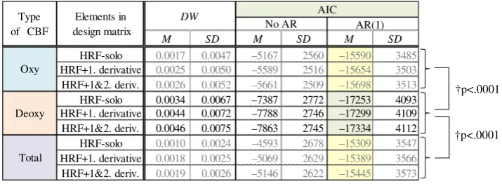
using Modifications 1 and 2 are summarized in Table3.
This table shows the means ofDWand AIC values relevant
to all data channels from all participants. Additional results of the analyses of oxy- and total-Hb data are shown in gray to demonstrate the effects obtained by Modifications 1 and 2. Regarding AIC, the other two cases of ‘‘no correction of
non-autocorrelation (No AR)’’ and ‘‘correction by
Cochrane–Orcutt method (AR(1)), i.e., Modification 1’’ are shown in the same table.
Examination of the values of DW related to
Modifi-cation 1 revealed that they were relatively close to zero in all cases; hence, the assumption of non-autocorrelation
of errors e was not satisfied. This finding supports the
notion that the method used in Step 2 overestimated the statistic, because it did not involve a correction process for non-autocorrelation. The AIC indices also support potential overestimation at Step 2, since the AIC values in AR(1) were two or three times smaller than in No AR. Therefore, the current results demonstrate that
cor-rection for non-autocorrelation is indispensable for
NIRS–SPM analysis, whereas several previous studies
[31,46, 47] have not taken this point into consideration.
In the analysis of Modification 2, Table3 reveals that
the AIC value improved slightly when the GLM con-tained higher-order derivative terms. In summary, we
found that a GLM model using elements of HRF?2.d.
with correction for non-autocorrelation was the most
appropriate for analysis of the rCBF measured during the hand-tracing tasks.
Next the appropriateness of the selection of deoxy-Hb was tested after Modifications 1 and 2 were applied. For the
AIC values under AR(1) conditions shown in Table3,
differences between the deoxy-Hb and oxy-Hb groups, and between the deoxy-Hb and total-Hb groups, were
investi-gated by Welch’st test, respectively. Because each group
included all AIC values computed using HRF-solo,
HRF?1.d., and HRF?2.d. models, the number of samples
in each group was N¼3 models 24 channels16
par-ticipants¼1152. The test revealed that the average of the
AIC values computed using deoxy-Hb was significantly smaller than the average of the values computed using oxy-Hb and total oxy-Hb, as shown on the right side of the
table (the deoxy-Hb vs the oxy-Hb groups: tð1700:4Þ ¼
24:3; p\:0001, the deoxy-Hb vs the total-Hb groups:
tð2299:9Þ ¼ 4:52;p\:0001). Therefore, it can be
con-cluded that deoxy-Hb is better suited for analysis of rCBF since the accuracy of fit to GLM was higher when deoxy-Hb NIRS data were used. Thus, only deoxy-deoxy-Hb data were used in the subsequent analyses.
We repeated the first- and second-level analyses using these modifications with the optimal conditions. The results
are shown in Table 4. The results computed under
condi-tions other than HRF?2.d., i.e., HRF-solo and HRF?1.d.,
are also shown in gray in the table. Contrast matrices were
chosen as C¼ ½ 1 1 1 1 0 ðK¼4Þ and C¼
½ 1 1 1 1 1 1 0ðK¼6Þ for HRF?1.d. and
HRF?2.d., respectively. Table4 demonstrates that
HRF?2.d. and HRF?1.d. were able to detect more
chan-nels showing statistical significance than HRF-solo, and there was a small difference in AIC values. Although the
results in Table 4 show similar tendencies for both
HRF?1.d. and HRF?2.d., we speculate that HRF?2.d.
was more desirable because the AIC value for HRF?2.d.
was smaller than that for the HRF?1.d. model.
Taking the results of Sects.3.1–3.3together, the optimal
guidelines for analyzing NIRS–SPM data for rCBF con-taminated with motion artifacts can be summarized as follows:
• Type of rCBF for SPM analysis: deoxy-Hb.
• Prefilter for rCBF: an HPF with cutoff frequencies of
.014 Hz.
• Method: boxcar-function-based Gaussian convolution
method.
• GLM: a linear model consisting of an HRF computed
using a Gaussian kernel function and its first- and second-derivative terms.
• Modifications: correction for non-autocorrelation by the
Note that these guidelines were obtained by considering a range of issues involved in other NIRS–SPM methods, as
described in Introduction. Issue 1 (the unsatisfied
assumption of normal distribution in measured data) was attenuated by optimization of statistical procedure using AIC and DW indices in Steps 1–3. Issue 2 (the non-auto-correlation problem) was resolved with Modification 1, using the Cochrane–Orcutt method in Step 3. Finally, Issue 3 (related to noise reduction) was resolved in Step 2.
4 Analysis of statistical parametric maps
The spatial distribution of brain activity associated with BS modification was investigated by focusing on the NIRS– SPM results obtained using the optimal conditions derived
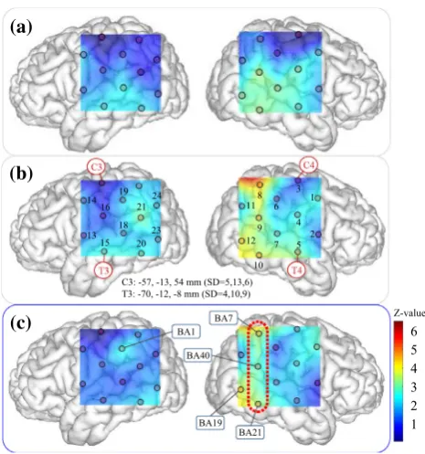
in Sect.3.3. Figure 4 shows z-map images based on the
results shown in Table4. A z-map computed using the
optimal conditions obtained in Step 3 is shown in Fig.4c.
This map is a visualization of the z-values that were
described by blue numbers in Table4. Images (a) and
(b) are otherz-maps based on results obtained in Steps 1
and 2 using the corresponding quasi-optimal conditions.1
The images shown in Fig.4 are montages of a brain
surface image created with the BrainBrowser Surface
Viewer (v2.3.0) [49] and the coloredz-maps. The colored
z-map was drawn by interpolatingz-values with a scattered
data interpolation function (in MATLAB R2015a) after deforming the positions of the NIRS channel grid with reference to C3(4) and T3(4) positions on the MNI
coor-dinate system [50]. Circles and numbers drawn on the z
-map image indicate the position and index of the
measurement channels, respectively. Labels of Brodmann’s area numbers are provided to indicate several channels where strong significant differences were confirmed. First,
Fig.4c shows that the right hemisphere was dominant.
Specifically, significant differences were confirmed in
channels 1, 4, 8–10, and 12 (zð15Þ[2:33;p\:01).
Channel 19, which solely indicates significant differences in the left hemisphere, is close to an area near S1(BA1), which corresponds to the tip of the finger in the cortical homunculus. This finding is in accord with the experi-mental circumstances, since participants used their right hand in Task 2 (while holding a long stick) more strongly than in Task 1 (which only involved one finger). Examin-ing the positions of these significant channels revealed that the following four contiguous areas of the brain were sig-nificantly activated during Task 2: Ar1) somatosensory
association cortex (BA7: z¼3:49;p\:001); Ar2)
supra-marginal gyrus (BA40:z¼2:93;p\:01); Ar3) associative
visual cortex (BA19:z¼3:79;p\:0001); and Ar4) middle
temporal gyrus (BA21: z¼3:46;p\:001). Although a
similar activation pattern at Ar1–Ar4 can be seen in Fig.4b
which was obtained in Step 2, the effects in Step 2 were
likely to be overestimated because thez-values obtained in
Step 2 were larger than that in Step 3, despite the larger AIC values in Step 3. Therefore, it seems reasonable to
conclude that the pattern in thez-map image (c) obtained
by Step 3 is a feature of the BS modification related to the hand-tracing task.
Areas BA7 and BA40 related to Ar1 and Ar2 are part of the parietal association cortex. It has been found that damage to these areas causes spatial perception impair-ment [51]. The parietal association cortex forms the pari-etal lobe in combination with the S1 area, and the right
parietal lobe has been closely linked to spatial
skills [52,53]. Specifically, a bimodal neuron responding
to both visual and somatic senses has been reported to exist in the intraparietal sulcus (which is located near BA7) in
Table 3 Durbin–Watson ratios and AICs when a boxcar-function-based Gaussian convolution method was applied at Step 3. (Color table online)
†p<.0001
†p<.0001
M SD M SD M SD
0.0017 0.0047 –5167 2560 –15590 3485 0.0025 0.0050 –5589 2516 –15654 3503 0.0026 0.0052 –5661 2509 –15698 3513 0.0034 0.0067 –7387 2772 –17253 4093 0.0044 0.0072 –7788 2746 –17299 4109 0.0046 0.0075 –7863 2745 –17334 4112 0.0010 0.0024 –4593 2678 –15309 3547 0.0018 0.0025 –5069 2629 –15389 3566 0.0019 0.0026 –5146 2622 –15445 3573 Deoxy
HRF-solo HRF+1. derivative
HRF+1&2. deriv.
AIC
No AR AR(1)
Total
HRF-solo HRF+1. derivative
HRF+1&2. deriv. Oxy
HRF-solo HRF+1. derivative
HRF+1&2. deriv. Elements in design matrix Type
of CBF
DW
1 The quasi-optimal condition at Step 1 was ‘‘rCBF type: deoxy, time
the right parietal lobe [54]. In addition, the intraparietal sulcus was reported to be associated with the BS in a study of the RHI [55]. These previous findings regarding the right-hemisphere dominance of the parietal lobe are
con-sistent with the current SPM results shown in Fig.4c.
Taken together, these results suggest that the brain areas involved in spatial perception may have been activated when BS extension was required during the use of a long stick in the current study. In addition, the inferior parietal
lobule consists of BA40 and the angular gyrus (BA39),2
and the right inferior parietal cortex is related to own-body
perception and the illusion of motion [56, 57].
Interest-ingly, it has been reported that out-of-body
experi-ences [58,59] and phantom sensations [60] can be induced
by stimulating the angular gyrus, one of the areas associ-ated with the BS.
BA19 (in Ar3) is involved in the recognition of the shape and color of objects [61]. In the present study, we speculate that this area may have become active when participants visually examined the characters traced by their fingers. This characteristic may be a feature of the BS extension because the BS is visually dominant [62]. Acti-vation in this area, however, does not necessarily indicate general BS extension because the cognitive processing involved in recognizing Hiragana characters might have also caused neural responses in this region. Moreover, BA21 (in Ar4) is reported to be activated when subjects are engaged in contemplating distance [63]. In the current study, this brain area may have been activated during the estimation of the distance from their own body to the tip of the stick, which would be required to extend the BS spatially.
Taken together, this evidence suggests that the brain activation we observed in contiguous areas in BA7–BA40– BA21 may be related to BS extension during a hand-trac-ing task.
5 Conclusions and future research
This study described an optimized statistical analysis pro-cedure for NIRS–SPM analysis that involves dealing with rCBF data contaminated by motion artifacts. In addition, we identified the spatial distribution of brain activity associated with BS modification using a hand-tracing task that involved an extension of the BS. Three methodological options were evaluated in turn to determine the optimal conditions for NIRS–SPM analysis: a model-free method in Step 1, a convolution matrix method in Step 2, and a boxcar-function-based Gaussian convolution method in Step 3.
In Step 1, it was found that the actual rCBF waveform during this task could be approximated by a rounded trapezoidal waveform similar to the convolved response of a boxcar with a Gaussian function. Moreover, deoxy-Hb was found to be appropriate for the NIRS–GLM in this
Table 4 Results of statistical test using a boxcar-function-based Gaussian convolution method in Step 3:z-values in a second-level analysis for three kinds of design matrices,df¼15
AIC:AR(1) 1 2 3 4 5 6 7 8 9 10 11 12 13 14 15 16 17 18 19 20 21 22 23 24 M –1.81 – 0.96 – 0.95 –1.20 0.91 – 0.62 1.29 2.42 0.33 0.36 0.95 0.28 0.10 0.21 – 0.15 – 0.32 – 0.31 – 0.61 1.28 –0.29 0.18 0.84 0.46 1.04 –17253 – 0.14 2.43 1.58 2.09 2.20 0.73 2.39 3.00 2.92 2.88 1.79 3.24 1.37 1.55 1.72 1.25 –1.08 1.21 3.60 2.08 0.53 1.94 0.96 –0.06 –17299
2.74 0.90 2.13 2.37 1.79 1.15 1.99 3.49 2.93 3.46 1.81 3.79 1.43 1.31 1.46 1.43 – 0.19 1.07 2.65 2.26 1.49 1.83 2.00 1.28 –17334
Elements in design matrix
HRF-solo HRF +1. derivative
HRF +1&2. deriv.
Channel number
Blue cells showz[2:33ðp\:01Þ, and red cells showz[3:09ðp\:001Þ. (Color table online)
(a)
(b)
(c)
BA7BA40
BA19 BA21 BA1
1
2 3
4 6
7 8
9 11
12 14
13 15 16
18 19
20 21
23 24
6 5 4 3 2 1 Z-value 5
10 C3: -57, -13, 54 mm (SD=5,13,6) T3: -70, -12, -8 mm (SD=4,10,9)
Fig. 4 Statistical parametric maps (z-map images,df¼15):a model-free method (Step 1); b convolution matrix method (Step 2); c a boxcar-function-based Gaussian convolution method (Step 3). (Color figure online)
2 The BA39 area was out of the measurable range of this NIRS
experiment, as indicated by the results of diagnostic screening indices concerning individual variance and AIC, which was confirmed in Step 3. In Step 2, to enhance statistical accuracy, conditions for eliminating low-fre-quency noise and modifying the DoF for statistical testing were investigated using the AIC. In Step 3, correction of non-autocorrelation with derivative components of HRF was applied to a GLM for SPM, by calculating the DW ratio and AIC values. Finally, credible SPM guidelines for NIRS data were obtained. Examination of the best SPM results confirmed that contiguous areas in BA7–BA40– BA21 (BA7: somatosensory association cortex; BA40: supramarginal gyrus; BA21: middle temporal gyrus) in the
right hemisphere became significantly active (p\:001,
p\:01, andp\:001, respectively) during the hand-tracing
tasks, potentially representing BS modification.
Future research could incorporate the NIRS–SPM method described here to exogenously enhance the ability of BS extension using electrical stimuli.
Acknowledgements The experiments were performed by Akira Ichinose, Takumi Matsumura, Noriko Kimura, Kei Kawahara, and Toshifumi Chikaraishi. This research would not be possible without the many participants who kindly took part in this study. This research was in part supported by a JSPS Grant-in-Aid for Exploratory Research (Grant No. 25630179) and Grant-in-Aid for Scientific Research (C) (Grant No. 15K06153), Japan.
Compliance with ethical standards
Conflict of interest The author declares that they have no conflict of interest.
Open Access This article is distributed under the terms of the Creative Commons Attribution 4.0 International License (http://crea tivecommons.org/licenses/by/4.0/), which permits unrestricted use, distribution, and reproduction in any medium, provided you give appropriate credit to the original author(s) and the source, provide a link to the Creative Commons license, and indicate if changes were made.
References
1. Rizzolatti G, Fadiga L, Fogassi L, Gallese V (1997) The space around us. Science 277(5323):190–191
2. Blakeslee S, Blakeslee M (2007) The body has a mind of its own. Random House, New York
3. Maravita A, Iriki A (2004) Tools for the body (schema). Trends Cogn Sci 8(2):79–86
4. Galfano G, Pavani F (2005) Long-lasting capture of tactile attention by body shadows. Exp Brain Res 166(3–4):518–527 5. Won AS, Bailenson J, Lee J, Lanier J (2015) Homuncular
flex-ibility in virtual reality. J Comput Med Commun 20(3):241–259 6. Head H, Holmes G (1911) Sensory disturbances from cerebral
lesions. Brain 34(2–3):102–254
7. Iriki A, Tanaka M, Iwamura Y et al (1996) Coding of modified body schema during tool use by macaque postcentral neurons. J Neurosci 7:2325–2330
8. Athanasiou A, Lithari C, Kalogianni K, Klados MA, Bamidis PD (2012) Source detection and functional connectivity of the sen-sorimotor cortex during actual and imaginary limb movement: a preliminary study on the implementation of e-connectome in motor imagery protocols. Adv Hum Comput Interact. doi:10. 1155/2012/127627
9. Iacobonil M, Woods RP, Brass M, Bekkering H, Mazziotta JC, Rizzolatti G (1999) Cortical mechanisms of human imitation. Science 286(5449):2526–2528
10. Fadiga L, Fogassi L, Pavesi G, Rizzolatti G (1995) Motor facil-itation during action observation: a magnetic stimulation study. J Neurophysiol 73(6):2608–2611
11. Rizzolatti G, Craighero L (2004) The mirror-neuron system. Ann Rev Neurosci 27:169–192
12. Botvinick M, Cohen J (1998) Rubber hands ‘feel’ touch that eyes see. Nature 391:756–756
13. Armel KC, Ramachandran VS (2003) Projecting sensations to external objects: evidence from skin conductance response. R Soc B: Biol Sci 270(1523):1499–1506
14. Shimada S, Hiraki K, Oda I (2005) The parietal role in the sense of self-ownership with temporal discrepancy between visual and proprioceptive feedbacks. Neuroimage 24:1225–1232
15. Shimazu T, Suzuki S (2014) A preliminary study of functional brain activity concerning modification of a body schema on hand manipulation. In: NCSP. RISP, pp 553–554
16. Goodwin GM, McCloskey DI, Matthews PB (1972) The contri-bution of muscle afferents to kinaesthesia shown by vibration induced illusions of movement and by the effects of paralysing joint afferents. Brain 95(4):705–748
17. Naito E, Ehrsson HH, Geyer S, Zilles K, Roland PE (1999) Illusory arm movements activate cortical motor areas: a PET study. J Neurosci 19:6134–6144
18. Lackner JR (1988) Some proprioceptive influences on the per-ceptual representation of body shape and orientation. Brain 111:281–297
19. Ehrsson HH, Kito T, Sadato N, Passingham RE, Naito E (2005) Neural substrate of body size: illusory feeling of shrinking of the waist. PLoS Biol 3(12):2200–2207
20. Gandevia SC (1985) Illusory movements produced by electrical stimulation of low-threshold muscle afferents from the hand. Brain J Neurol 108:965–981
21. Hoffmann M, Marques HG, Arieta AH, Sumioka H, Lungarella M, Pfeifer R (2010) Body schema in robotics: a review. IEEE Trans Auton Ment Dev 2(4):304–324
22. Oyebode F (1998) Sims’ symptoms in the mind: an introduction to descriptive psychopathology. Saunders Elsevier, Edinburgh 23. Gross CG, Graziano MSA (1995) Multiple representations of
space in the brain. Neuroscientist 1(1):43–50
24. Lathan CE, Tracey M (2002) The effects of operator spatial perception and sensory feedback on human–robot teleoperation performance. J Presence 11(4):368–377
25. Steptoe W, Steed A, Slater M (2013) Ownership and control of extended humanoid avatars. IEEE Trans Vis Comput Graph 19(4):583–590
26. Nakamura S, Mochizuki N, Konno T, Yoda J, Hashimoto H (2015) Research on updating of body schema using AR limb and measurement of the updated value. IEEE Syst J. doi:10.1109/ JSYST.2014.2373394
27. Vignemont F (2010) Body schema and body image-pros and cons. Neuropsychologia 48(3):669–680
28. Friston KJ, Ashburner JT, Kiebel SJ, Nichols TE, Penny WD (2007) Statistical parametric mapping: the analysis of functional brain images. Academic, Amsterdam
(2004) Towards a standard analysis for functional near-infrared imaging. Neuroimage 21(1):283–290
30. Plichta MM, Heinzel S, Ehlis A-C, Pauli P, Fallgattera AJ (2007) Model-based analysis of rapid event-related functional near-in-frared spectroscopy (NIRS) data: parametric validation study. Neuroimage 35:625–634
31. Uga M, Dan I, Sano T, Dan H, Watanabe E (2014) Optimizing the general linear model for functional near-infrared spec-troscopy: an adaptive hemodynamic response function approach. Neurophotonics 1(1):1–10
32. Mardia KV, Kent JT, Bibby JM (1979) Multivariate analysis. Academic, San Diego
33. SPM software (2015) SPM web. http://www.fil.ion.ucl.ac.uk/ spm/. Accessed 7 August 2016
34. Miall RC, Wolpert DM (1996) Forward models for physiological motor control. Neural Netw 9(8):1265–1279
35. Sober SJ, Sabes PN (2003) Multisensory integration during motor planning. J Neurosci 23(18):6982–6992
36. Suzuki S, Kobayashi H (2008) Brain monitoring analysis of voluntary motion skills. J Assist Robot Mech 9(2):20–30 37. Suzuki S, Harashima F, Furuta K (2010) Human control law and
brain activity of voluntary motion by utilizing a balancing task with an inverted pendulum. Adv Hum Comput Interact. doi:10. 1155/2010/215825
38. Holmes AP, Friston KJ (1998) Generalisability, random effects and population inference. Neuroimage 7:754
39. Hoshi Y, Onoe H, Watanabe Y, Andersson J, Bergstrom M, Lilja A, La˚ngstro¨m B, Tamura M (1994) Non-synchronous behavior of neuronal activity, oxidative metabolism and blood supply during mental tasks in man. Neurosci Lett 19(172):129–133
40. Hoshi Y, Kobayashi N, Tamura M (2001) Interpretation of near-infrared spectroscopy signals: a study with a newly developed perfused rat brain model. J Appl Physiol 90:1657–1662 41. Strangman G, Culver JP, Thompson JH, Boas DA (2002) A
quantitative comparison of simultaneous BOLD fMRI and NIRS recordings during functional brain activation. Neuroimage 17(2):719–731
42. Obrig H, Wenzel R, Kohl M, Horst S, Wobst P, Steinbrink J, Thomas F, Villringer A (2000) Near-infrared spectroscopy: does it function in functional activation studies of the adult brain? J Psychophysiol 35(2–3):125–142
43. Schroeter ML, Zysset S, Kupka T, Kruggel F, von Cramon DY (2002) Near-infrared spectroscopy can detect brain activity dur-ing a color-word matchdur-ing stroop task in an event-related design. Hum Brain Mapp 17(1):61–71
44. Friston KJ, Holmes AP, Poline J-B, Grasby PJ, Williams SCR, Frackowiak RSJ, Turner R (1995) Analysis of fMRI time-series revisited. Neuroimage 2(1):45–53
45. Fearsa TR, Benichoua J, Gaila MH (1996) A reminder of the fallibility of the Wald statistic. Am Stat 50(3):226–227 46. Friston KJ, Holmes AP, Worsley KJ, Poline J-P, Frith CD,
Frackowiak RSJ (1995) Statistical parametric maps in functional
imaging: a general linear approach. Hum Brain Mapp
2(4):189–210
47. Worsley KJ, Friston KJ (1995) Analysis of fMRI time-series revisited again. Neuroimage 2(3):173–181
48. Cochrane D, Orcutt GH (1949) Application of least squares regression to relationships containing auto-correlated error terms. J Am Stat Assoc 44(245):32–61
49. Official Site of BrainBrowser Surface Viewer. https://brain browser.cbrain.mcgill.ca/. Accessed 7 August 2016
50. Vitali P, Avanzini G, Caposio L, Fallica E, Grigoletti L, Mac-cagnano E, Rigoldi B, Rodriguez G, Villani F (2002) Cortical location of 10–20 system electrodes on normalized cortical MRI surfaces. J Bioelectromagnetism 4(2):147–148
51. Goodale MA, Meenan JP, Bulthoff HH, Nicolle DA, Murphy KJ, Racicot CI (1994) Separate neural pathways for the visual anal-ysis of object shape in perception and prehension. Curr Biol 4(7):604–610
52. Vallar G, Perani D (1986) The anatomy of unilateral neglect after right-hemisphere stroke lesions. a clinical/CT-scan correlation study in man. Neuropsychologia 24(5):609–622
53. Hillis AE, Newhart M, Heidler J, Barker PB, Herskovits EH, Degaonkar M (2005) Anatomy of spatial attention: insights from perfusion imaging and hemispatial neglect in acute stroke. J Neurosci 25(12):3161–3167
54. Naito E, Ehrsson HH (2001) Kinesthetic illusion of wrist
movement activates mortor-related areas. Neuroreport
12:3805–3809
55. Ehrsson HH, Spence C, Passingham RE et al (2004) That’s my hand! activity in premotor cortex reflects feeling of ownership of a limb. Science 305(5685):875–877
56. Berlucchi G, Aglioti S (1997) The body in the brain: neural bases of corporeal awareness. Trends Neurosci 20:560–564
57. Damasio AR (1999) The feeling of what happens: body and emotion in the making of consciousness. Harcourt Brace, New York
58. Blanke O, Landis T, Spinelli L, Seeck M (2004) Out-of-body
experience and autoscopy of neurological origin. Brain
127:243–258
59. Ehrsson HH (2007) The experimental induction of out-of-body experiences. Science 317:1048–1048
60. Arzy S, Seeck M, Ortigue S, Spinelli L, Blanke O (2006) Induction of an illusory shadow person: stimulation of a site on the brain’s left hemisphere prompts the creepy feeling that somebody is close by. Nature 443(21):287
61. Kaas JH (1996) Theories of visual cortex organization in pri-mates: areas of the third level. Prog Brain Res 112:213–221 62. Beers RJ, Sittig AC, Denier GJJ (1996) How humans combine
simultaneous proprioceptive and visual position information. Exp Brain Res 111(2):253–261
63. Acheson DJ, Hagoort P (2013) Stimulating the brain’s language network: syntactic ambiguity resolution after TMS to the inferior frontal gyrus and middle temporal gyrus. J Cogn Neurosci 25(10):1664–1677