The effect of transmission variance on observer placement for source-localization

R E S E A R C H

Open Access

The effect of transmission variance on

observer placement for source-localization

Brunella Spinelli

, L. Elisa Celis and Patrick Thiran

*Correspondence: [email protected] École Polytechnique Fédérale de Lausanne (EPFL), Lausanne, Switzerland

Abstract

Detecting where an epidemic started, i.e., which node in a network was the source, is of crucial importance in many contexts. However, finding the source of an epidemic can be challenging, especially because the information available is often sparse and noisy. We consider a setting in which we want to localize the source based exclusively on the information provided by a small number ofobservers– i.e., nodes that can reveal if and when they are infected – and we study where such observers should be placed. We show that the optimal observer placement depends not only on the topology of the network, but also on the variance of the node-to-node transmission delays. We consider both low-variance and high-variance regimes for the transmission delays and propose algorithms for observer placement in both cases. In the low-variance regime, it suffices to only consider the network-topology and to choose observers that, based on their distances to all other nodes in the network, can distinguish among possible sources. However, the high-variance regime requires a new approach in order to guarantee that the observed infection times are sufficiently informative about the location of the source and do not get masked by the noise in the transmission delays; this is

accomplished by additionally ensuring that the observers are not placed too far apart. We validate our approaches with simulations on three real-world networks. Compared to state-of-the-art strategies for observer placement, our methods have a better performance in terms of source-localization accuracy for both the low- and the high-variance regimes.

Keywords: Source localization, Epidemics, Sensor placement

Introduction

Regardless of whether a network comprises computers, individuals or cities, in many applications we want to detect whenever any anomalous or malicious activity spreads across the network and, in particular, where the activity originated. In effect, we wish to answer questions such aswhat was the origin of a worm in a computer network?,who was the instigator of a false rumor in a social network?andcan we identify patient zero of a virulent disease? We call the spread of any such phenomenon anepidemicand its orig-inator thesource. Clearly, monitoring all network nodes is not feasible due to cost and overhead constraints: The number of nodes in the network may be prohibitively large and some of them may be unable or unwilling to provide information about their state. Thus, studies have focused on how to localize the source based on information from a few nodes (calledobservers). Given a set of observers, many models and estimators for

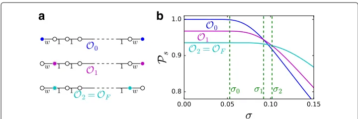
source localization have been developed (Pinto et al. 2012; Louni and Subbalakshmi 2014; Zhang et al. 2016). However, theselectionof observers has not yet received a satisfactory answer: Most methods consider only the structure of the network when placing observers. However, depending on the particular epidemic model, the expected transmission delay between two nodes, and its variance, can differ widely and this can have a significant impact on source localization. We show that different transmission models require differ-ent observer placemdiffer-ents as illustrated in Figs. 1 and 2: As the variance of the transmission delays changes, the optimal set of observers also changes.

The difficulties faced in finding the optimal observers for source localization are two-fold. First, computing the likelihood of a node being the source conditional on the available observations can be computationally prohibitive (Shah and Zaman 2011; Pinto et al. 2012); evaluating the probability of correct localization given a set of observers is, in general, even harder. Second, the optimal selection of a limited number of observers is NP-hard, even when the transmission delays are deterministic. We take a principled approach that begins with considering deterministic transmission delays (zero-variance

regime), and we build on this intuition in order to develop heuristics for bothlow-variance

andhigh-varianceregimes for the transmission delays.1

Model and problem statement

Transmission model.We assume that the epidemic spreads in a known contact network. Thetransmission delaythrough edgeuv, i.e., the time it takes for a nodeuto infect a neighbor nodevis encoded by the random variableXuv.

We assume a transmission model which is both natural and versatile as it comprises deterministic transmissions, which we callzero-variance, and arbitraryrandom indepen-dent transmission models. We study, in particular, how theamountof randomness (i.e., the variance ofXuv) in the transmission delays affects the choice of observers for source localization. Towards this, we are the first to separately analyze two different regimes for the amount of randomness of the transmission delays:low-varianceandhigh-variance. A dichotomy exists between the two, and our approach for observer placement differs.

Fig. 1Sequence of optimal observer placements for increasing transmission variance. We assume the transmission transmission delays{Xuv}uv∈Eto be such thatE[Xuv]=wuv∈R+and such that the variance is a growing function of a variance parameterσ, i.e., Var(Xuv)=g(wuv,σ )withg(x, 0)=0 for allx∈R+. For

σ ∈(0,σ0)the transmission delays are effectively deterministic (i.e.,σdoes not affect source localization). For

σ ∈(σ0,σ1),σaffects the accuracy of source localization but the optimal observer placement is stillO0. For

largerσ, the optimal observer placement might change, possibly multiple times (Okdenotes the optimal

a

b

Fig. 2Optimal observers for Gaussian-distributed transmission delays with unit mean and standard deviationσon a path graph. In this casePsand, consequently, the optimal observer placements, can be

explicitly computed.adifferent observer placements;btheir performance in terms of probability of success Psforw=20 and 30 edges

We use the SI epidemic model adopted, e.g., in (Pinto et al. 2012; Luo and Tay 2012). Nonetheless, since our methods for source localization only uses the time at which the sensors are first infected (no assumption on recovery or re-infection dynamics is made), they can be applied to any epidemic model, including the well known SIS or SIR (provided that nodes do not recover before infecting their neighbors).

Source localization.We assume that there is asinglesource that initiates the epidemic, an extension of our results to the case the case of multiple sources could use the recent work by Zhang et al. (2015) on a related problem and is left for future work.

LetO⊆Vbe the set of observer nodes (which we will select). We assume we know the time at which each observer is infected, and we refer to this vector of infection times as

T_O. KnowingT_O is a standard and realistic assumption (Netrapalli and Sanghavi 2012). We want to identify the source using only the information contained inT_O.

We use maximum likelihood estimation (MLE) to produce an estimateˆs of the true

unknown sourcesas in (Pinto et al. 2012). This approach is common (see e.g., (Shah and Zaman 2011; Dong et al. 2013)), although the exact form of the estimator depends on the model and assumptions. In our case we have

ˆ

s∈argmax_s∈VP(TO|s=s)π(s),

whereπ denotes the prior on the position of the source. In this paper, unless otherwise specified we assumeπto be uniform (i.e.,π(s)=1/nfor all nodess∈Vwheren= |V|). Metrics.We assume that we are given abudget kon the number of observers we can use, and that we must select our observersonce and for all, i.e., independently of any particular epidemic instance. In order to select thebest set of observersOof size kwe must first define our metric of interest. In this work we are mainly interested in thesuccess probability

Ps=P(ˆs=s)

the real source (Celis et al. 2015; Louni et al. 2015), i.e.,E[d(s,ˆs)], whereddenotes the distance between two nodes in the network.

In “Metrics for source localization” section we present several alternatives to these two metrics, including worst-case metrics, and show that optimizing different metrics can require different sets of observers.

Main contributions

Low-variance regime.When the variance in the transmission delays is low(see “The low-variance regime” section), we prove that the set of optimal observers is exactly the optimal set for the zero-variance regime. In the zero- and low- variance regime, both the probability of successPs(as well as other possible metrics of interest) can be explicitly computed. Despite this seeming simplicity, the problem remains NP-hard. We tackle the problem by using its connection with the well-studied related Double Resolving Set (DRS) problem (Cáceres et al. 2007) that minimizes the number of observers for correct local-ization. This minimum number is, in many cases, still prohibitively large, and can be as much asn−1, hence we cannot use this approach directly. However, from the connec-tion between observer placement and DRS, we find inspiraconnec-tion for our algorithm which, by selecting one observer at a time until the budget is exhausted in order to reach a DRS set, greedily improvesPs.

High-variance regime.When the noise in the transmission delays ishigh, it is no longer negligible and it poses an additional challenge to source localization; in effect, the accu-mulation of noise from node to node as the epidemic spreads might no longer enable us to distinguish between two potential sources, especially when they are bothfarfrom all observers. Hence, we muststrengthenthe requirements for observer placement in order to ensure that the nodes can be distinguished by observers that arenearto them; this nearness is a function of the noise, of the budgetk, and of the network topology. We define a novel objective function that both maximizes the success probability and imposes auniformspread of observers in the network. Taking inspiration from the low-variance regime, we design an algorithm that greedily maximizes this new objective (see “The high-variance regime” section).

Preliminaries Model

LetG =(V,E,w)be a weighted network. For ease of presentation we assume the graph is undirected andwuv = wvu; however our definitions and approach extend straight-forwardly to the directed case. Assumingu is infected, the weightwuv ∈ R+ of edge

uv∈Erepresents the expected time it takes foruto infectv. The edge weights induce a

weighted-distancemetricdonG:d(u,v)is the length of the shortest path fromutov. We also sometimes consider the minimum number of edges on a path connecting two nodes, which we call thehops-distance.

We assume that the epidemic is initiated by a single unknown sourcesat an unknown timet. The fact that thetime tat which an epidemic starts is unknown adds a significant difficulty to the problem because asingleobservation is notper seinformative. Instead, in order to localize the source, we must use thedifferencesbetween the observed infection times.

If a nodeugets infected at timetu, a non-infected neighborvofuwill become infected at timetv= tu+XuvwhereXuvis a random variable. A large part of the epidemic liter-ature models transmission delays with exponential random variables. However we make a different modeling choice for two reasons. First, we are interested in decoupling the transmission variance and the average transmission time (for exponential random vari-ables, mean and variance cannot be tuned independently). Second, in many applications it has been suggested that the transmission delays can be less-skewed than exponential random variables (Cha et al. 2009; Lessler et al. 2009; Vergu et al. 2010). For every edgeuv

we assumeXuvto be a symmetric and non-negative2random variable. We do not make

any strong assumption on the distribution of the transmission delaysXuv: we only assume that their mean is equal to the edge weights, i.e.,E[Xuv]=wuvfor everyuv∈E, and that their variance is an increasing function of both the edge weight and of a variance parame-terσ, that is, Var(Xuv)=g(wuv,σ), wheregdepends on the particular distribution ofXuv andg(x, 0)=0 for allx∈R+.

If the variance is zero, or if it is low compared to edge weights, network distances are a good proxy for time delays (see “Identification of the source class” section). We refer to this setting as alow-varianceregime, as opposed to thehigh-varianceregime in which time delays are very noisy and network distances no longer work as a proxy for time delays.

Distance vectors and node equivalence

We start with a few definitions. Our setting is similar to that of Celis et al. (2015).

Definition 1(Equivalence)LetG = (V,E)andO ⊆ V with|O| = k ≥ 2be a set of observers onG. A node u is said to be equivalent to a node v (which we write u∼v) if and only if, for every oi,oj∈O

d(u,oi)−d(u,oj)=d(v,oi)−d(v,oj). (1)

Fig. 3An unweighted network with two observer nodeso1ando2.Different shapesrepresent different

equivalence classes, i.e., groups of nodes which are not distinguishable from the point of view of the observers. In this example there areq=5 equivalence classes

When the variance is zero, given an observer set, we candistinguish ufromvif there exist two observersoi,ojsuch that Eq. (1) doesnothold foru,vandoi,oj, i.e.,

d(u,oi)−d(u,oj)=d(v,oi)−d(v,oj),

which means that [u]_O=[v]_O.

The problem of finding the minimum-size set of nodesS, such that for everyu,vin a network there existsi,sj∈Sfor whichd(u,si)−d(u,sj)=d(v,si)−d(v,sj)is known as theDouble Resolving Set(DRS)Problem(Cáceres et al. 2007), while the minimum size of

a DRS is known as theDouble Metric Dimension(DMD) of the network. Our problem

differs from DRS because we focus on the more realistic context in which, due to limited resources, we want to allocate afinite budgetin order to optimize source localization3 (as opposed to minimizing the number of observers for perfect localization, which is, in many cases, still prohibitively large). However, the connection between our problem and DRS paves the way for a principled approach to observer placement.

We now define, for everyv∈ V, adistance vector, which, as we will see in Lemma 1, mathematically captures equivalence in a manner that is easy to work with.

Definition 2(Distance Vector)LetG =(V,E),O⊆V with|O| =k≥2and o1∈O. For each node v∈V the distance vector of v with respect to o1isds,o1 ∈Rk−1with entries d(v,oi+1)−d(v,o1)for1≤i≤k−1.

The following lemma, similar in spirit to Lemma 3.1 in (Chen et al. 2014), shows that the equality between distance vectors of different nodes does not depend on the choice of thereference observer o1.

Lemma 1Let G = (V,E)andO ⊆ V with|O| = k ≥ 2and let u,v ∈ V . Then,

[u]_O=[v]_Oif and only ifdu,o1 =dv,o1, independently of the choice of the reference observer o1.

Metrics for source localization

In this section we define some possible metrics of interest for the source-localization problem and we show that optimizing these metrics can effectively require different sets of observers.

For ease of exposition, we restrict ourselves to the zero-variance regime and we assume that the prior distribution on the position of the source is uniform.

only correctly identify theclassto whichsbelongs and we produce an estimated source ˆ

s∈[s] sampling from [s] uniformly.

We adopt two metrics to evaluate the performance of our algorithms: the success

probabilityPsand theexpected error distanceD.

The success probabilityPs is defined asP(ˆs = s). In the low-variance case it can be easily computed. Letqbe the number of equivalence classes identified by an observer set O, then

Ps = [u]⊆V

P(ˆs=s|s∈[u])P(s∈[u])

=

[u]⊆V

1

|[u]| ·|[un]| = 1n

[u]⊆V

1= q_n. (2)

Note thatPs=1 if and only if all equivalence classes are singletons.

The expected error distanceDdef= E[d(ˆs,s)] can also be computed, in the low-variance case, from the partition in equivalence classes:

D =E[d(s,ˆs)]

=

s∈V

P(s =s)

u∈[s]

P(ˆs=u|s=s)d(s,u)

= 1

n

s∈V

1

|[s]|

u∈[s] d(s,u),

(3)

where again D = 0 if and only if all equivalence classes are singletons. An

analo-gous expression for the hops-distance (instead of the weighted distance as in (3)) is also considered in the experimental evaluation in “Empirical results” section.

MaximizingPs (respectively, minimizing E[d(s,ˆs)]) we minimize the probability of ˆ

s=s(respectively, the average distance betweensandˆs). Other natural metrics of inter-est are theworst-caseversions of these metrics over the vertex setV, i.e., theminimum probability of successPs def= min[s]⊆VPs|s∈[s]and themaximum distance betweenˆs and s, denoted byD.Pscan be computed as

Ps= min

[u]⊆V 1 |[u]|,

andDas

D=max

[s]⊆Vtmax,v∈[s]d(t,s).

These last two metrics are relevant, for example, in an adversarial setting (e.g., in the case of bio-warfare), where if the observers are known, the adversary would select theworst

location for the source.

A last natural metric, which is intermediate between average and worst-case metrics, is theexpected maximum distancebetween the true and the estimated source that we define asDdef= Es[ max(d(s,ˆs))]. We have

D=Es[ maxd(s,ˆs)]=

s∈V 1

n

max t∈[s]d(s,t)

.

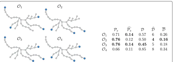
Fig. 4A tree with different sets ofk=4 observers (blue). The table displays the values of different metrics for the observer sets. The best values for each metric are inbold type. The remaining possible choices ofk=4 observers within the leaves set are omitted either because they are equivalent to one of the placements considered or because they do not optimize any of the metrics examined

observers represented in the four sub-figures. With an argument similar to that of Celis et al. (2015), it can be shown that, for all metrics considered and for any budgetksmaller than the number of leaves, the optimal observer set is a subset of the leaves set.4_Hence

we only consider observer sets contained in the leaves set. Figure 4 shows the values ofPs,

Ps,D,DandDfor a subset of the possible observer placements contained in the leaves set and having cardinalityk=4. These placements include those that optimizePs,Ps,D,

DandD.

The low-variance regime Identification of the source class

We formalize how we can localize the source in the zero-variance setting, i.e., whenXuv=

wuvfor every edge(u,v).

For every observer oi ∈ O, denote by ti the time at which oi gets infected. In the zero-variance setting, the observed infection times of nodeso2,. . .,oK with respect to observero1, i.e., the vectorτ def= t2−t1,. . .,tk −t1, is exactly the distance vector of the unknownsourceswith respect too1. Then, if for everyu,v∈V[u]O=[v]O, the source

can be always correctly identified by finding the node whose distance vector matches the observed infection times. Theorem 1 proves that this is true also in a more general

low-varianceframework where we are always able to identify the equivalence class to which the real source belongs by looking at the distances between the distance vectors {dv,o1,v∈V}and the vectors of infection timesτ.

Theorem 1LetG=(V,E)be a network of size n,O⊆V and fix o1∈O. Call

δ min

u,v:du,o₁=dv,o₁du,o1−dv,o1∞

and call D the maximum distance in hops in any shortest path between any node and any observer.

If the transmission delays are such that for each uv∈E, Xuv∈[wuv(1−ε),wuv(1+ε)]

withε < ε0 ₄δ_D then for every v ∈[s]dv,o1 −τ∞ ≤ 2εD and for every v ∈/ [s]

ProofLettobe the infection time ofo∈O. When the source isswe have

to−t≤d(s,o)(1+ε). (4)

Moreover, ifQis the collection of all paths connectingsandoand, forp∈Q, ifdp(s,o)

is the (weighted) length of pathpwe have

to−t≥min p∈Qdp(s

_{,o)(1−ε)=d(s,o)(1−ε). (5)}

Combining inequalities (4) and (5) forobeing, respectively,oando1and callingt1(resp., to) the infection time of the reference observero1(resp.,o), we have

|to−t1−d(s,o)+d(s,o1)| ≤

ε(d(s,o)+d(s,o1))≤2εD.

Since for everyv∈[s]dv,o1 =ds,o1, we conclude that for everyv∈[s],dv,o1−τ∞≤

2εD.

Take nowv ∈/[s] and assume by contradiction that dv,o1 − τ ≤ 2εD. Using the

triangular inequality and the hypothesisε < δ/4Dwe have

ds,o1−dv,o1∞ ≤ ds,o1−τ∞+ dv,o1−τ∞

≤4εD< δ,

which contradicts the definition ofδ. Hence for everyv∈/[s],dv,o1−τ∞>2εD.

Note that hereε0plays the role ofσ0in Fig. 1 in the sense that it is an upper-bound

on a regime in which the delays are effectively deterministic and the variance of the transmission delays does not affect the accuracy of source localization.

If additional conditions on the weights or on the network topology are made, more refined versions of Theorem 1 can be proven. For example, in atreewith integer weights, due to the uniqueness of the path between two any vertices, it can be shown thatδ ≥ 2 and Theorem 1 holds forε < ε0 ₂1_D.

For the remainder of this section, we will assumeε < δ/4D, which we call the low-variance regime.

Estimation of the source

Assume that a prior probability distribution on the identity of the source is given, i.e., that we knowπ(v) def= P(s = v). After the source class [s]_O is identified based onτ as described in “Identification of the source class” section, we let our estimated sourceˆs

be chosen at random from the conditional probabilityπ|[s](u) def= P(s = v|v∈[s]). If

a priorπis not known, we select the estimated source uniformly at random from [s], which is equivalent to having a uniform priorπ.

For ease of exposition, we focus on the case in which the prior distribution on the position of the source is uniform, henceπ(v) = 1/nfor allv ∈ V. Our algorithms and observations can be easily extended to general priors.

Observer placement

Eqs. (2) and (3)). In fact, due to Lemma 1 and Theorem 1, it is enough to compute the distance vector of Definition 1 for all the nodes. Nonetheless, if we have a budgetk≥ 2 of nodes that we can choose as observers, finding the configuration that maximizesPsis an NP-hard problem. This is a direct consequence of the hardness result of Chen et al. (2014).

Theorem 2 Let k≥2be the budget on the number of nodes we can select as observers. FindingO⊆V such thatO∈argmax_|O|=kPs(O)is NP-hard.

The proof follows straightforwardly with a reduction from the DRS problem (see Appendix B).

Our first main contribution in this paper is a solution to the budgeted observer-placement problem for general graphs.

For trees, the optimal observer placement can be find in polynomial time using dynamic programming techniques (Celis et al. 2015). In a general graph (with loops) the problem of source localization is made more challenging by the multiplicity of paths through which the epidemic can spread and for the same reason also finding an optimal observer set becomes much harder.

A first idea to solve observer placement on a general graph could be to use the lat-ter result on a BFS-approximation of the graph. However, as mentioned in “Metrics for source localization” section, on a tree the optimal observer placement is contained in the leaves set. If we consider a non-tree graph and take a BFS-approximation, the leaves of the BFS tree depend on where the BFS-tree is rooted. Hence using the result of (Celis et al. 2015) on a tree approximation it is not possible to guarantee high probability of success independently of the position of the source.

Our approach, presented in Algorithm 1, does not rely on a graph approximation. More-over, it is specifically designed for the source localization problem and has a simple greedy structure: for every nodev∈ V, initializeO ← {v}and iteratively add toOthe nodeu

that maximizes the gain with respect to the success probability until we either run out of budget orPs = 1. Eq. 2 ensures that greedily maximizing the success probability is equivalent to greedily maximizing the numberqof equivalence classes. When adding an element to the observer set, the partition in equivalence classes can be updated in linear time, total running time of our algorithm isO(kn3). Despite bypassing the NP-hardness of the problem, this might not be sufficiently fast for very large networks. However, the procedure is extremely parallelizable (see, for example, the main for loop and theargmax in thewhileloop).

Algorithm 1(LV-OBS): Observer placement for the low-variance setting Require: NetworkG, budgetk

forv∈Vdo Ov←v

whilePs(Ov)=1andOv<kdo

u←argmax_z∈V\Ov[Ps(Ov∪ {z})−Ps(Ov)] Ov←Ov∪ {u}.

The osbserver placement obtained through Algorithm 1 will be denoted LV-OBSto emphasize the fact that it is designed for the case in which the variance is absent or very small (LVstands forlow-varianceregime).

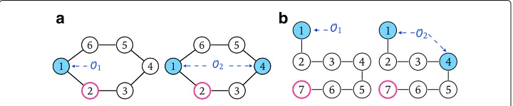
Unfortunately we cannot use a submodularity argument to give guarantees on the per-formance of Algorithm 1 because the number of equivalent classes, and hence the func-tionPs, are not submodular. Consider as a simple example a cycle of length 6 as in Fig. 6a. If the observer set isO1= {1}the number of equivalence classes isq=1. If we add node

2 toO1the classes become{1, 5, 6}and{2, 3, 4}(q = 2). Hence by adding node 2 to the

set{1}the gain in terms of equivalence classes is just 1. Consider nowO2= {1, 4} ⊇O1,

which identifies as classes{1},{4},{2, 6}and{3, 5}. If again we add node 2 toO2we reach

a DRS ofC, i.e., all classes are singletons. This means that the gain in terms of equivalence classes is 6−4 = 2 > 1 and we conclude that the number of equivalence classes is not submodular.

Comparison with benchmarks

As budgeted observer placement (even in the zero-variance setting) is NP-hard, there is no optimal algorithm to compare against. Instead, we evaluate the performance of our algorithm against a set of natural benchmarks that have shown to have good performance in other works (Seo et al. 2012; Berry et al. 2006; Zhang et al. 2016) (see “Comparison against benchmarks” section for a discussion of these benchmarks, Figs. 10-12 for the results).

Alternative objective functions. We further compare LV-OBS against two other natural heuristics that also optimize an objective function greedily.

The first is an adapted version of the approximation algorithm for the DRS problem proposed by Chen et al. (2014) and described in Appendix A.

By stopping the greedy process after it selectsknodes, we can adapt in a natural way this approximation algorithm and create a heuristic for the budgeted version that we denote by ent. We want to check if LV-OBSactually reaches smaller values of Ps compared toent.

The second is a direct minimization of the expected error distanceD =E[d(s,ˆs)] of Eq. (3) that we denote bydist. Even ifLV-OBSis not directly minimizingD, we want to

compare the results we obtain in terms ofDwith those obtain todistin order to check if, at least in some budget regimes, we can use the maximization ofPsas a proxy for the minimization ofD.

The results of our empirical evaluation are presented in Table 2 in Appendix C. The results achieved byentanddistare, on average, worse than those of Algorithm 1 both in terms ofPsand ofD, independently of the graph topology. We observe two excep-tions. First, whenkis very small:distreaches smaller values ofDcompared toLV-OBS,

which can explained by the fact thatdist directly minimizes Dand that, when fewer

The high-variance regime

When the variance is not guaranteed to be low, as defined in “The low-variance regime” section, computing analytically the success probability - or other metrics of inter-est - is unfortunately not possible (except for very simple graphs, like the path network of Fig. 2, and for particular transmission delays, e.g., Gaussian-distributed).

When the variance is high, also the localization of the source is more challenging because the observed infection delaysti−tjcan be misleading, especially if the corre-sponding observersoiandojarefarfrom the source. Take, for example, a path of length

Lwhere the two leaves are the only two observers and all edges have weight equal to 1. Figure 5a shows how the success probabilityPsdecays faster for increasing values ofL. Building on this observation, we propose a strategy for observer placement that enforces a controlled distance from a general source node to the observer set.

Source localization.For the high-variance case we localize the source using an adapted version of the algorithm proposed by Pinto et al. (2012) (see Appendix D for details). This adapted algorithm can be seen as a generalization to the high-variance regime of the source localization method presented in “Identification of the source class” section for the low-variance regime.

Observer placement

First, we formalize why distances between observers are important. Recall that for every transmission delayXuvwe assume Var(Xuv)=g(wuv,σ), withgbeing an increasing func-tion of both its arguments. Ifoi,ojare two observers connected by a unique pathP(oi,oj) and the source isv∈P(oi,oj), then

var(ti−tj)=

⎡ ⎣

uv∈P(oi,oj)

g(wuv,σ).

⎤

⎦. (6)

For example, ifXuv∼N

wuv,σ2w2uv

we have

var(ti−tj)=σ2

⎡ ⎣

uv∈P(oi,oj) w2_uv

⎤

⎦. (7)

Although we cannot controlσ, we can control thepath lengthbetween observers.

a

b

Fig. 5aSuccess probabilityPson a path of lengthLfor increasing varianceσ.bCounterexample for the

We make use of the following sufficient condition for a set to be a DRS, i.e., for an observer set to guarantee correct source localization.

Lemma 2LetG=(V,E)be a network,O⊆V . If for every u∈V there exist o1,o2∈O such that there is a unique shortest pathP(o1,o2)between o1and o2and u ∈ P(o1,o2), thenOis a DRS for G.

ProofLetu,v∈V\O. We will prove that there existo1,o2∈Osuch that the pair(u,v)

is resolved by(o1,o2), i.e.,d(v,o1)−d(u,o1) = d(v,o2)−d(u,o2). Leto1,o2 ∈ Osuch

thatuappears in the unique shortest pathP(o1,o2)ando3,o4 ∈ Ssuch thatvappears

in the unique shortest pathP(o3,o4). Ifv∈ P(o1,o2)oru ∈ P(o3,o4)thanuandvare

resolved by, respectively, (o1,o2) or (o3,o4). Takev ∈/ P(o1,o2) andu ∈/ P(o3,o4). In

this case,{o1,o2} = {o3,o4}. Let us suppose without loss of generality thato1 ∈ {/ o3,o4}.

We look only at the case where(o1,o2)does not resolve(u,v)and prove that the pair is

indeed resolved by two vertices inO. Since(o1,o2) does not resolve(u,v), there exists c ∈ Rsuch thatd(v,o1)−d(u,o1) = c = d(v,o2)−d(u,o2). Since the unique

short-est path betweeno1ando2goes throughu we have thatc > 0. We prove that either

(o1,o3)or(o1,o4)resolves(u,v). If this was not the case, we would have the following

equalities:

c=d(v,o1)−d(u,o1)=d(v,o3)−d(u,o3)

c=d(v,o1)−d(u,o1)=d(v,o4)−d(u,o4).

Sincec>0,d(v,o3) >d(u,o3)andd(v,o4) >d(u,o4)giving a contradiction withv(and

notu) being on the shortest pathP(o3,o4). We conclude that(u,v)are resolved by either

(o1,o3)or(o1,o4).

The converse of this lemma is not true: IfOdouble resolvesG, it is not even true that for every nodeuthere must existo1,o2∈Osuch thatuis contained insomeshortest path

betweeno1ando2of (see Fig. 5b).

Path covering strategy.We take Lemma 2 as a basis for deriving apath covering strat-egy for observer placement. In practice, the condition about theuniquenessof the shortest path is too strong and excludes many potentially useful observer nodes. Experimentally we see that in many practical situations two shortest paths differ only by a few nodes and the majority of nodes on the path are resolved by the two extreme nodes. This is why we relax the condition of Lemma 2 and we prefer, when the shortest path is not unique, to select one arbitrarily. LetS ⊆ V be a set of observers andLa positive integer: We call

PL(S)the set of nodes that lie on a shortest path of length at most Lbetween any two observers in the setS. Given a budgetk, and a positive integerL, we denote byS_k,Lthe set ofkvertices that maximize the cardinality ofPL(S). We callLthelength constraintfor the observer placement because we consider an observer to beusefulfor source localization only if it is within distanceLfrom another observer.S_k,L can be approximated greedily as in Algorithm 2. The running time of Algorithm 2 isO(n2k2), however, as Algorithm 1, this algorithm is highly parallelizable and hence tractable even for large networks.

We will refer to the observer placement produced by Algorithm 2 as HV-OBS(L)to

Algorithm 2(HV-OBS): Observer placement for the high-variance setting Require: NetworkG(V,E), budgetk, length constraintL

n← |G|

forv∈Vdo Ov←v

while|PL(Ov)| =nandOv<kdo

u←argmax_z∈V\Ov[|PL(Ov∪ {z})| − |PL(Ov)|] Ov←Ov∪ {u}.

returnargmax_v∈V|PL(Ov)|

Unfortunately also for Algorithm 2 we cannot use a submodularity argument to derive approximation guarantees. In fact, the functionPLis not submodular. Consider the path P of 7 nodes in Fig. 6b, fixL= 3 and setO1= {1}. If we add node 7 toO1no node lies

on a path of length smaller thanL=3 among the two observers 1 and 7, hence the gain is 0. Consider nowO2= {1, 4} ⊇O1. If we add node 7 toO2, the gain is 3 because node

5, 6 and 7, that did not lie on any path of length smaller thanLconnecting two observers before, now lie on the path connecting 4 and 7, hencePLis not submodular.

Comparison with Algorithm 1.Note that takingLequal to the maximum weighted distancebetween two nodes inGdoes not make Algorithm 2 equivalent to Algorithm 1, i.e., we do not obtainLV-OBS. To see how the two algorithms could give different results, take a cycle of odd lengthdwith a leaf node added as a neighbor to an arbitrary nodev

and assume to start the algorithm with initial set{v}. At the first step, the two algorithms will make the same choice, choosing one of the two nodes that is at distance(d−1)/2 fromv. At the second step however,LV-OBSwill add (a DRS contains all leaves (Chen et al. 2014)), whereas Algorithm 2 will add a node on the cycle. This observation is key to our results because it explains why Algorithm 2 results in a more uniform (and hence

variance-resistant) observer placement with respect toLV-OBS.HV-OBSoperates a trade-off between the average distance to the observers and the maximization ofPs.

Choice of the L parameter.How could one optimally setL? Needless to say, the opti-malLdepends on the network topology and on the available budget: Clearly, for a larger budget a smallerLis preferred.

The cardinality ofPL(O)is a good proxy for the performance ofO. The value|PL|is increasing inLand reaches its maximum forLequal to the maximum weighted distance . For smallL,|PL(HV-OBS)|<|P(LV-OBS)|but forLlarge enough this is no longer the

case. See Fig. 7a for an example. Our empirical results suggest thatLshould be chosen as the maximum for which|PL(HV-OBS)| ≤ |P(LV-OBS)|. The key property ofHV-OBS

a

b

Fig. 6Counterexamples for the submodularity property of Algorithms 1 and 2. For the graph in (a) (respectively, (b)) the gain of adding the node withred borderto_O2is larger in terms ofPs(respectively,PL)

Fig. 7Fraction of nodes inPL(·)for the California dataset with 2% of observers

with respect toLV-OBSis that observers are spread moreuniformlywithoutlosing too much in terms of success probabilityPs: Fig. 8a shows|PL(HV-OBS)|andPsas a function ofL. An a-priori evaluation of the variance threshold above which one should use the

HV-OBSplacement (and of the appropriate value of theLparameter) can be based on the

comparison ofPs on a path graph for different values ofLandσ as in Fig. 5a. In fact, looking at Fig. 5 we see that, for small values ofσPsis very close to 1 independently ofL, henceLV-OBSis the best solution. Whenσ grows, we see that, in order to guarantee an

a

b

c

d

Fig. 8Fraction of nodes inPL(HV-OBS)and success probability in the zero-variance regime (_Ps(σ=0)) as a

highPsone must choose smaller and smaller values ofL.LV-OBSandHV-OBScan give drastically different observers (see Fig. 9a for an example).

Empirical results Datasets

We purposely run our experiments on three very different real-world networks that, in addition to being relevant examples of networks for epidemic spread, display different characteristics in terms of size, diameter, clustering coefficient and average degree (see Table 1), enabling us to test the performance of our methods on various topologies.

The three networks we consider are:

Friend & Families (F & F). This is a dataset containing phone calls, SMS exchanges and bluetooth proximity, among a community living in the proximity of a university campus (Aharony et al. 2011). We select the largest connected component of individuals who took part in the experiment during its whole duration. The edges are weighted, according to the number of phone calls, SMSs, and bluetooth contacts. Facebook-like Message Exchange (FB) (Opsahl and Panzarasa 2009). As the

individuals included in this dataset were living on the same university-campus, the number of messages exchanged is likely to be a good measure of in-person interaction. We selected links on which at least one message was sent in both directions and individuals that had a contact with at least one other individual. California Road Network (CR) (California Road Network). In order to obtain a single

connected component and remove points that effectively represent the same location, we collapsed the points falling within a distance of 2 km. Moreover we iteratively deleted all leaves. In fact, the roads that cross the state border are not completely tracked in this dataset and terminate with a leaf. Some other leaves might represent remote locations, not necessarily close to the borders, but their influence on the epidemic should anyway be very low.

The diameter of the CR network is very large compared with that of the other two networks.

The edges are weighted according to a rescaled version of the real distance (measured in km).

In all three networks, edges are given (non-unit) integerweights, which is realistic in many applications as the expected transmission delays are known only up to some level of precision. Integer weights donotsimplify the localization of the source; in fact, this makes itmoredifficult to distinguish between vertices. For example, if the edges of the CR

c b

a

Table 1Displays statistics for the networks examined

|V| |E| min₍wuv) avg(wuv) max(wuv) Avg

Degree

Diameter Avg Dist Avg Clust.

Friends & Families 120 563 4 5.58 7 9.38 6 17.5 0.67

Facebook Messages 1020 6205 1 2.97 5 12.16 5 6.69 0.09

California Roads 1259 1801 1 1.71 9 2.86 66 55.3 0.2

network were weighted according to the Euclidean distance between the two endpoints,

LV-OBSwould use only a very small portion of the budget and the comparison with other

observer placements would not be meaningful.

Comparison against benchmarks

We compareLV-OBSandHV-OBSagainst the following benchmarks:

ABC (Adaptive Betweenness Centrality): Betweenness Centrality (BC) is a popular method for placing observers for source-localization (see, e.g., (Louni and

Subbalakshmi 2014) and (Seo et al. 2012), where it emerges as the best heuristic for observer placement among those tested). It consists of thek nodes having the largest BC, which is defined, for allu∈Vas

BC(u)=

x,y∈V,x=y σx,y(u)

σx,y

whereσx,yis the number of shortest paths betweenx and y andσx,y(u)is the number of those paths that passes throughu. Here we consider an adaptive version of BC (ABC) which iteratively chooses the node that maximizes the betweenness centrality without considering the shortest paths that pass by already-chosen vertices (Yoshida 2014). ABC, with respect to the basic BC, gives less clustered, and hence more efficient, observer sets.

Coverage-rate (COVERAGE) (Zhang et al. 2016): This approach maximizes the number of nodes that have an observer as a neighbor, i.e.,

C(O)= | ∪o∈ONo|/n

whereNodenotes the set of neighbors ofo. It has been shown to outperform several

heuristics with a diffusion model and a source-localization setting that are very similar to ours (Zhang et al. 2016).

K-MEDIAN: this is the optimal placement for the closely-related problem of

maximizing the detectability of a flow (Berry et al. 2006). TheK-MEDIANplacement is the set ofk nodesOsuch that

O=argmin_|O|=k

s∈V (min

o∈Od(s,o)).

Transmission delays

Unless otherwise specified, we sample the transmission delaysXuvfrom truncated Gaus-sian random variables with parameters(wuv,σwuv, [wuv/2,3wuv/2]). More precisely, if

Yuv ∼N(wuv,σwuv)is a Gaussian random variable,Xuvis obtained by conditioningYuv withYuv∈[wuv/2,3wuv/2]. With respect to the delay distribution assumed by Pinto et al. (Pinto et al. 2012) i.e.,Xuv∼N(wuv,σwuv), the distribution we assume has the advan-tage of admitting only strictly positive infection delays. Furthermore, different values of the parameterσresult in different regimes for the transmission delays, making our model very versatile. Whenσ=0, we are in the zero-variance regime; whenσis large, the distri-bution ofXuvbecomes closer to a uniform random variableU([wuv/2,3wuv/2]). Finally, whenσis strictly positive but small,Xuv ≈N(wuv,(σwuv)2).

To assess the robustness of our approach for source localization and observer place-ment, we also experiment with uniformly distributed transmission delays, i.e., for every edgeuv ∈ E, we takeXuv ∼ Unif([(1−ε)wuv,(1+ε)wuv]). The uniform distribution is, among the unimodal distributions on a bounded support, the one that maximizes the variance (Gray and Odell 1967). Hence, uniform delays are a very challenging setting for source localization.

Experimental results

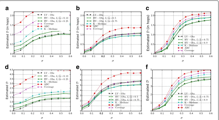
We estimate the probability of successPsand the expected distanceDfor different values of the variance parameterσ. Our estimations are computed averaging the results obtained choosing each node in turn as the source and generating synthetic epidemics. For the FB and CR datasets, we run 5 simulations per node and value ofσ; for the F & F dataset, as the network is smaller, we run 20 simulations per node and value ofσ. For the FB and CR datasets, we localize the source based on the first 20 observations only: Given the large size of these networks, it would be unrealistic to wait for all the nodes to get infected before running the algorithm.

The results forPs are displayed in Fig. 10. An approximation of the valueσ1, above

which HV-OBS outperformsLV-OBS, is marked with a vertical line. For the expected distance (weighted and in hops), see Fig. 11.

We first take as budget for the observers the minimum budget for whichPs(LV-OBS)=

1. This corresponds tok ∼ 10% for the F & F dataset, k ∼ 9% for the CR network

andk ∼ 5% for the FB dataset. This is the setting in which we expect the

improve-ment ofHV-OBSoverLV-OBSto be especially strong: For smaller values ofkwe expect

LV-OBSto be nearly optimal even in the high-variance regime because we do not have

enough budget to contrast both the topologicalundistinguishabilityamong nodes (what

LV-OBS is designed for) and the accumulation of variance (what HV-OBS is designed

for).

For the F & F and the CR networks, we also experiment with smaller percentages of observers and consistently find an improvement of HV-OBS over LV-OBS in the high-variance regime: Below a certain amount of high-variance σ1 LV-OBSperforms better than HV-OBSfor any choice of the parameterL, whereas aboveσ1a calibrated choice ofLleads

to a significant improvement. SuchLstays constant for allσ > σ1, i.e., with the notation

of Fig. 1 we haveσ1=σF.

c b

a

f e

d

Fig. 10 Success probabilityPsas the variance parameterσincreases.aCR, 2% observers.bCR, 5%

observers.cCR, 9% observers.dFB, 5% observers.eF & F, 5% observers.fF & F, 10% observers

Both LV-OBS and HV-OBS systematically outperform the baseline heuristics for

observer placement that we described in “Comparison against benchmarks” section. For the CR dataset the performance of Adaptive Betweenness Centrality is particularly poor. The Coverage Rate heuristic outperforms Adaptive Betweenness Centrality on all three networks (confirming what found by by Zhang et al. (2016)) but is consistently less effective than K-Medians and than our methods.

Finally in Fig. 12, we consider uniform transmission delays, and we measure whether, without making any changes, our observer placement still performs well. We find com-parable results which suggest that our observer placement is not dependant on the exact transmission model and that the variance of the transmission delays is really a key factor for a good observer placement.

c b

a

f e

d

c b

a

Fig. 12 Success probability_Psfor uniform transmission delaysXuv∼Unif([(1−ε)wuv,(1+ε)wuv]).aCR,

5% observers.bF & F, observers.cFB, 5% observers

Related work

The problem of source localization has been widely studied in recent years, we survey the works that are more relevant to ours and refer the reader to the survey by Jiang et al. (2014) for a more complete review of the different approaches.

Transmission delays. Many transmission models for epidemics have been studied (Lelarge 2009) and considered for source localization. Although discrete-time transmis-sion delays are common (Luo et al. 2014; Prakash et al. 2012; Altarelli et al. 2014), in order to better approximate realistic settings, much work (including ours) adopt continuous-time models with varying distributions for the transmission delays; e.g., exponential (Shah and Zaman 2011; Luo and Tay 2012) or Gaussian (Pinto et al. 2012; Louni and Subbal-akshmi 2014; Louni et al. 2015; Zhang et al. 2016). In the same line of the latter class of works, we usetruncatedGaussian variables, which gives us the advantage of ensuring that infection delays are strictly positive.

Source localization. Many approaches (Zheng and Tan 2015; Prakash et al. 2012; Sundareisan et al. 2015), beginning with the seminal work by Shah and Zaman Shah and Zaman (2011), rely on knowing the state of theentirenetwork at a fixed point in time t; this is often called acomplete observation of the epidemic. These models use maximum likelihood estimation (MLE) to estimate the source. The results of (Shah and Zaman 2011) have been extended in many ways, for example in the case of multiple sources (Luo and Tay 2012) or to obtain alocal source estimator (Dong et al. 2013). An alternate line of work considers a complete observation of the epidemic, except that the observed states arenoisy, i.e., potentially inaccurate (Zhu and Ying 2013; Sun-dareisan et al. 2015). As assuming the knowledge of the state of all the nodes is often not realistic,partial observationsettings have also been studied. In such a setting, only a subset of nodes O reveal their state. In this line of work, the observers are mainly

given, either arbitrarily or via a random process, and the problem ofselectingobservers is not addressed. For example, when a fractionxof nodes are randomly selected, Lokhov et al. (2014) propose an approach which relies on the knowledge of the state (S, I or R) of a fraction of the nodes in the graph at a given moment in time and in which the starting time of the epidemic, if unknown, can be inferred from the data available. When the nodes are independently selected to be observers, an approach to source

estimation based on the notion of Jordan center was proposed (Luo et al. 2014) and

has since been used for source estimation, especially with regard to a game theoretic

by using infection times we can achieve exact source localization in the zero-variance setting with sufficiently many observers (Chen et al. 2014), whereas this is not true otherwise.

Observer placement. Natural heuristics for observer placement (e.g., using high-degree vertices or optimizing for distance centrality) were first evaluated under the additional assumption that infected nodes know which neighbor infected them (Pinto et al. 2012). Later, Louni and Subbalakshmi (2014) proposed, for a similar model, to place the observers using a Betweenness-Centrality criterion (which we use as a benchmark, see “Comparison against benchmarks” section), and extended it to noisy observations (Louni et al. 2015). These and other heuristic approaches for observer placement are evaluated empirically by Seo et al. (2012); they reach the conclusion that, among the placements they evaluate, the Betweenness-Centrality criterion performs the best. In their work the source is estimated by ranking candidates according to their distance to the set of observers, without using the time at which the observers became infected. Once again, this approach is inherently limited by the fact that it does not make use of the time of infection.

The problem ofminimizing the number of observers required to detect the precise

source (as opposed tomaximizingthe performance given abudgetof observers) has been considered in the zero-variance setting. For trees, given the time at which the epidemic starts, the minimization problem was solved by Zejnilovic et al. (2013). Without assuming a tree topology and a known starting time, approximation algorithms have been devel-oped towards this end (Chen et al. 2014) (still in a zero-variance setting). However, in a network of size n, the number of observers required, even if minimized, can be up to n−1, hence, a budgeted setting is practically more interesting. For trees, the bud-geted placement of observers was solved by using techniques different from ours (Celis et al. 2015). However these techniques heavily rely on the tree structure of the network and do not seem to be extendible to other topologies. In a recent work, Zhang et al. (2016) consider selecting a fixed number of observers using several heuristics such as Betweenness-Centrality, Degree-Centrality and Closeness-Centrality and they show that none of these methods are satisfactory. They introduce a new heuristic for the choice of observers, calledCoverage-Rate, which is linked to the total number of nodes neighboring observers, and show that an approximated optimization of this metric yields better perfor-mance. Connecting the budgeted placement problem to the un-budgeted minimization problem, we provably outperform their approach in low-variance settings. For example, in the low-variance setting, on cycles of odd-lengthdwith budgetk =2, any two nodes at distance more than 2 are equivalent with respect to Coverage-Rate, but they maxi-mizePsonly if they are at distance(d−1)/2; our approach instead, selects this optimal placement. Moreover, the effect of the variance in the transmission delays is neglected by Zhang et al., leaving open the question of whether their approach works in general. We consider Coverage-Rate as one of our baselines.

Conclusion and future work

A direction for future work would be to measure the performance withworst caserather thanaverage casemetrics: if we can handle (adversarially chosen) source distributions where the epidemic starts at the least-observed location, then this gives a bound on the performance with anarbitrary prior distribution.

A natural extension of our model was recently studied in a work by Spinelli et al. (2017) which accounts for two stages of observation. In the first stage, as in this work, a small set of observers are selected to monitor the network. In the next stage, once an epidemic begins, additional observers are deployed in the relevant region of the network to localize the source. The latter work does not address interesting questions such as the impact of the initial budget deployed and of the position of the observers chosen in the first stage. The techniques and the results of this paper pave the way for answering these questions which we consider of high practical importance.

Endnotes

1_{A preliminary version of this work was presented at the 54}th _{Annual Allerton}

Conference on Communication, Control, and Computing (Spinelli et al. 2016).

2_{Note that in Figs. 2 and 5a we compute the value of the success probabilityPsassuming}

Gaussian distributed delays (and ignoring that, with low probability, negative delays could appear) because this is the only distribution that makes the exact computation of this value feasible. However, in all experiments we only consider non-negative distributions forXuv.

3_{See “Metrics for source localization” section for a discussion of alternative metrics for}

source localization.

4_{CallOoptthe optimal observer placement for any of the metrics considered andLthe}

leaves set. IfOoptLthere would be observero∈Ooptequivalent to a leaf /∈Ooptand by substitutingowith we would break [o] in two or more smaller equivalence classes. In this way the value of the metric considered would get closer to its optimum.

5_{The standard error of measurement is not reported for the sake of readability but it}

was checked to be small.

6_{Lyapunov condition withδ = 1 is easily verified for a sequence of independent and}

uniformly bounded random variables (see Example 27.4 in (Billingsley 1995) for more details).

7_{https://github.com/bmspinelli/observers_for_source_loc.}

Appendix A: Double Resolving Sets

The problem ofminimizingthe required number of observers in order to perfectly iden-tify the source in the zero-variance setting has been studied (Chen et al. 2014); an observer setOsuch thatPs(O)=1 is called a Double Resolving Set (DRS). While the original for-mulation of the DRS problem is slightly different, this version follows straightforwardly from our observations in “The low-variance regime” section.

Definition 3(Double Resolving Set)Given a networkG, S⊆ V is said to be a Double Resolving Set ofGif for any x,y∈ V there exist u,v∈S s.t. d(x,u)−d(x,v) =d(y,u)− d(y,v).

function, has been studied. Note that this has no connection to true information-theoretic entropy.

Definition 4(Entropy (Chen et al. 2014))LetG a network,O ⊆ V ,|O| = k a set of observers. The entropy ofOis

H_O=log₂

⎛ ⎝

[u]O⊆V |[u]_O|!

⎞ ⎠

Note thatH_O is minimized if and only if each equivalence class consists of only one

node and hence if and only if Ps = 1. However, despite the fact that H_O is

mini-mized whenPs is maximized and that both act on the same set of equivalence classes

for a given O, the greedy processes that minimizeH_O and maximize Ps are not the

same. This can be seen by rewriting both objective functions in the following way. Let [c1,. . .,cq] be the sequence of equivalence class sizes. ThenHO can be written as

H_O([c1, ..,cq]) = li=1 ci

j=2log(j) = maxcj

i=2 log(i)#{cj ≥ i}. Analogously we have the following equality for the success probabilityPs([c1,. . .,cq]):n(1−Ps([c1,. . .,cq]))=

n−q=max_i=2cj#{cj≥i}

Hence, though similar in spirit, a greedy minimization ofHO is not related to a greedy optimization ofPs(orE[d(s∗,ˆs)]).

Appendix B: Hardness of Budgeted Observer Placement

Theorem 3Given a networkG=(V,E)and a budget k, finding an observer setOwhich maximizesPsis NP-hard.

ProofWe will prove that the budgeted observer placement is NP-hard with a reduc-tion from the DRS problem (see Appendix A: Double Resolving Sets secreduc-tion), i.e., given a polynomial-time algorithm for the budgeted observer placement problem, we will prove that we can solve the DRS problem in polynomial time.

Assume that we have a polynomial-time algorithmA that takes as input a network

G=(V,E)and a budgetk, and outputs a setO⊆Vof sizeksuch thatPsis maximized. Recall from “The low-variance regime” section that given a networkGand a setO, the probabilityPscan be calculated in timeO(n)wheren= |V|(it is enough to compute the

ndistances vector with respect toOand any reference observero1∈O). Hence, we will

construct an algorithm for the DRS problem.

Algorithm 3Finds the minimum cardinality DRS given an algorithm to compute the

k-nodes set that maximizesPs Require: NetworkG=(V,E)

fork=1,. . .,|V|do O:=A(G,k) P:=Ps(O) ifP=1then

Since the full setV always resolves the network, the program is well defined (i.e., it always returnssome k). Moreover, it returns precisely the minimum budgetkrequired in order to attainPs=1. Lastly, it is clear that the runtime is at mostO(n(p_A(n)+n))where

p_A(n)is the running time of algorithmA. Hence, we have a polynomial-time algorithm for the DRS problem.

Appendix C: Alternative objective functions for Algorithm 1

We present the results of the experiment described in Comparison with benchmarks section. Let us here denoteLV-OBSwithfor consistency of notation.

Table 2 comparesLV-OBS,entanddist, for different topologies and different budgets

k, in terms of both Ps andD. The results are given in the form of (averaged) relative differences.5

We denote the relative difference ofxandywith respect tof as

ρ(f,x,y)def= f(y)−f(x) f(x) .

Since the expected distance can be equal to 0 we add 1 to the denominator when comparing values ofD, i.e.,

ρ(D,x,y)def= D(y)−D(x)

D(x)+1 .

Appendix D: Source Localization in the High-Variance Regime

We describe here how we compute the estimated sourcesˆin the high-variance regime. Denote byT_O the vector of the observed infection times. If the transmission delays are Gaussian-distributed,Gis a tree, the maximum likelihood (ML) estimator defined as

ˆ

s∈arg max

s∈V P(s|TO),

has a tractable closed form (Pinto et al. 2012). Note that the model of (Pinto et al. 2012) additionally assumed infected observers knew the neighbor that infected them; this assumption is not essential for the derivation of the ML estimator and it is not required in our work.

In particular, given a set of observers

O= {o1,o2,. . .,ok} ⊆V,

Table 2Comparison ofLV-OBS() with the greedy algorithms that minimize the entropy function of (Chen et al. 2014) (ent) and the expected distance (dist)

ρ(Ps,,dist) ρ(D,dist,) ρ(Ps,,ent)

Random Geometric Network,N=100,r=0.2

k=2 -0.205 0.101 -0.033

k=4 -0.014 -0.003 -0.007

k=8 -0.003 -0.002 -0.003

Barabàsi Albert Network,N=100,m=3

k=2 -0.168 0.023 -0.037

k₌4 -0.039 0.025 -0.028

the vector of the observed infection delaysτ =[t2−t1,. . .,tk−t1]∈Rk−1is distributed as

N(ds,o1,O)whereds,o1 is the distance vector of Definition 2 and the covariance matrix

o1is

o1,(k,i)=σ

2 (u,v)∈P(o1,ok+1)w 2

uv k=i

(u,v)∈P(o1,ok+1)∩P(o1,oi+1)w 2

uv k=i,

(8)

withP(x,y)denoting the set of edges in the unique path betweenxandy. Hence the ML estimator is

ˆ

s ∈arg max_s∈V exp

−1 2

τ−ds,o₁o₁−1

τ−ds,o₁

|o₁|1/2

=arg maxs∈V

d_so₁−1τ −1₂ds,o1 .

(9)

On non-tree networks, the multiplicity of paths linking any two nodes makes source estimation more challenging. As claimed in (Pinto et al. 2012), the same estimator can be used as an approximation of the ML estimator for a non-tree network by assuming that the diffusion happens only through a BFS (Breadth-First-Search) tree rooted at the (unknown) source. In this case the paths which appear in the definition of the covariance

matrixo₁ are computed on the BFS tree rooted at the candidate source considered.

Henceo₁depends on the candidate source and the ML estimator is

ˆ

sBFS∈arg max

s∈V

exp−1₂(τ−ds,o1)so1

−1_(τ−d

s,o1)

s o1

1/2

. (10)

In this work, we adopt (10) as the source estimator in the noisy case. In fact, even if our edge delays are not Gaussian-distributed, under the hypothesis of sparse observa-tions, we can apply the Central Limit Theorem (CLT) to approximate the sum of the edge delays with Gaussian random variables: if all edges have the same weight we can apply the CLT for i.i.d. random variables; if this is not the case, we can apply Lyapunov’s ver-sion of CLT.6Using (10) to compute the ML estimator, the likelihood of nodes in the same equivalence class can result to be different as an artefact of the BFS-tree approximation. Hence, for consistency with our source-localization method in the low-variance case, we compute an average likelihood and estimate that the source is in the class with the higher average likelihood. Then, once an equivalence class for the source is estimated, we selectˆs

by sampling the prior probability on the position of the source (if available) or by uniform sampling from the estimated equivalence class.

Acknowledgements

The authors wish to thank the anonymous reviewers for their helpful comments and suggestions. B. Spinelli was partially supported by the Bill & Melinda Gates Foundation, under Grant No. OPP1070273.

Availability of data and materials

The datasets and the code used for all the experiments presented in this section are publicly available on GitHub.7

Authors’ contributions

All authors participated in the conception and design of the work. BS prepared the experimental setup, analysed the experimental results and drafted the manuscript. All authors participated in a critical revision of the manuscript and approved it in its final form. All authors read and approved the final manuscript.

Competing interests

The authors declare that they have no competing interests.

Publisher’s Note