R E S E A R C H
Open Access
A global model of avian influenza prediction in
wild birds: the importance of northern regions
Keiko A Herrick
1, Falk Huettmann
1,2*and Michael A Lindgren
3Abstract
Avian influenza virus (AIV) is enzootic to wild birds, which are its natural reservoir. The virus exhibits a large degree of genetic diversity and most of the isolated strains are of low pathogenicity to poultry. Although AIV is nearly ubiquitous in wild bird populations, highly pathogenic H5N1 subtypes in poultry have been the focus of most modeling efforts. To better understand viral ecology of AIV, a predictive model should 1) include wild birds, 2) include all isolated subtypes, and 3) cover the host’s natural range, unbounded by artificial country borders. As of this writing, there are few large-scale predictive models of AIV in wild birds. We used the Random Forests algorithm, an ensemble data-mining machine-learning method, to develop a global-scale predictive map of AIV, identify important predictors, and describe the environmental niche of AIV in wild bird populations. The model has an accuracy of 0.79 and identified northern areas as having the highest relative predicted risk of outbreak. The primary niche was described as regions of low annual rainfall and low temperatures. This study is the first global-scale model of low-pathogenicity avian influenza in wild birds and underscores the importance of largely unstudied northern regions in the persistence of AIV.
Introduction
The influenza viruses that caused the four deadliest hu-man pandemics of the past century (1918, 1957, 1968, 2009) contained gene segments from avian influenza ac-quired through recent reassortment events (reviewed in [1]). Influenza is thought to have originated in wild birds, and waterfowl are considered the primary reser-voir. Avian influenza virus (AIV) most commonly infects Anseriformes,Passeriformes, andCharadriiformesin wild populations, particularly family Anatidae[2]. The Asian strains of the highly pathogenic H5N1 AIV subtype in poultry have received the most attention because of eco-nomic losses caused by this subtype, the virus’s transmis-sibility from chicken to human [3,4], and fears over a new human influenza pandemic [5]. However, HPAI H5N1 is not the only strain with pandemic potential: cases of human infection with interspecies H7 and H9 subtypes have been reported [6,7] and others, such as
H6, can be highly pathogenic to poultry. The vast majo-rity of influenza strains are of low pathogenicity to poultry, but because AIV is a virus of great diversity with the potential for rapid evolution [8], the full range of its variation should be considered rather than just focusing on a single strain or subtype. A massive reservoir of ge-netic diversity for potential reassortment of AIV exists in wild bird populations, from which nearly all combina-tions of hemagglutinin (H) and neuraminidase (N) sub-types have been isolated [9-11].
A number of ongoing surveillance projects record the subtypes of AIV isolated from wild birds [9,10,12,13]. Large cooperative databases, such as the Influenza Re-search Database (IRD), curate the surveillance efforts of multiple institutions. IRD provides an opportunity to apply predictive modeling to AIV on a global scale. In the prediction and risk assessment of infectious diseases, geographic information systems (GIS) and predictive modeling techniques are important tools [14]. Predictive models of Chagas disease [15], malaria [16], leishmania-sis [17], and Lyme disease [18] have been used to map disease prevalence and identify important factors con-tributing to risk. Several models have assessed risk fac-tors for H5N1 in domestic poultry and produced high resolution models for India [19], Vietnam [20], and * Correspondence:fhuettmann@alaska.edu
1Ecological Wildlife Habitat Analysis of the Land- and Seascape (EWHALE) Lab, Biology and Wildlife Department, University of Alaska Fairbanks, Fairbanks, AK 99775, USA
2
Institute of Arctic Biology, University of Alaska Fairbanks, Fairbanks, AK 99775-7000, USA
Full list of author information is available at the end of the article
China [21]. One predictive map of multiple species of wild birds and subtypes of AIV was developed for the continental United States [22], and one for flyways adja-cent to the Pacific Rim [23].
As of this writing, there are no global-scale predictions of LPAI in wild birds. The development of a global model could be an important tool in the management and risk assessment of AIV in the interest of public and animal health. Our model extends the value of AIV sur-veillance efforts by using the data for predictive pur-poses, not simply for descriptive purposes. In addition, a global model encompasses the distribution range of im-portant reservoir species, many of which travel vast dis-tances [24] in cross-continental migratory journeys to and from breeding grounds each year. We used ensem-ble data-mining machine-learning methods to 1) identify important predictor variables, 2) quantitatively describe the environmental niche of AIV in wild bird populations, and 3) develop a near-global-scale predictive map (ex-cluding Antarctica) of AIV based on this described niche.
Materials and methods Wild bird data
Sample data points of AIV-negative and AIV-positive data for wild birds were obtained from the Influenza Re-search Database online [25]. This dataset spans five years (2005–2010) of surveillance data providing geo-referenced collection coordinates for each sample, spe-cies name, AIV-positive or–negative status (determined by the collecting institution), viral subtype (where avail-able), and many other collection specifics. We did not distinguish between high- and low-pathogenicity AIV strains in our dataset. We groomed the database to re-move samples from domestic species and samples from unidentified species (listed as “Unknown”). In addition, this version of the database contained many instances where the latitude and longitude values were inverted; we examined each point for a match between GPS coor-dinates and collection location, and corrected it if the error was obvious or removed it if uncertainty remained. We randomly divided the data points into two pools for training the model (47 898 points) and testing the model (12 080 points) using MS Excel and imported both sets as point layers into ArcMap v.10.0 (Esri, Redlands USA).
Environmental variable layers
Forty-one predictor variable layers for ArcGIS were ac-quired from open source projects and included biocli-matic, geographic, and anthropogenic variables (Table 1). The extent of this model is bounded by these data layers, which exclude Antarctica. Bioclimatic vari-ables included mean temperature for each month, for quarters (e.g. wettest quarter), and annual means for
precipitation and temperature. A number of time-dependent variables were included (i.e. mean tempe-rature in January - December) and were manipulated in order to maintain their relevance to collection locations in the Southern Hemisphere. For points with negative latitude values, time-dependent variables were shifted by 6 months, such that months were correctly associated with the austral seasons. Geographic variables included elevation, which has been identified as an important fac-tor in other AIV models [19], and lakes, rivers, and wet-lands, which are important to waterfowl. We calculated some layers from existing predictor variables using the Spatial Analyst Tool in ArcMap. The distances from fresh water features and coastline were calculated using the Euclidean Distance Tool. Slope was calculated from elevation and aspect was in turn calculated from slope. Anthropogenic variables included indices of human ma-nipulation, infrastructure, and population density. Due to the importance of chickens and pigs in the transmis-sion of AIV to humans, we included predicted poultry and pig densities [26,27]. Not all layers included Antarc-tica, so the entire continent was excluded from the study area (layers trimmed at −57° latitude) to prevent biases in calculation. We then used the Geospatial Modeling Environment (GME; [28]) to intersect, or extract the values of the predictor variables at the same geographic coordinates as the sample data points. GME adds the values of each predictor variable to the database as an additional column. The intersected database is then imported into ArcMap for visualization. Layers and metadata are stored at and can be obtained from the Ecological Wildlife Habitat Analysis of the Land- and Seascape (EWHALE) Lab at the University of Alaska Fairbanks (UAF).
Defining the outbreak niche
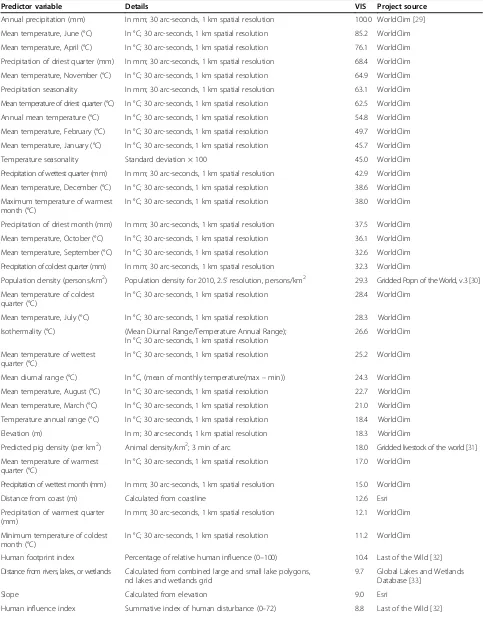
up-Table 1 The predictor variables used by the Random Forests algorithm to create a global prediction map for avian influenza virus in wild birds.
Predictor variable Details VIS Project source
Annual precipitation (mm) In mm; 30 arc-seconds, 1 km spatial resolution 100.0 WorldClim [29]
Mean temperature, June (°C) In °C; 30 arc-seconds, 1 km spatial resolution 85.2 WorldClim
Mean temperature, April (°C) In °C; 30 arc-seconds, 1 km spatial resolution 76.1 WorldClim
Precipitation of driest quarter (mm) In mm; 30 arc-seconds, 1 km spatial resolution 68.4 WorldClim
Mean temperature, November (°C) In °C; 30 arc-seconds, 1 km spatial resolution 64.9 WorldClim
Precipitation seasonality In mm; 30 arc-seconds, 1 km spatial resolution 63.1 WorldClim
Mean temperature of driest quarter (°C) In °C; 30 arc-seconds, 1 km spatial resolution 62.5 WorldClim
Annual mean temperature (°C) In °C; 30 arc-seconds, 1 km spatial resolution 54.8 WorldClim
Mean temperature, February (°C) In °C; 30 arc-seconds, 1 km spatial resolution 49.7 WorldClim
Mean temperature, January (°C) In °C; 30 arc-seconds, 1 km spatial resolution 45.7 WorldClim
Temperature seasonality Standard deviation × 100 45.0 WorldClim
Precipitation of wettest quarter (mm) In mm; 30 arc-seconds, 1 km spatial resolution 42.9 WorldClim
Mean temperature, December (°C) In °C; 30 arc-seconds, 1 km spatial resolution 38.6 WorldClim
Maximum temperature of warmest month (°C)
In °C; 30 arc-seconds, 1 km spatial resolution 38.0 WorldClim
Precipitation of driest month (mm) In mm; 30 arc-seconds, 1 km spatial resolution 37.5 WorldClim
Mean temperature, October (°C) In °C; 30 arc-seconds, 1 km spatial resolution 36.1 WorldClim
Mean temperature, September (°C) In °C; 30 arc-seconds, 1 km spatial resolution 32.6 WorldClim
Precipitation of coldest quarter (mm) In mm; 30 arc-seconds, 1 km spatial resolution 32.3 WorldClim
Population density (persons/km2) Population density for 2010, 2.5’resolution, persons/km2 29.3 Gridded Popn of the World, v.3 [30] Mean temperature of coldest
quarter (°C)
In °C; 30 arc-seconds, 1 km spatial resolution 28.4 WorldClim
Mean temperature, July (°C) In °C; 30 arc-seconds, 1 km spatial resolution 28.3 WorldClim
Isothermality (°C) (Mean Diurnal Range/Temperature Annual Range); In °C; 30 arc-seconds, 1 km spatial resolution
26.6 WorldClim
Mean temperature of wettest quarter (°C)
In °C; 30 arc-seconds, 1 km spatial resolution 25.2 WorldClim
Mean diurnal range (°C) In °C, (mean of monthly temperature(max–min)) 24.3 WorldClim Mean temperature, August (°C) In °C; 30 arc-seconds, 1 km spatial resolution 22.7 WorldClim
Mean temperature, March (°C) In °C; 30 arc-seconds, 1 km spatial resolution 21.0 WorldClim
Temperature annual range (°C) In °C; 30 arc-seconds, 1 km spatial resolution 18.4 WorldClim
Elevation (m) In m; 30 arc-seconds, 1 km spatial resolution 18.3 WorldClim
Predicted pig density (per km2) Animal density/km2; 3 min of arc 18.0 Gridded livestock of the world [31]
Mean temperature of warmest quarter (°C)
In °C; 30 arc-seconds, 1 km spatial resolution 17.0 WorldClim
Precipitation of wettest month (mm) In mm; 30 arc-seconds, 1 km spatial resolution 15.0 WorldClim
Distance from coast (m) Calculated from coastline 12.6 Esri
Precipitation of warmest quarter (mm)
In mm; 30 arc-seconds, 1 km spatial resolution 12.1 WorldClim
Minimum temperature of coldest month (°C)
In °C; 30 arc-seconds, 1 km spatial resolution 11.2 WorldClim
Human footprint index Percentage of relative human influence (0–100) 10.4 Last of the Wild [32] Distance from rivers, lakes, or wetlands Calculated from combined large and small lake polygons,
nd lakes and wetlands grid
9.7 Global Lakes and Wetlands Database [33]
Slope Calculated from elevation 9.0 Esri
weight the smaller number of AIV-positive samples against AIV-negative samples; the number of trees was set to 500; and seven predictors were used at each node [34].
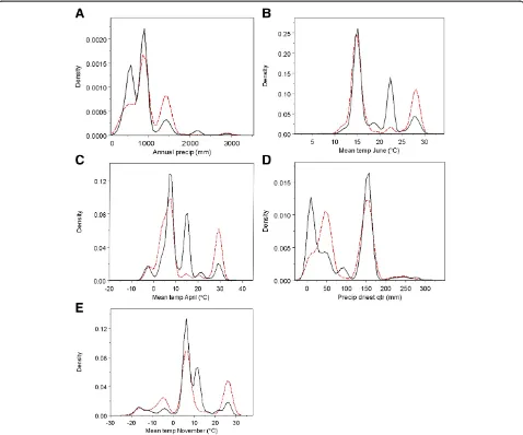
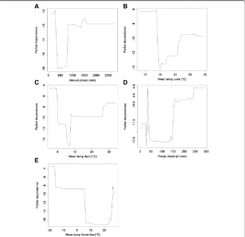
The top five variables with the highest VIS were chosen for further examination. To compare the number of AIV-positive and -negative samples taken across each variable’s range of values we plotted density using Spotfire S+ (TIBCO, v.8.2, Palo Alto USA). The ranges within which peaks occur suggest underlying mecha-nisms, which may be driving AIV outbreaks. Partial de-pendence plots were produced using the “partialPlot()” command in the RandomForest package [37] in R sta-tistical programming language [38]. Partial dependence can be thought of as an index summarizing the quan-tified relationship of a predictor with the response variable after averaging the noise of non-relevant pre-dictors [39]. Partial dependence plots can be useful in illustrating general trends in model accuracy’s depen-dence on predictors. The partial dependepen-dence of a variable’s effect is best understood by examining gen-eral patterns in relation to the values of the predictor variable rather than the specific values of partial dependence.
As a negative control, we calculated AUC for the AIV-positive status of the training subset against three individual predictors: the predictor with the highest importance score, the lowest importance score, and Annual Mean Temperature. We examined partial de-pendence plots for the general relationship between the range of predictor values and AIV-positivity (e.g. Figure 1a for Annual Precipitation). Predictor values for each point in the subset of training data were nor-malized between 0 and 1. If the relationship was nega-tive, then the values were inverted such that low values of the variable predicted high occurrence. All three sets of normalized values were then subjected to AUC calculations.
Predictive map
To predict the relative occurrence of AIV in unsampled areas, we applied the model to a lattice of points spaced 100 km apart and calculated a predicted value for each point. Random Forests expresses the predicted occur-rence of AIV as a Relative Occuroccur-rence Index (ROI)
rather than a probability score [40]. In ArcMap, we ap-plied the Inverse Distance Weighted Tool (IDW) to interpolate these ROI values between the points, and generated a map of predicted AIV outbreak locations. The final map was projected as Robinson (sphere) with the central meridian at 145° so that Africa and Europe are displayed intact.
To evaluate the performance of the model, we calcu-lated the Receiver Operating Characteristic (ROC) curve by plotting true positive points (AIV-positive sta-tus) against false positives with the program ROC_AUC [41]. A ROC value of 0.5 means a model accuracy of 50% in predicting positives and is no bet-ter than the random assignment of positive or negative status. A ROC value of 1.0 shows the model accurately classified 100% of points. If the area under the resulting curve (AUC) exceeds the critical value of 0.7, the model has high predictive power [42]. To evaluate accuracy, the model was applied to the pool of testing points. A ROC curve was calculated for these points using their predicted ROI value against their experi-mental AIV-positive status.
Results
Important predictor variables
Annual precipitation, mean temperature in June, and mean temperature in April were the most important predictor variables with VIS of 100, 85.2, and 76.1, re-spectively. Predictor variables with VIS above 50 were split almost equally between precipitation measurements and the mean temperatures in November, the driest quarter (3 month period), and annual mean temperature (Table 1). In the density plots (Figure 1a-e) the relative frequency of sampling was approximated by the dens-ity of the AIV-negative group of samples (represented by the solid black line); the range of values over which sampling occurred was inferred from the AIV-negative group. In general, the lack of perfect correspondence between AIV-positive (dotted red line) and AI–negative groups showed that there were unequal densities of positivity across the sampling range. Thus AIV-positive samples did not occur at the same relative frequency as sampling effort. The ranges where the density of AIV-positive samples exceeded those of AIV-negative samples imply conditions correlated with Table 1 The predictor variables used by the Random Forests algorithm to create a global prediction map for avian influenza virus in wild birds.(Continued)
Predicted poultry density (per km2) Animal density/km2; 3 min of arc 7.9 Gridded livestock of the world [31]
Aspect positive degrees from 0 to 359.9, measured clockwise from north; calculated from slope
6.7 Esri
Mean temperature, May (°C) In °C; 30 arc-seconds, 1 km spatial resolution 5.4 WorldClim
AIV-positivity. In the case of annual precipitation (Figure 1a), moderate (1400 mm) and very low (~0 mm) values were correlated with AIV-positivity. The partial dependence of AIV-positivity on annual precipitation exhibited a similar trend: very high de-pendence at 0 mm, a trough, and then moderately high dependence at values over 1000 mm (Figure 2a). These patterns imply that areas of low annual precipi-tation are most correlated with AIV-positivity, although areas of relatively high annual precipitation show some correlation as well. Areas of very low and high mean temperatures in June and April were correlated with AIV-positivity (Figures 1b,c), while areas of moderate temperature were not. June and April displayed similar patterns with a strong peak at the high range of sam-pling (~28°C and 30°C, respectively) and at the lowest
ranges (~10°C and 0°C, respectively). Examination of partial dependence revealed that AIV-positivity was high at the lowest temperatures, dropped sharply at moderate temperatures, and gradually increased at the higher end of the range (Figures 2b,c). Thus areas with low temperatures in June and April were correlated with AIV-positive samples. Precipitation of the driest quarter displayed one peak at 50 mm where AIV-positives had a higher density than AIV-negatives (Figure 1d). However, while the partial dependence was high at this value, it appears as a lone spike in an area of low partial dependence. Partial dependence on precipitation increases above 150 mm and reaches high levels above 250 mm (Figure 2d). While the highest density of AIV-positives occurred at relatively low annual precipitation, partial dependence was
highest at the highest range during the driest quarter, which may reflect a low seasonality or variation in rainfall during the year. Mean temperature in Novem-ber was correlated with AIV-positivity at low and high values (Figures 1e and 2e). Highest partial de-pendence occurred at the lowest ranges (< −20°C). Based on the important predictor variables, the niche of AIV-positive samples in this study was described as re-gions of low annual rainfall and low temperatures.
There appears to be a secondary niche that described regions of high precipitation and higher temperatures.
Ecological niche model
Random Forests produced a robust ecological niche model for AIV in wild birds and identified important predictor variables. The model had an ROC/AUC of 0.79 on the training points and 0.76 on the testing points, lending high confidence to its prediction of the
relative occurrence of AIV in wild birds on a global scale. The negative control test was performed by calcu-lating AUC for the training subset against Annual Pre-cipitation (the highest scoring predictor, AUC = 0.59), Mean Temperature in May (the lowest scoring predictor, AUC = 0.47), and Annual Mean Temperature (AUC = 0.47). Although Annual Precipitation received a higher AUC value than the other predictors, this AUC still did not reach the acceptability threshold of 0.7, demonstrat-ing that individual variables were poor predictors of AIV. Northern areas had the highest values of Relative Occurrence Index and temperate regions had the lowest (Figure 3). Interestingly, an equatorial band of relatively high predicted occurrence was observed, which may re-flect regions characterized by the secondary niche.
Discussion
While much of AIV modeling has focused on low-latitude regions and HPAI H5N1, we demonstrated that northern regions are important when all strains of AIV and wild reservoir species are taken into account. By cre-ating a global-scale model, we identified important areas of high predicted occurrence that were missed by AIV models for temperate and sub-tropical regions. Small, local models are vital developing strategies for managing acute outbreaks
of specific diseases. However, a global scale perspective is necessary for AIV because, unlike other diseases, is carried by a host that is capable of migrating long distances and potentially infecting others along its path. Furthermore, a model that excludes wild birds, which are the natural reser-voir for the virus, neglects the source of gene segments for future infections and potential pandemic strains.
Our model represents the first global-scale predictive map of AIV in wild birds. Using available global AIV data, we identified northern areas as having the highest relative predicted risk of outbreak. Important predictor variables included low temperatures and low annual pre-cipitation. Cold winters and low rainfall may represent con-tinental climates at high latitudes. Areas with these types of climatic conditions include landscapes in Siberia, the Rus-sian Far East, Mongolia, and northern Canada, all of which had high indices of relative occurrence of AIV. Similar con-ditions at lower latitudes may be created by high elevation, such as the climate of the Tibetan Plateau, which also had a high score. The partial dependence of AIV-positivity on rainfall was bimodal and peaked at very low and high values. This apparently contradictory finding that extremes in rain-fall were correlated with AIV-positivity may be explained through laboratory studies of transmission and persistence of the virus. Aerial, non-contact transmission of influenza between guinea pigs was most efficient below 35% relative
humidity [43]; thus, we expect dry climate to be condu-cive to the aerial spread of virus. At low relative humidity and temperature (~6°C, < 46% rh), virus persisted over two weeks on metal, glass, and in soil [44]. Wet condi-tions and low temperatures were also conducive to viral persistence: the virus remains viable nearly ten times longer in 17°C water than 28°C water [45]. At low temperatures and high relative humidity (~7°C, ~88% rh), the virus persisted over two weeks in chicken feces [44]. Low temperature is the common factor in these studies. While low relative humidity contributes to transmission and per-sistence on smooth surfaces, the virus also remains viable in water and damp materials such as bird feces. As the virus is transmitted efficiently in water, either through the fecal-oral route [46] or via tracheal shedding [47], dabbling ducks (such asAnatidae) in cool northern regions may be at in-creased risk of contracting AIV from the environment.
Our findings differed from other AIV models in the importance and range of anthropogenic variables. In our model, anthropogenic factors were represented by hu-man population density as well as the Huhu-man Influence Index and the Human Footprint Index [32], which are indices calculated based on human population density, land transformation, transportation infrastructure, and electrical power infrastructure. All the anthropogenic variables received very low VIS with human population density scoring the highest at 29.3. Previous models identified high human population density and high farm-ing intensity (especially rice croppfarm-ing and aquaculture) as important predictors [19,20,48]. The niche they de-scribed is characterized as having a high human popula-tion, high level of anthropogenic disturbance, and the high annual temperature and humidity of the sub-tropical climates for which the models were designed (i.e. Bangladesh, Vietnam, and Thailand). However, these studies were specific to HPAI H5N1 in poultry. While the one North American model in wild birds identified low minimum temperatures, with which our model was consistent, they also identified the amount of cropland as an important factor [22]. In general, our model did not predict high occurrence of AIV in the continental United States when compared to northern regions, which have not been modeled previously.
Our model demonstrated a novel use of surveillance data that goes beyond the yearly reporting of infected species and viral subtypes isolated. The application of environmental data, GIS, and machine-learning extends the usefulness of surveillance results. However, the pre-diction of relative occurrence presented here is not a final, definitive map of avian influenza in wild birds, but rather an initial attempt that demonstrates that a useful signal can be gleaned from the noise found in a global dataset. Indeed, it serves to highlight shortcomings in available data. In particular, nearly all data were collected
in the Northern Hemisphere. In addition, this Northern Hemispheric niche could then be tested on southward-migrating birds to see if the same predictions are appli-cable. A predominance of Anatidaecould create a spatial bias for northern regions and a temporal bias for summer months if most sampling is carried out during summer breeding season at high latitudes. However, if one uses the mean temperature in November as a proxy for latitude, there appears instead to be a strong temperate bias in col-lection with AIV-positive peaks occurring to either side. The bifurcate niche evident here is an interesting topic for future analysis. The mechanisms responsible for this niche require further investigation in order to clarify how the im-portant bioclimatic variables contribute to AIV-positivity.
While ongoing surveillance is important to under-standing the dynamics of AIV, efforts should include wil-derness areas, such as Siberia, that have received less attention. Models such as this one could receive add-itional fine-tuning if these results were to guide future sampling efforts in regions of high predicted occurrence, much of which remains unsampled. As both AIV-positive and AIV-negative data are incorporated into this model, all results from prediction-guided sampling strengthen the prediction, even if only a small percent-age of AIV-positive samples are isolated. Given the sheer quantity of data collected by long term surveillance ef-forts, an unprecedented opportunity exists to produce future models of greater accuracy. If data were curated and publically available, models could be treated as transparent, replicable science experiments. Improved global scale models could not only increase the under-standing of viral ecology, but also serve to guide the management of influenza risk policy for the benefit of public health on a global scale. A global model of AIV must be a collaborative effort and we hope this initial attempt encourages greater cooperation and data-sharing among members of the AIV research community.
Competing interests
The authors declare that they have no competing interests.
Authors’contributions
KH carried out the research and the manuscript preparation. ML provided expertise in data analysis. FH was involved in critical review of the manuscript and gave final approval of the version to be published. All authors read and approved the final manuscript.
Acknowledgements
Author details 1
Ecological Wildlife Habitat Analysis of the Land- and Seascape (EWHALE) Lab, Biology and Wildlife Department, University of Alaska Fairbanks, Fairbanks, AK 99775, USA.2Institute of Arctic Biology, University of Alaska Fairbanks, Fairbanks, AK 99775-7000, USA.3Scenarios Network for Alaska and Arctic Planning, University of Alaska Fairbanks, Fairbanks, AK 99775, USA.
Received: 27 August 2012 Accepted: 28 May 2013 Published: 13 June 2013
References
1. Garten RJ, Davis CT, Russell CA, Shu B, Lindstrom S, Balish A, Sessions WM, Xu X, Skepner E, Deyde V, Okomo-Adhiambo M, Gubareva L, Barnes J, Smith CB, Emery SL, Hillman MJ, Rivailler P, Smagala J, de Graaf M, Burke DF, Fouchier RA, Pappas C, Alpuche-Aranda CM, López-Gatell H, Olivera H, López I, Myers CA, Faix D, Blair PJ, Yu C,et al:Antigenic and genetic characteristics of swine-origin 2009 A(H1N1) influenza viruses circulating in humans.Science2009,325:197–201.
2. Stallknecht DE, Brown JD:Wild birds and the epidemiology of avian influenza.J Wildl Dis2007,43:S15–S20.
3. Subbarao K, Klimov A, Katz J, Regnery H, Lim W, Hall H, Perdue M, Swayne D, Bender C, Huang J, Hemphill M, Rowe T, Shaw M, Xu X, Fukuda K, Cox N:
Characterization of an avian influenza A (H5N1) virus isolated from a child with a fatal respiratory illness.Science1998,279:393–396. 4. Kandun IN, Wibisono H, Sedyaningsih ER, Yusharmen Hadisoedarsuno W,
Purba W, Santoso H, Septiawati C, Tresnaningsih E, Heriyanto B, Yuwono D, Harun S, Soeroso S, Giriputra S, Blair PJ, Jeremijenko A, Kosasih H, Putnam SD, Samaan G, Silitonga M, Chan KH, Poon LL, Lim W, Klimov A, Lindstrom S, Guan Y, Donis R, Katz J, Cox N, Peiris M,et al:Three Indonesian clusters of H5N1 virus infection in 2005.N Engl J Med2006,355:2186–2194. 5. Ligon BL:Avian influenza virus H5N1: a review of its history and
information regarding its potential to cause the next pandemic.Semin Pediatr Infect Dis2005,16:236–335.
6. Peiris JSM, de Jong MD, Guan Y:Avian influenza virus (H5N1): a threat to human health.Clin Microbiol Rev2007,20:243–267.
7. Centers for Disease Control:Avian influenza A virus infections of humans. http://www.cdc.gov/flu/avian/gen-info/avian-flu-humans.htm.
8. Suarez DL:Evolution of avian influenza viruses.Vet Microbiol2000,74:15–27. 9. Munster VJ, Baas C, Lexmond P, Waldenström J, Wallensten A, Fransson T,
Rimmelzwaan GF, Beyer WE, Schutten M, Olsen B, Osterhaus AD, Fouchier RA:Spatial, temporal, and species variation in prevalence of influenza A viruses in wild migratory birds.PLoS Pathog2007,3:630–638.
10. Krauss S, Walker D, Pryor SP, Niles L, Chenghong L, Hinshaw VS, Webster RG:
Influenza A viruses of migrating wild aquatic birds in North America.
Vector Borne Zoonotic Dis2004,4:177–189.
11. Webster R, Bean W, Gorman O, Chambers T, Kawaoka Y:Evolution and ecology of influenza A viruses.Microbiol Rev1992,56:152–179. 12. Parmley J, Lair S, Leighton FA:Canada's inter-agency wild bird influenza
survey.Integr Zool2009,4:409–417.
13. CEIRS:Centers of Excellence for Influenza Research and Surveillance (CEIRS)”. National Institute of Allergy and Infectious Diseases.http://www.niaid.nih.gov/ labsandresources/resources/ceirs/Pages/default.aspx].
14. Peterson AT:Ecologic niche modeling and spatial patterns of disease transmission.Emerg Infect Dis2006,12:1822–1826.
15. Peterson AT, Sanchez-Cordero V, Beard CB, Ramsey JM:Ecological niche modeling and potential reservoirs for Chagas disease.Mexico Emerg Infect Dis2002,8:662–667.
16. Moffett A, Shackelford N, Sarkar S:Malaria in Africa: vector species’niche models and relative risk maps.PLoS One2007,2:e824.
17. Peterson AT, Vieglais DA, Andreasen JK:Migratory birds modeled as critical transport agents for West Nile Virus in North America.Vector Borne Zoonotic Dis2003,3:27–37.
18. Mak S, Morshed M, Henry B:Ecological niche modeling of lyme disease in British Columbia, Canada.J Med Entomol2010,47:99–105.
19. Adhikari D, Chettri A, Barik SK:Modelling the ecology and distribution of highly pathogenic avian influenza (H5N1) in the Indian subcontinent.
Curr Sci India2009,97:72–78.
20. Pfeiffer DU, Minh PQ, Martin V, Epprecht M, Otte MJ:An analysis of the spatial and temporal patterns of highly pathogenic avian influenza occurrence in Vietnam using national surveillance data.Vet J2007,174:302–309.
21. Martin V, Pfeiffer DU, Zhou X, Xiao X, Prosser DJ, Guo F, Gilbert M:Spatial distribution and risk factors of highly pathogenic avian influenza (HPAI) H5N1 in China.PLoS Pathog2011,7:e1001308.
22. Fuller TL, Saatchi SS, Curd EE, Toffelmeier E, Thomassen HA, Buermann W, Smith TB:Mapping the risk of avian influenza in wild birds in the U.S.BMC Infect Dis 2010,10:187.
23. Herrick KA, Huettmann F, Runstadler J, Chernetsov N, Antonov A, Valchuk O, Gerasimov Y, Matsyna E, Matsyna A, Markovets M, Druzyaka A, Saito K:
Predictive RISK modeling of avian influenza in the Pacific Rim and beyond. InRisk Models and Applications, 2010.Edited by Kremers H, Susini A. Berlin: CODATA Germany: Lecture Notes in Information Sciences; 2010:135–148. 24. Hedenström A:Extreme endurance migration: what is the limit to
non-stop flight.PLoS Biol2010,8:e1000362. 25. Influenza research database.http://www.fludb.org.
26. FAO GeoNetwork:Predicted global poultry density.http://www.fao.org/geonetwork/ srv/en/resources.get?id=12720&fname=glbpototcor.zip&access=private. 27. FAO GeoNetwork:Predicted global pig density.http://www.fao.org/
geonetwork/srv/en/metadata.show?id=12719&currTab=distribution. 28. Beyer HL:Geospatial modelling environment.http://www.spatialecology.com. 29. Hijmans RJ, Cameron SE, Parra JL, Jones P, Jarvis A:Very high resolution interpolated
climate surfaces for global land areas.Int J Climatol2005,25:1965–1978. 30. Center for International Earth Science Information Network (CIESIN),
Columbia University, Centro Internacional de Agricultura Tropical (CIAT): Gridded Population of the World Version 3 (GPWv3): Population Density Grids. http://sedac.ciesin.columbia.edu/gpw.
31. Robinson TP, Franceschini G, Wint W:The food and agriculture Organization's gridded livestock of the world.Vet Ital2007,43:745–751. 32. Sanderson EW, Jaiteh M, Levy MA, Redford KH, Wannebo AV, Woolmer G:
The human footprint and the last of the wild.Bioscience2002,52:891–904. 33. Lehner B, Döll P:Development and validation of a global database of
lakes, reservoirs and wetlands.J Hydrol2004,296:1–22. 34. Breiman L:Random forests.Mach Learn2001,45:5–32.
35. Prasad AM, Iverson LR, Liaw A:Newer classification and regression tree techniques: bagging and random forests for ecological prediction.
Ecosystems2006,9:181–199.
36. Cutler DR, Edwards TC Jr, Beard KH, Cutler A, Hess KT, Gibson J, Lawler JJ:
Random forests for classification in ecology.Ecology2007,88:2783–2792. 37. Liaw A, Wiener M:Classification and regression by RandomForest R News
2002,2:18–22.
38. R Development Core Team:A language and environment for statistical computing.Vienna: R Foundation for Statistical Computing; 2010. 39. Friedman JH:Greedy function approximation: a gradient boosting
machine.Ann Stat2001,29:1189–1232.
40. Hegel TM, Cushman SA, Evans J, Huettmann F:Current state of the art for statistical modelling of species distributions. InSpatial complexity, informatics, and wildlife conservation.Edited by Cushman SA, Huettmann F. Tokyo: Springer; 2010:273. 41. Schröder B:ROC-Plotting and AUC Calculation Transferability Test v 1.3-7.Potsdam:
Universität Potsdam; 2006.
42. Hosmer DW, Lemeshow S:Applied logistic regression.New York: Wiley; 2000. 43. Lowen AC, Mubareka S, Steel J, Palese P:Influenza virus transmission is dependent
on relative humidity and temperature.PLoS Pathog2007,3:1470–1476. 44. Wood J, Choi Y, Chappie D, Rogers J, Kaye I:Environmental persistence of a highly
pathogenic avian influenza (H5N1) virus.Environ Sci Technol2010,44:7515–7520. 45. Brown JD, Goekjian G, Poulson R, Valeika S, Stallknecht DE:Avian influenza
virus in water: infectivity is dependent on pH, salinity and temperature.
Vet Microbiol2007,136:20–26.
46. Webster RG, Yakhno M, Hinshaw VS, Bean WJ, Murti KG:Intestinal influenza: replication and characterization of influenza viruses in ducks.
Virology1978,84:268–278.
47. Löndt BZ, Nunez A, Banks J, Nili H, Johnson LK, Alexander DJ:Pathogenesis of highly pathogenic avian influenza A/turkey/Turkey/1/2005 H5N1 in Pekin ducks (Anas platyrhynchos) infected experimentally.Avian Pathol2008,37:619–627. 48. Gilbert M, Xiao X, Pfeiffer DU, Epprecht M, Boles S, Czarnecki C,
Chaitaweesub P, Kalpravidh W, Minh PQ, Otte MJ, Martin V, Slingenbergh J:
Mapping H5N1 highly pathogenic avian influenza risk in Southeast Asia.
Proc Natl Acad Sci USA2008,105:4769–4774. doi:10.1186/1297-9716-44-42
Cite this article as:Herricket al.:A global model of avian influenza
prediction in wild birds: the importance of northern regions.Veterinary