DOI 10.1007/s13173-012-0097-z W E B M E D I A 2 0 1 0
Marching cubes technique for volumetric visualization accelerated
with graphics processing units
Marcos Vinicius Mussel Cirne · Hélio Pedrini
Received: 4 April 2012 / Accepted: 6 December 2012 / Published online: 18 December 2012 © The Brazilian Computer Society 2012
Abstract Volume visualization has numerous applications that benefit different knowledge domains, such as biology, medicine, meteorology, oceanography, geology, among oth-ers. With the continuous advances of technology, it has been possible to achieve considerable rendering rates and a high degree of realism. Visualization tools have currently assisted users with the visual analysis of complex and large datasets. Marching cubes is one of the most widely used real-time volume rendering methods. This paper describes a method-ology for speeding up the marching cubes algorithm on a graphics processing unit and discusses a number of ways to improve its performance by means of auxiliary spatial data structures. Experiments conducted with use of several vol-umetric datasets demonstrate the effectiveness of the devel-oped method.
Keywords Volume rendering·Marching cubes· Volumetric data·Isosurface extraction·
Graphics processing unit
1 Introduction
Volume visualization techniques have allowed users to explore and analyze complex data in several domains of knowledge, such as medicine, geology, oceanography, mete-orology, biology, among others. Visualization tools provide functionalities for manipulating and rendering volumetric
M. V. M. Cirne·H. Pedrini (
B
)Institute of Computing, University of Campinas, Campinas, SP13083-852, Brazil
e-mail: [email protected] M. V. M. Cirne
e-mail: [email protected]
datasets, improving the visual comprehension of their struc-tures or patterns.
The development of efficient algorithms for representing, manipulating and rendering complex and large datasets is a challenge of volume visualization. Despite the substan-tial advances in the field, the use of a central processing unit (CPU) to perform general purpose graphics processing tasks has not been enough to provide effective interactivity or real-time rendering, especially when employed in very large datasets. The constant technological progress enabled the emergence of powerful graphics processing units (GPUs), capable of rendering complex three-dimensional models at a high degree of realism.
The capability of GPUs have been impelled by their high level of parallelism and their ability to perform geometric primitive and floating point operations in a fast and efficient way. GPUs have been recently used for acceleration of vari-ous applications, such as fluid dynamics simulation, seismic analysis, medical image reconstruction, and weather fore-casting, resulting in an expressive gain over the CPUs. This has been possible due to the development of the general-purpose computing on graphics processing units (GPGPU), making them even more flexible through their high paral-lelism and adaptable application programming.
As a result of these technological advances, volume visu-alization techniques have also evolved considerably over the last years. Real-time volume rendering accelerated through GPUs has become an effective tool for volumetric data visu-alization and analysis.
The contributions of this work are a comparative per-formance analysis of the marching cubes technique with different spatial data structures, and a development of an application capable of manipulating datasets from several fields of knowledge, which permits its use as a framework to be integrated in visualization environments, obtaining high real-time rendering rates as well.
This paper is organized as follows. Section 2 briefly reviews some relevant concepts of volume visualization and isosurface extraction, as well as the marching cubes algo-rithm and some spatial data structures used to improve the performance of the algorithm. Section3presents a methodol-ogy for speeding up the marching cubes technique on GPU. Section4describes and discusses the experimental results obtained by applying the proposed method to a number of volumetric datasets. Section5concludes the paper with some final remarks.
2 Related concepts and work
This section describes an overview of the volumetric visu-alization, followed by concepts of isosurface extraction, marching cubes algorithm, and a description of some data structures used to improve the performance of this algorithm.
2.1 Volumetric visualization
Volumetric visualization [11,19,30] consists of a set of tech-niques used to study objects and natural phenomena from various fields of knowledge, such as biology, medicine, meteorology, oceanography, microscopy, geology, astron-omy. The basic idea of these techniques is to perform a two-dimensional projection (usually on a computer screen) from these volumes.
The volumetric data is usually represented by a set of vol-ume elements, called voxels, where each one contains a spe-cific value in a regular grid contained in the three-dimensional space. A voxel can be defined by a tuplex,y,z,S, which represents the valueSassociated to some property of a vol-ume data, located at a 3D grid position(x,y,z).
Volumetric visualization algorithms can be classified into two categories [11]: direct volume rendering (DVR) and surface-fitting (SF). The first one is characterized by the direct element mapping onto the screen space, without the use of geometric primitives as an intermediary representa-tion, whereas the second consists of stages of feature extrac-tion and representaextrac-tion of isosurfaces (surfaces that represent a set of points with the same scalar value), which are later rendered for visualization. These isosurfaces can be defined from surface primitives (such as polygons) or by a certain threshold.
Examples of DVR techniques include raycasting [25,27], splatting [42,47], cell-projection [48,49] and shear-warp [22,
26]. Examples of SF techniques are contour connection [20,
34] and marching cubes [14,24,29,39,46].
2.2 Isosurface extraction
An isosurface can be defined as a set of points that have the same value (calledisovalue) in a volume data, that is, {x,y,z ∈ 3: f(x,y,z)=h}, for a grid position(x,y,z) and some isovalueh∈ . The isosurface extraction process involves the generation of meshes (usually triangular) that approximately represents a certain surface. In the medical field, for instance, this procedure is commonly used in the visualization of organs, tissues and anatomic structures.
A very known isosurface extraction technique is the marching cubes algorithm [9,14,29,33,46], which was orig-inally developed to improve the study of 3D medical images. Later, many researches were conducted to optimize this tech-nique through the use of spatial data structures to improve the processing of volume data. However, with the advent of modern graphics cards, techniques that take most advantages from the graphics hardware have been explored due to the high degree of parallelism present in these cards.
In relation to isosurface extraction approaches in GPU, Reck et al. [40] and Buatois et al. [3] proposed methods for extraction from unstructured tetrahedral meshes. Tatarchuk et al. [44] showed an implementation of a hybrid method that employs both marching cubes and marching tetrahedra [4,
15] techniques, using geometry shaders in GPU. Martin et al. [31] developed a technique to efficiently distribute all the work load of the isosurface extraction procedure among GPU resources in a cluster.
Pascucci [38] proposed a pipeline for the isosurface extraction procedure in which most of the stages is done in GPU, assigning only to the CPU the tasks of accessing the volume data and sending a set of vertices (corresponding to the volume cells) for the GPU. In his proposal, the GPU does not have access to the volume dataset. Therefore, the CPU is responsible for transmitting all kind of relevant information about the vertices.
Ciznicki et al. [6] presented an isosurface extraction approach for CT and MRI images that combines the march-ing tetrahedra algorithm with histogram pyramids [10,50] using multiple GPUs. Using a single GPU, their application provided a speedup of 107 times comparing to a standard CPU version. With four GPUs, it achieved a speedup of 3.3 times, in relation to the single GPU version.
Fig. 1 Illustration of the 15 basic cases of the marching cubes tech-nique. Thegreen verticesare the ones classified as “inside” the iso-surfaces, whereas the remaining as “outside” them. Image extracted from [29]
most expensive part of the proposed algorithm, achieving a performance gain of two orders of magnitude, comparing to other approaches that handle SPH datasets.
2.3 Marching cubes
The marching cubes technique uses a divide-and-conquer approach in which the volume data is processed through their cells (voxels), that are equivalent to cubes. In each cell, the intersection between its respective edges and the isosurface is verified. The values of each vertex cells are then compared to a given isovaluehand these vertices are classified as “inside” or “outside” the isosurface. The first case is applied when the value of the vertex is greater than or equal tohand the second one when it is less thanh. Once defined the type of intersection, an approximation of the isosurface contained in the cell is done by constructing triangles.
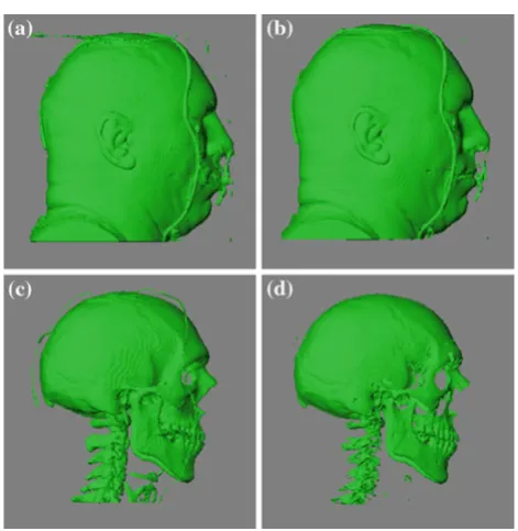
As each of the 8 vertex cells has only two possible states, there is a total of 28 = 256 cases of intersection between isosurface and cell edge, which are listed in a lookup-table. However, some pairs of these cases are symmetric or com-plementary to each other, which restrains the problem to 15 cases, as illustrated in Fig.1. A demonstration of the march-ing cubes algorithm usmarch-ing different isovalues is shown in Fig.2.
The pseudocode of the marching cubes technique can be briefly described according to the Algorithm 1. The advan-tage of this algorithm is that the processing of a cell is inde-pendent of the other ones, which allows its parallelization. However, as a disadvantage, it may generate holes in the iso-surfaces, due to topological ambiguities of the cases.
Algorithm 1 runs in timeO(n), wherenis the total num-ber of processed cells. On the other hand, many of these cells are empty, incurring an unnecessary waste of time. To minimize this waste, some spatial data structures are used to only process the active cells, that is, the ones that are
Fig. 2 Volume rendering of a male head dataset using marching cubes with different isovalues:a30,b50,c75,d100
intercepted by an isosurface, reducing the complexity of the algorithm.
In the context of the acceleration of marching cubes algo-rithm on the GPU, Johansson and Carr [18] conducted a com-parative analysis of its execution using data structures, such as k-d trees [2] and interval trees [5], reporting the rendering rate speedups obtained in relation to the CPU. Their approach is based on a caching cell topology technique, which stores the 15 cases of marching cubes in GPU (once it can cache geometry in a very efficient way) and improves the perfor-mance of the case classification stage by means of an opti-mization of the pre-computation step on the CPU, making use of the span-space properties. The method achieves a maxi-mum speedup (between the GPU acceleration with an inter-val tree and its CPU counterpart) of 4.3 times. However, the authors do not make experiments with larger datasets due to hardware limitations.
reconstruction, but their approach does not use any accel-erating data structures to improve the overall performance of the algorithm, obtaining a maximum speedup of approxi-mately 2.0 times.
Newman and Yi [32] developed an in-depth research about the possibilities of developing the marching cubes tech-nique, describing their respective properties, extensions and attempts to solve its limitations. However, the paper only shows the differences between these possibilities in terms of algorithm complexity as well as visualization results, and does not make an analysis with volume datasets.
Smistad et al. [43] presented an implementation of the marching cubes algorithm written in OpenCL [37] that runs entirely in the GPU. Like [6], it uses the idea of histogram pyramids to generate the output stream of vertices to be ren-dered and runs as fast as CUDA and shader implementations, providing a very efficient storage scheme as well. However, the drawback of their implementation lies on the interoper-ability between OpenCL and OpenGL.
Concerning recent applications that make use of the marching cubes algorithm in GPU, Dembogurski et al. [7] used a marching cubes histogram pyramid implementation for a procedural terrain generation; Donlon et al. [8] acceler-ated the visualization and quantification of MRI datasets to help in the treatment of patients that suffer from rheumatoid and psoriatic arthritis; Kim et al. [21] presented a method for computing the surfaces of a protein molecule in inter-active time; Lang et al. [23] developed an environment for fast and automated analysis of large SBFSEM (serial block-face scanning electron microscopy) datasets to extract neuron morphologies.
2.4 Accelerating data structures
There are several classes of data structures that are very useful to avoid the processing of empty cells. One of them consists of interval-based representations, which uses cell intervals to group cells [32]. The advantage of this type of representation is in its flexibility, being applied not only on regular grids, but also on non-regular grids, once it works from an interval space, instead of using the mesh space itself.
The main methods of this class are based on a represen-tation called span-space [28], where each cell of the volume data is mapped to a two-dimensional point, whose coordi-natesxandycorrespond, respectively, to the minimum and maximum values among the eight vertices that constitute a cell. From a given isovalueh, the points of the span-space that represent the active cells are the ones wherex ≤hand y≥h.
A general scheme of the span-space is shown in Fig.3. The blue area corresponds to the active cells of a volume data and the yellow areas to the cells that are not rendered, due to the fact thatx >h(yellow area located right of the blue
Fig. 3 Representation of the span-space proposed by Livnat et al. [28]
area) ory<h(yellow area located below the blue area). No cell can be mapped to the red area, once xis never greater thany.
This section describes some spatial data structures and how they can be used to improve the performance of the marching cubes algorithm.
2.4.1 k-d tree
The k-d tree [2] is a special case of the binary search tree, used to organize points located in a k-dimensional space. Each non-leaf node represents a splitting hyperplane that divides the space into two parts in a specific direction, which is defined according to the depth of this node in the tree. The left subtree contains all the points located at the left of the hyperplane and the right subtree contains the ones to the right. The leaf nodes store one point each.
In the marching cubes algorithm, the volume data is mapped onto a span-space before constructing the tree, once the queries in the k-d tree are faster when working with points in a 2D plane rather than in a 3D space. Furthermore, every node stores a point in the span-space, instead of storing the points only in the leaves. The construction takesO(nlogn) time, wherenis the total number of cells in the volume data, and demands a storage space ofO(n).
When searching in the tree, given an isovalue h, it will traverse only the nodes that correspond to the active cells of the volume data. Thus, the query takes O(√n+ p)time, where pis the number of active cells.
2.4.2 Interval tree
of the binary search tree, and allows an efficient search of all intervals that overlap with a given interval or point.
The root of the tree stores a value that corresponds to the median of the endpoints of all intervals and a list of intervals that contain this value. The left subtree stores the intervals that are completely below the median and the right subtree stores the ones completely above the median. Then, the process is repeated recursively for each subtree. It takes a construction time of O(nlogn)and, like the k-d tree, a storage space ofO(n).
The span-space is suitable for constructing an interval tree. In this case, the intervals correspond to the volume cells, and the endpoints are the minimum and maximum values of the cell, which stands for its coordinates in the span-space.
Searching in an interval tree takes O(logn + p)time, where pis the number of active cells, which makes it more efficient than the k-d tree. On the other hand, it demands higher memory space.
2.4.3 Quadtree and octree
A quadtree [12] is a tree data structure where every non-leaf node has exactly four children. It is used to partition a region in a 2D space into four equal regions (or quadrants). These regions are then partitioned into other four subregions, and so on, until the subregion is empty, which characterizes a leaf node. The 3D analogous structure of a quadtree is called octree, which partitions a 3D space region into eight subregions (or octants).
Once the span-space is a 2D space, it can be represented by a quadtree. Letlbe the number of bits used to store the volume data values, which means that there are 2l possible values (ranging between 0 and 2l−1) for a vertex cell. Thus, the span-space is a 2l×2lregion, and the points correspond to the mapped cells. Every node in the tree stores the information of a point in the span-space.
However, more than one cell can be mapped to a same point in the span-space. To overcome this problem, each node in the quadtree also stores a pointer to a list of the volume data cells that were mapped to this point. Then, the queries can be made as usual, traversing the nodes corresponding to the active cells.
In the octree case, the tree is built directly from the volume data. However, in case of non-regular grids (i.e., when vol-ume dimension is not a power of two), the subregions have different sizes, once we are partitioning cell regions.
3 Methodology
The significant evolution of the programmability of the graphics hardware has allowed the isosurface extraction pro-cedure to be accelerated by the GPU, taking advantage of
its parallel architecture. However, the bus used to establish a communication between the CPU and the GPU is a bot-tleneck for this acceleration, which means that transferring all the tasks to the GPU may not be the best solution. Thus, in order to maximize the performance of this procedure, an adequate planning of the graphics pipeline is needed, picking up the tasks that can be run on the CPU and the ones that can be transferred to the GPU, as well as a proper use of all the memory hierarchy. Some proposals of graphics pipeline for isosurface extraction were made by Buatois et al. [3], Johans-son [17], Martin et al. [31], Pascucci [38], Reck et al. [40], and Tatarchuk et al. [44].
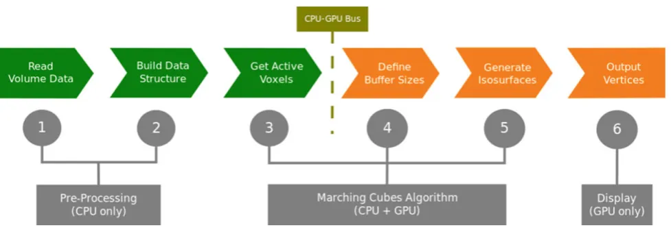
The methodology proposed in this work is restricted to the marching cubes technique, rather than generalizing to the isosurface extraction process. Figure4shows a general scheme, composed of six stages. At the Stage 1, the CPU reads a volume dataset of dimensionsNx×Ny×Nz, which
is then allocated both in the main memory (RAM, used by the CPU) and in the video memory (VRAM, used by the GPU). Except for the octree, an extra memory space is allocated for the span-space related to the volume data.
Later, one of the spatial data structures described in Sect.2.4is constructed from the volume data and stored only in the main memory (stage 2). Then, the volume data is freed from the main memory, but it remains allocated in the video memory.
Algorithm 2 details the two aforementioned stages of the scheme. Once the preprocessing stage is done, the march-ing cubes algorithm is started (stage 3). From an isovalueh specified by the user, the CPU performs a search in the data structure, traversing only the nodes that correspond to the active volume cells, and creating a list of these cells, which is then transferred to the GPU via communication bus.
Fig. 4 Our method for acceleration of the marching cubes algorithm. Stages 1 and 2 are responsible for the preprocessing stage; stages 3 to 5 correspond to the execution of marching cubes and stage 6 makes
the display of vertices on the screen.Green boxesstand for the actions executed on CPU, whereas the orange boxes the ones on GPU
in the cell. After this procedure is done for all active cells, the total number of vertices to be output can be determined, which will define the exact size of video memory needed to allocate two vertex buffers: one for storing these vertices and other for their respective normals (stage 4).
After that, the list of active cells is traversed by the GPU once more to generate the triangles that comprise the iso-surfaces (stage 5). For each active cell of the list, the GPU calculates the isosurface intersections with the 12 edges of the cell by interpolating the vertices and the normals calcu-lated by the GPU from the volume data. Once the cell index and the intersections are found, the GPU obtains the list of vertices and normals related to the isosurface, writing them in the respective vertex buffers. Finally, the volume data is rendered from these buffers (stage 6).
All the procedures executed by the GPU are parallelized, once the results obtained from a cell are independent of the others. However, the speedup achieved with the acceleration of the marching cubes relies on the way this parallelization occurs. When a task is assigned to the GPU, it creates a specific amount of blocks.1 All of these blocks contain a specific number of threads (which is the same for all blocks), responsible for running a part of this task.
The amount of blocks to be created depends on the number of active cells and the number of threads per block, also known as block size. The block size is chosen in such a way that it is neither too low, assigning much work for all threads and not maximizing the task performance at all, nor too high, causing an overhead of starting and terminating threads.
The parallel processing of the list of active cells is made from a specific program, called GPU kernel. In our work, the GPU kernel was implemented using the CUDA architecture.
1Concept from CUDA programming model [35].
In addition to the algorithms that are responsible for the exe-cution of the marching cubes technique, some of the GPU inherent resources were employed in order to improve the rendering rate of the volume data. Among these resources are the use of texture memory, which is faster for handling read-only data, to store the lookup-tables employed by the marching cubes algorithm and the volume data itself, and the use of shared memory, which permits the data sharing among threads contained in a same block, besides being faster than the standard video memory. In the GPU marching cubes algo-rithm, the shared memory is used to compute, for each active cell, the intersections between an isosurface contained in the cell and the cell edges.
The pseudocodes of the following algorithms were adapted from [36]. Before the execution of these algorithms, the respective number of blocks (as well as their sizes) used to help on the parallelization of their procedures are deter-mined.
Algorithm 3 represents the first step of the execution of marching cubes in GPU (stage 4 of Fig.4). The goal of this algorithm is to calculate the exact amount of video memory that will be used to store the vertices and the normals related to the volume data. Once this amount is obtained, the GPU allocates the appropriate space in the vertex buffers, which will then store the vertices to be output and their respective normals.
4 Experimental results
The tests were executed on an AMD Phenom II X6 1090T 3.2 GHz processor with 8 GB of RAM, and an NVIDIA GeForce GTS 450 with 1 GB of VRAM (together with its most recent drivers), using a C-like programming language, OpenGL 4.2 and CUDA 4.1 APIs.
The experiments were made using 8-bit datasets from [1] and [45], where each scalar value ranges from 0 to 255. Table
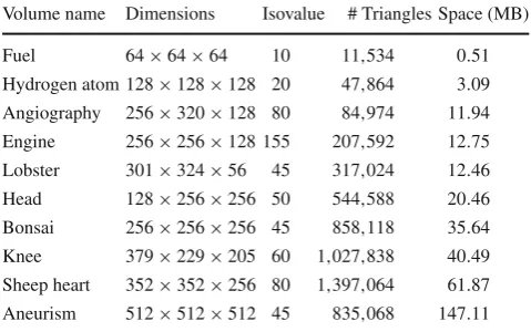
Table 1 List of volume datasets with their respective sizes in voxels, isovalues, number of triangles and memory space allocated during exe-cution of marching cubes algorithm (in megabytes)
Volume name Dimensions Isovalue # Triangles Space (MB) Fuel 64×64×64 10 11,534 0.51 Hydrogen atom 128×128×128 20 47,864 3.09 Angiography 256×320×128 80 84,974 11.94 Engine 256×256×128 155 207,592 12.75 Lobster 301×324×56 45 317,024 12.46 Head 128×256×256 50 544,588 20.46 Bonsai 256×256×256 45 858,118 35.64 Knee 379×229×205 60 1,027,838 40.49 Sheep heart 352×352×256 80 1,397,064 61.87 Aneurism 512×512×512 45 835,068 147.11
1shows a list of volume datasets used in the tests, together with their respective dimensions (in voxels), isovalues (input to the marching cubes algorithm), number of triangles ren-dered in the screen (which depends on the isovalue), and memory space allocated during the execution of the march-ing cubes algorithm, which corresponds to the size of the volume datasets (1 byte per voxel) plus the amount of the vertex and normal buffers (4 bytes per vertex and normal, which leads to a total of 24 bytes per triangle, once there are two buffers). The isovalues for “Fuel”, “Hydrogen atom” and “Engine” datasets were the same as those used by [18], so that a more accurate comparison can be made. The results of the rendering of each dataset, made from the application described in this work, are shown in Fig.5.
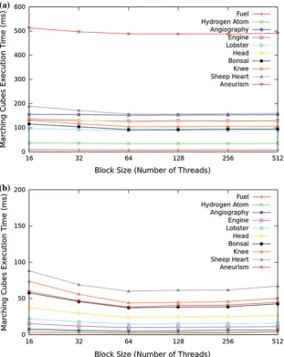
Figure6shows two plots that illustrate the average time (in milliseconds) of 50 executions of the marching cubes imple-mentation on the GPU for different block size values, using each of the volume datasets and their respective isovalues listed in Table1. The plot (a) stands for the executions of a brute force implementation of the marching cubes algorithm that runs without the aid of accelerating data structures and sequentially traverses all voxels of a volume dataset (includ-ing the empty ones), and (b) the executions us(includ-ing an interval tree to store the voxels from the datasets. From both plots, it can be noticed that for block sizes of 64 and higher, the run-ning time of the marching cubes increases very slightly, and it does not rely on whether a data structure is used or not for acceleration. In other words, for any data structure used in the marching cubes algorithm, the behavior of the curves in the plot will be the same. As mentioned in Sect.3, although a higher number of threads means higher parallelization, the time spent to create the threads also gets higher, hence sta-bilizing the performance. Thus, all the tests were run with a block size value of 64.
Table2shows the average frame rate of the execution of marching cubes algorithm in CPU and GPU, for all data struc-tures described in Sect.2.4, and comparing to their respective CPU versions of the algorithm. These results do not consider the time spent on the pre-processing stages (volume data reading and data structure construction), regarding only the events that occur between the search in the data structure and the volume display on the screen (Stages 3–6 of Fig.4).
Fig. 5 Rendering results of each dataset generated by the application, with the isovalues listed in Table1.aFuel,bhydrogen atom,cangiography, dengine,elobster,fhead,gbonsai,hknee,isheep heart,janeurism
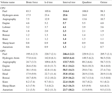
Table 2 Average frame rate (in frames per second) of the execution of marching cubes algorithm in CPU and GPU, with different data structures, comparing against the brute force version
Values betweenparenthesis
correspond to the acceleration factor related to their respective data structure versions of marching cubes in CPU for each volume dataset
Volume name Brute force k-d tree Interval tree Quadtree Octree CPU
Fuel 83.3 105.6 114.4 108.0 98.3
Hydrogen atom 17.5 23.4 25.6 24.0 19.2
Angiography 7.5 12.9 14.1 13.6 10.7
Engine 4.6 5.2 5.7 5.5 4.8
Lobster 3.2 3.7 4.1 3.9 3.6
Head 1.8 2.0 2.3 2.1 1.9
Bonsai 1.2 1.3 1.6 1.4 1.3
Knee 1.1 1.2 1.4 1.3 1.1
Sheep heart 0.8 0.9 1.0 0.9 0.8
Aneurism 0.6 0.9 1.3 1.2 0.7
GPU
Fuel 195.4 (2.3) 220.7 (2.1) 246.4 (2.2) 229.9 (2.1) 205.7 (2.1) Hydrogen Atom 77.0 (4.4) 142.8 (6.1) 165.0 (6.4) 149.5 (6.2) 96.5 (5.0) Angiography 24.7 (3.3) 109.6 (8.5) 133.7 (9.5) 89.2 (6.6) 58.7 (5.5) Engine 26.6 (5.8) 61.0 (11.7) 81.1 (14.2) 56.8 (10.3) 38.4 (8.0) Lobster 30.1 (9.4) 42.8 (11.6) 58.5 (14.3) 29.8 (7.6) 27.4 (7.6) Head 17.9 (9.9) 22.7 (11.4) 35.8 (15.6) 28.9 (13.8) 20.9 (11.0) Bonsai 10.7 (8.9) 13.2 (10.2) 25.9 (16.2) 18.7 (13.4) 11.5 (8.8) Knee 8.2 (7.4) 9.7 (8.1) 22.4 (16.0) 10.7 (8.2) 9.1 (8.2) Sheep Heart 6.3 (7.9) 7.4 (8.2) 16.3 (16.3) 8.9 (9.9) 6.6 (8.3) Aneurism 2.1 (3.5) 10.2 (11.3) 23.7 (18.2) 11.9 (9.9) 9.5 (13.5)
while the method proposed in this paper calculates them on-the-fly.
Another important fact to be pointed out is the perfor-mance of quadtree, which obtained a better frame rate than the k-d tree and the octree, standing only behind the interval tree. It achieved a maximum speedup of 13.8 times for the “Head” dataset. For the other datasets, excluding the “Fuel”, the speedup was between 6.2 and 10.3.
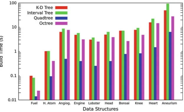
Concerning the building time of the data structures, quadtree had a much higher performance than the other ones, as shown in Fig.7. For all datasets used in the tests, the build-ing time of the quadtree was very much smaller than the other data structures, not having a significant gain of time as the volume datasets get larger, which is very efficient for real applications that process great amounts of volume data. For the rest of the data structures, the building time increases considerably among the datasets.
Octree provided the second best building times. Even though its building algorithm is similar to the one of quadtree, the fact that it is applied in the 3D space brings on a higher waste of time, once the total number of subdivisions is higher. In third place, comes the k-d tree, which has a worse build-ing time than the octree because of the successive executions of the algorithm that finds the median of the points located in the span-space. Finally, interval tree achieved the worst
building times among the tested data structures. It happened due to the time spent in sorting the cell lists, which has a higher time complexity than finding a median.
The bottleneck of this approach resides on the fact that the searches in the data structures are done on the CPU. It is feasible to implement all of the data structure algorithms on the GPU, as well as storing the data structure itself in the video memory, but since most of the tree search algorithms are recursive and CUDA does not support recursions, if non-recursive versions of these algorithms were implemented on the GPU, there would have a large waste of time and space to create stacks and loops used to simulate the eventual recursive calls.
5 Conclusions and future work
Fig. 7 Average building times of the data structures for each volume dataset
This paper described a comparative analysis among four different spatial data structures for speeding up the marching cubes algorithm through graphics processing units, together with an approach using CUDA framework. Time complexity of the algorithm depends on the volume data cells that contain an isosurface, instead of the total number of cells, avoiding the processing of empty cells.
Experimental results obtained from several volumetric datasets demonstrate that it was possible to accelerate the marching cubes algorithm by a factor of approximately 18 times when compared to the CPU approach.
Among the four data structures described in this paper, interval tree provided the best rendering rates, but the time spent in building the structure was relatively high. On the other hand, quadtree achieved very satisfactory building times, even for large volume datasets, besides slightly lower rendering rates compared to those of the acceleration with an interval tree. However, since the building of a data struc-ture is done only once, while the search is performed when-ever the volume needs to be rendered, it is more worth-while to use the interval tree rather than the quadtree in this case.
Directions for future work include the implementation of the data structures mentioned in this paper on the GPU, together with their respective building and searching oper-ations so that they can be done in parallel, and an exten-sion of the proposed method to open frameworks, such as OpenCL [37], once that CUDA framework is restricted to NVIDIA [35] graphic cards. Furthermore, a case study with more powerful graphic cards (such as those from NVIDIA Kepler architecture) is desired as well.
Acknowledgments The authors are grateful to FAPESP, CNPq, and National Institute of Science and Technology in Medicine Assisted by Scientific Computing (INCT/MACC) for the financial support.
References
1. The volume library.http://lgdv.cs.fau.de/External/vollib
2. Bentley J (1975) Multidimensional binary search trees used for associative searching. Commun ACM 18(9):509–517
3. Buatois L, Caumon G, Lévy B (2006) GPU accelerated isosurface extraction on tetrahedral grids. In: Advances in visual comput-ing. Lecture notes in computer science, vol 4291, Springer, Berlin, pp 383–392
4. Chan S, Purisima E (1998) A new tetrahedral tesselation scheme for isosurface generation. Comput Graph 22(1):83–90
5. Cignoni P, Marino P, Montani C, Scopigno R (1997) Speeding up isosurface extraction using interval trees. IEEE Trans Visual Comput Graph 3:158–170
6. Ciznicki M, Kierzynka M, Kurowski K, Ludwiczak B, Napierala K, Palczynski J (2011) Efficient isosurface extraction using marching tetrahedra and histogram pyramids on multiple GPUs. In: Proceed-ings of the 9th international conference on parallel processing and applied mathematics, Torun, Poland, pp 343–352
7. Dembogurski B, Clua E, Vieira M, Leta F (2008) Procedural terrain generation at GPU level with marching cubes. In: Proceedings of the VII Brazilian symposium of games and digital entertainment— computing track, Belo Horizonte, MG, Brazil, pp 37–40 8. Donlon B, Veale D, Brennan P, Gibney R, Carr H, Rainford L,
Ng C, Pontifex E, McNulty J, FitzGerald O, Ryan J (2012) MRI-based visualisation and quantification of rheumatoid and psoriatic arthritis of the knee. In: Visualization in medicine and life sciences II, mathematics and visualization, Springer, pp 45–59
9. Dürst M (1988) Letters: additional reference to marching cubes. ACM Comput Graph 22(4):72–73
10. Dyken C, Ziegler G, Theobalt C, Seidel H (2008) High-speed marching cubes using histopyramids. Comput Graph 27(8):2028– 2039
11. Elvins T (1992) A survey of algorithms for volume visualization. SIGGRAPH Comput Graph 26(3):194–201
12. Finkel R, Bentley J (1974) Quad trees: a data structure for retrieval on composite keys. Acta Inf 4(1):1–9
13. Goetz F, Junklewitz T, Domik G (2005) Real-time marching cubes on the vertex shader. In: Eurographics. Dublin, Ireland
15. Guéziec A, Hummel R (1995) Exploiting triangulated surface extraction using tetrahedral decomposition. IEEE Trans Visual Comput Graph 1(4):328–342
16. Jeffreys H, Jeffreys B (1988) Central differences formula. In: Meth-ods of mathematical physics, Cambridge University Press, Cam-bridge, pp 284–286
17. Johansson G (2005) Accelerating isosurface extraction by caching cell topology with graphics hardware. Master’s thesis, University College Dublin, Ireland
18. Johansson G, Carr H (2006) Accelerating marching cubes with graphics hardware. In: Proceedings of the conference of the cen-ter for advanced studies on collaborative research. Toronto, ON, Canada
19. Kaufman A (1991) Volume visualization. IEEE Computer Society Press, Los Alamitos
20. Keppel E (1975) Approximating complex surfaces by triangulation of contour lines. IBM J Res Dev 19(1):2–11
21. Kim B, Kim K, Seong J (2012) GPU accelerated molecular surface computing. Appl Math Inf Sci 6(1S):185S–194S
22. Lacroute P (1996) Fast volume rendering using a shear-warp fac-torization of the viewing transformation. PhD thesis, Stanford Uni-versity, Stanford, CA, USA
23. Lang S, Drouvelis P, Tafaj E, Bastian P, Sakmann B (2011) Fast extraction of neuron morphologies from large-scale SBFSEM image stacks. J Comput Neurosci 31(3):533–545
24. Lengyel E (2010) Transition cells for dynamic multiresolution marching cubes. J Graph GPU Game Tools 15(2):99–122 25. Levoy M (1990) Efficient ray tracing of volume data. ACM Trans
Graph 9(3):245–261
26. Li T, Xie M, Zhao W, Wei Y (2010) Shear-warp rendering algo-rithm based on radial basis functions interpolation. In: Proceedings of the 2nd international conference on computer modeling and sim-ulation, Sanya, China, pp 425–429
27. Liu B, Clapworthy G, Dong F (2009) Accelerating volume raycast-ing usraycast-ing proxy spheres. Comput Graph Forum 28(3):839–846 28. Livnat Y, Shen HW, Johnson R (1996) A near optimal isosurface
extraction algorithm using the span space. IEEE Trans Visual Com-put Graph 2(1):73–84
29. Lorensen W, Cline H (1987) Marching cubes: a high resolution 3D surface construction algorithm. Comput Graph 21(4):163–169 30. Lum EB, Wilson B, liu Ma K (2004) High-quality lighting and
efficient pre-integration for volume rendering. In: Proceedings of the joint Eurographics—IEEE TVCG symposium on visualization, pp 25–34
31. Martin S, Shen HW, McCormick P (2010) Load-balanced isosur-facing on multi-GPU clusters. In: Proceedings of the Eurograph-ics symposium on parallel graphEurograph-ics and visualization, Norrküping, Sweden, pp 91–100
32. Newman T, Yi H (2006) A survey of the marching cubes algorithm. Comput Graph 30(5):854–879
33. Nielson GM, Hamann B (1991) The asymptotic decider: resolv-ing the ambiguity in marchresolv-ing cubes. In: Proceedresolv-ings of the 2nd conference on visualization, San Diego, CA, USA, pp 83–91
34. Nurzy´nska K (2009) 3D object reconstruction from parallel cross-sections. In: Bolc L, Kulikowski J, Wojciechowski K (eds) Com-puter vision and graphics. Lecture notes in comCom-puter science, vol 5337, Springer, Berlin, pp 111–122
35. NVIDIA CUDA C programming guide version 3.2. http:// developer.download.nvidia.com/compute/cuda/3_2_prod/toolkit/ docs/CUDA_C_Programming_Guide.pdf
36. NVIDIA (2012) CUDA C/C++ SDK code examples. http:// developer.nvidia.com/cuda-cc-sdk-code-samples
37. OpenCL The khronos group.http://www.khronos.org/opencl/
38. Pascucci V (2004) Isosurface computation made simple: hardware acceleration, adaptive refinement and tetrahedral stripping. In: Pro-ceedings of the joint Eurographics—IEEE TVCG symposium on visualization, Konstanz, Germany, pp 293–300
39. Pöthkow K, Weber B, Hege HC (2011) Probabilistic marching cubes. Comput Graph Forum 30(3):931–940
40. Reck F, Dachsbacher C, Grosso R, Greiner G, Stamminger M (2004) Realtime isosurface extraction with graphics hardware. In: Proceedings of the Eurographics 2004 short presentations and inter-active demos, Grenoble, France, pp 33–36
41. Schindler B, Fuchs R, Waser J, Peikert R (2011) Marching correctors—fast and precise polygonal isosurfaces of SPH data. In: Proceedings of the 6th international smoothed particle hydrody-namics European research interest community (SPHERIC) work-shop, Hamburg, Germany, pp 125–132
42. Schlegel P, Pajarola R (2009) Layered volume splatting. In: Advances in visual computing, lecture notes in computer science, vol 5876, Springer, pp 1–12
43. Smistad E, Elster AC, Lindseth F (2011) Fast surface extraction and visualization of medical images using openCL and GPUs. In: Proceedings of the joint workshop on high performance and dis-tributed computing for medical imaging, Toronto, Canada 44. Tatarchuk N, Shopf J, DeCoro C (2007) Real-time isosurface
extraction using the GPU programmable geometry pipeline. In: Proceedings of the ACM SIGGRAPH 2007 courses, San Diego, CA, USA, pp 122–137
45. Volvis: volume datasets.http://www.volvis.org
46. Wang Z, Fan B, Li N, Zhang H (2009) Iso-surface extraction and optimization method based on marching cubes. In: Proceedings of the international conference on semantics, knowledge and grid, Zhuhai, China, pp 458–460
47. Westover L (1990) Footprint evaluation for volume rendering. In: Proceedings of the 17th annual conference on computer graphics and interactive techniques, Dallas, TX, USA, pp 367–376 48. Wilhelms J (1990) A coherent projection approach for direct
vol-ume rendering. Technical report of University of California, Santa Cruz, CA, USA
![Fig. 3 Representation of the span-space proposed by Livnat et al. [28]](https://thumb-us.123doks.com/thumbv2/123dok_us/862987.1583800/4.595.308.542.55.250/fig-representation-span-space-proposed-livnat-et-al.webp)