O R I G I N A L A R T I C L E
Open Access
Deep-learning-based motion-correction
algorithm in optical resolution
photoacoustic microscopy
Xingxing Chen
1, Weizhi Qi
2and Lei Xi
2*Abstract
In this study, we propose a deep-learning-based method to correct motion artifacts in optical resolution
photoacoustic microscopy (OR-PAM). The method is a convolutional neural network that establishes an end-to-end map from input raw data with motion artifacts to output corrected images. First, we performed simulation studies to evaluate the feasibility and effectiveness of the proposed method. Second, we employed this method to process images of rat brain vessels with multiple motion artifacts to evaluate its performance for in vivo applications. The results demonstrate that this method works well for both large blood vessels and capillary networks. In comparison with traditional methods, the proposed method in this study can be easily modified to satisfy different scenarios of motion corrections in OR-PAM by revising the training sets.
Keywords:Deep learning, Optical resolution photoacoustic microscopy, Motion correction
Introduction
Optical resolution photoacoustic microscopy (OR-PAM) is a unique sub-category of photoacoustic imaging (PAI) [1–3]. Via the combination of sharp-focused pulsed laser and high-sensitivity detection of rapid thermal expansion-induced ultrasonic signals, OR-PAM offers both an optical-diffraction limited lateral resolution of micrometers and an imaging depth of millimeters. With these special features, OR-PAM is extensively employed in the studies of biology, medicine, and nanotechnology [4]. However, high-resolution imaging modalities are also extremely sensitive to motion artifacts, which are primarily attributed to the breath and heartbeat of animals. Motion artifacts are nearly inevitable for imaging in vivo targets, which cause a loss of key information for the quantitative analysis of images. Therefore, the exploration of image-processing methods that can reduce the influence of motion artifacts in OR-PAM is necessary.
Recently, several motion-correction methods have been proposed for PAI to obtain high-quality images [5–8]. The majority of existing algorithms are primarily based on deblurring methods that are extensively employed in
photoacoustic-computed tomography (PACT) and only suitable for cross-sectional B-scan images [5, 6]. Schwarz et al. [7] proposed an algorithm to correct motion artifacts between adjacent B-scan images for acoustic-resolution photoacoustic microscopy (AR-PAM). Unfortunately, the algorithm needs a dynamic reference, which is not feasible in high-resolution OR-PAM images. A method presented by Zhao et al. [8] has the capability of addressing these shortcomings but can only correct the dislocations along the direction of a slow-scanning axis. Recent methods that are based on deep learning have demonstrated a state-of-the-art performance in many fields, such as natural lan-guage processing, audio recognition and visual recognition [9–14]. Deep learning discovers an intricate structure by using a backpropagation algorithm to indicate how a net should change its internal parameters, which are used to compute the representation in each layer from that in the previous layer. A convolutional neural network (CNN) is a common model for deep learning in image processing [15]. In this study, we present a fully CNN [16] to correct mo-tion artifacts in a maximum amplitude projecmo-tion (MAP) image of OR-PAM instead of a volume. To evaluate the performance of this method, we conduct both simulation tests and in vivo experiments. The experimental results
© The Author(s). 2019Open AccessThis article is distributed under the terms of the Creative Commons Attribution 4.0 International License (http://creativecommons.org/licenses/by/4.0/), which permits unrestricted use, distribution, and reproduction in any medium, provided you give appropriate credit to the original author(s) and the source, provide a link to the Creative Commons license, and indicate if changes were made.
* Correspondence:[email protected]
2Department of Biomedical Engineering, Southern University of Science and
Technology, Shenzhen 518055, Guangdong, China
Full list of author information is available at the end of the article
Visual Computing for Industry,
Biomedicine, and Art
indicated that the presented method can eliminate displace-ments in both simulations and in vivo MAP images.
Methods
Experimental setup
The OR-PAM system in this study has been described in previous publications [17]. A high-repetition-rate laser serves as an irradiation source with a repetition rate of 50 KHz. A laser beam is coupled into a single mode fiber, collimated via a fiber collimation lens (F240FC-532, Thorlabs Inc.), and focused by an object-ive lens to illuminate a sample. A customized micro-electro-mechanical system scanner is driven by a multi-functional data acquisition card (PCI-6733, National In-strument Inc.) to realize fast raster scanning. We detect photoacoustic signals using a flat ultrasonic transducer with a center frequency of 10 MHz and a bandwidth of 80% (XMS-310-B, Olympus NDT). The original photo-acoustic signals are amplified by a homemade pre-amplifier at ~ 64 dB and digitized by a high-speed data acquisition card at a sampling rate of 250 MS/s (ATS-9325, Alazar Inc.). The imaging reconstruction is per-formed using Matlab (2014a, MathWorks). We derived
the envelopes of each depth-resolved photoacoustic sig-nal using the Hilbert transform and projected the max-imum amplitude along the axial direction to form a MAP image. We implemented our algorithm for mo-tion correcmo-tion using a tensor flow package and trained this neural network using Python software on a per-sonal computer.
Algorithm of CNN
Figure 1 illustrates an example of the mapping pro-cesses of CNN. In this case, the input is a two-dimensional 4 × 4 matrix, and the convolution kernel is a 2 × 2 matrix. First, we select four adjacent ele-ments (a, b, e, f) in the upper right corner of the
in-put matrix, multiply each element with the
corresponding element in the convolution kernel, and sum all calculated elements to form S1 in the output matrix. We repeat the same procedure by shifting the 4 × 4 matrix by one pixel in either direc-tion of the input matrix to calculate the remaining pixel values in the output matrix. The CNN is classi-fied by two major properties: local connectivity and param-eter sharing. As depicted in Fig. 1, the element S1 is not
Fig. 1Mapping processes of convolutional neural network
associated with all elements in the input layer; it is only asso-ciated with a small number of elements in a spatially local-ized region (a, b, e, f). A hidden layer has several feature maps, and all hidden elements within a feature map share the same parameter, which further reduces the number of parameters.
The structure of the CNN in this work is illustrated in Fig. 2. The images with the motion artifacts used for training were obtained from the ground-truth image. As depicted in Fig.2, the method consists of three convolu-tional layers. The first convoluconvolu-tional layer can be expressed as
G1¼Relu W1ð IþB1Þ ð1Þ
where the rectified linear unit (Relu) is a nonlinear func-tion max(0, z) [18], W1 is the convolution nucleus, ∗ de-notes the convolution operation, I is the original image, and B1 is the neuron bias vector. The second convolutional layer, which is a nonlinear mapping, can be defined as
G2¼Relu W2ð G1þB2Þ ð2Þ
where Relu, W2, B2, and∗are defined according to the previously defined expression. In comparison with the
Fig. 3Results of simulation experiment
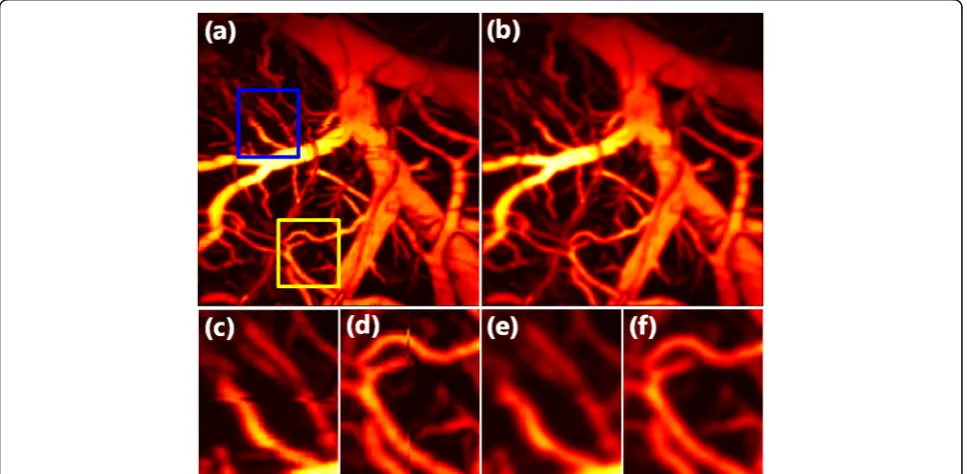
Fig. 4Results of correcting motion artifacts in horizontal and vertical dislocation.aMAP image that corresponds to the raw data of a rat brain.b
MAP image after motion correction.canddEnlarged images of the two boxes in (a).eandfEnlarged figures of corresponding areas in (b)
first two layers, a nonlinear function does not exist in the last layer, which is used to reconstruct the output image. The last layer can be defined as follows:
O¼ðW3G2þB3Þ ð3Þ
Similarly, W3and B3are defined according to the pre-viously defined expression. In this study, the input and output images have one channel; thus, the size of the convolution nucleus W1, W2, and W3are set to [5, 5, 1, 64], [5, 5, 64, 64], and [5, 5, 64, 1], respectively. The size of the neuron bias vectors B1, B2, and B3are set to [64], [64], and [1], respectively.
Training
Learning the end-to-end mapping function M requires estimation of the network parameters Φ = { W1, W2, W3, B1, B2, B3 }. The purpose of the training process is to estimate and optimize the parameters W1, W2, W3, B1, B2, and B3, which is achieved by minimizing the error
between the reconstructed images M(O;Φ) and the cor-responding input images I. Given a set of motion images and their corresponding non-motion images, we use the mean squared error as the loss function:
Lð Þ ¼Φ n1Xni¼1kM Oð i;ΦÞ−Iik2 ð4Þ
where nis the number of training samples. The error is minimized using the gradient descent with standard backpropagation [19]. To avoid changing the image size, all convolutional layers are set to the same padding.
Results
After the training, we conducted a series of experi-ments to evaluate the performance of the method. In the simulation, we created a displacement along the direc-tion of the Y axis, which is denoted by a white arrow (Fig. 3(a)). We processed the image with the trained CNN and obtained the results, as depicted in Fig. 3(b). In comparison with the images before and after the
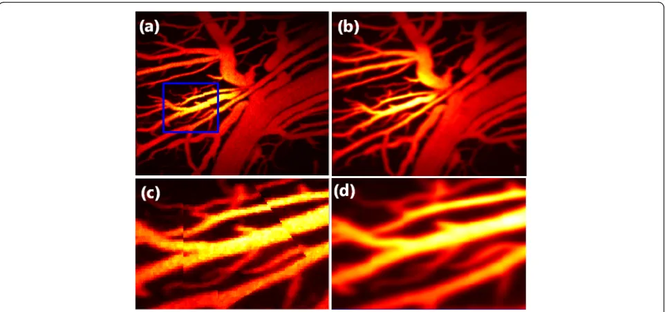
Fig. 5Results of correcting motion artifacts in an arbitrary dislocation.aMaximum amplitude projection (MAP) image that corresponds to the raw data of a rat brain.bMAP image after motion correction.cEnlarged image of the box in (a).dEnlarged figure of corresponding areas in (b)
processing, we observe that the displacement has been corrected, which demonstrates that our algorithm works well in simulation cases.
We created both horizontal artifacts and vertical mo-tion artifacts, as depicted in Fig.4(a). Figure4(c) and (d) illustrate an enlarged view of the motion artifacts in the blue rectangle and yellow rectangle, respectively. Figure 4(b) depicts the corrected MAP image via the proposed method, in which both the horizontal artifact and the vertical motion artifact have been corrected, as depicted in Fig.4(e) and Fig.4(f).
To demonstrate that our method can adequately cor-rect motion artifacts in an arbitrary dicor-rection, we estab-lished two complicated motion artifacts, as depicted in Fig. 5(a) and (c). Figure 5(b) and (d) illustrate the cor-rected MAP images, in which both displacements in the vertical and tilted directions have been corrected.
We evaluated the network performance using different kernel sizes. We conduct three experiments: (1) the ker-nel size in the first experiment has a size of 3 × 3; (2) the kernel size in the second one has a size of 4 × 4; and (3) the kernel size in the third experiment has a size of 5 × 5. The results in Fig.6 suggest that the performance of this algorithm can be significantly improved by using a larger kernel size. However, the processing efficiency will decrease. Thus, the choice of the network scale should always be a trade-off between performance and speed.
Conclusions
We experimentally demonstrated the feasibility of the pro-posed method using a CNN to correct motion artifacts in OR-PAM. In comparison with the existing algorithms [5–8], the proposed method demonstrates a better performance in eliminating motion artifacts in all directions without any ref-erence objects. Additionally, we verified that the perform-ance of the method improves as the kernel size increases. Although this method is designed for OR-PAM, it is capable of correcting motion artifacts in other imaging modalities, such as photoacoustic tomography, AR-PAM, and optical coherence tomography, when the corresponding training sets are used.
Abbreviations
AR-PAM:Acoustic-resolution photoacoustic microscopy; CNN: Convolutional neural network; MAP: Maximum amplitude projection; OR-PAM: Optical-resolution photoacoustic microscopy; PAI: Photoacoustic imaging
Acknowledgements
Not applicable
Authors’contributions
All authors read and approved the final manuscript.
Funding
This work was sponsored by National Natural Science Foundation of China, Nos. 81571722, 61775028 and 61528401.
Availability of data and materials
The datasets generated and/or analyzed during the current study are not publicly available due to personal privacy but are available from the corresponding author on reasonable request.
Competing interests
The authors declare that they have no competing interests.
Author details 1
School of Electronic Science and Engineering, University of Electronic Science and Technology of China, Chengdu 610054, Sichuan, China.
2
Department of Biomedical Engineering, Southern University of Science and Technology, Shenzhen 518055, Guangdong, China.
Received: 22 June 2019 Accepted: 23 September 2019
References
1. Wang LV, Yao JJ (2016) A practical guide to photoacoustic tomography in the life sciences. Nat Methods 13(8):627–638.https://doi.org/10.1038/nmeth.3925 2. Zhang HF, Maslov K, Stoica G, Wang LV (2006) Functional photoacoustic
microscopy for high-resolution and noninvasive in vivo imaging. Nat Biotechnol 24(7):848–851.https://doi.org/10.1038/nbt1220
3. Wang LV, Hu S (2012) Photoacoustic tomography: in vivo imaging from organelles to organs. Science 335(6075):1458–1462.https://doi.org/10.1126/ science.1216210
4. Beard P (2011) Biomedical photoacoustic imaging. Interface Focus 1(4): 602–631.https://doi.org/10.1098/rsfs.2011.0028
5. Taruttis A, Claussen J, Razansky D, Ntziachristos V (2012) Motion clustering for deblurring multispectral optoacoustic tomography images of the mouse heart. J Biomed Opt 17(1):016009.https://doi.org/10.1117/1.JBO.17.1.016009 6. Xia J, Chen WY, Maslov KI, Anastasio MA, Wang LV (2014) Retrospective
respiration-gated whole-body photoacoustic computed tomography of mice. J Biomed Opt 19(1):016003.https://doi.org/10.1117/1.JBO.19.1.016003 7. Schwarz M, Garzorz-Stark N, Eyerich K, Aguirre J, Ntziachristos V (2017)
Motion correction in optoacoustic mesoscopy. Sci Rep 7(1):10386.https:// doi.org/10.1038/s41598-017-11277-y
8. Zhao HX, Chen NB, Li T, Zhang JH, Lin RQ, Gong XJ et al (2019) Motion correction in optical resolution photoacoustic microscopy. IEEE Trans Med Imaging 38(9):2139–2150.https://doi.org/10.1109/TMI.2019.2893021 9. LeCun Y, Bengio Y, Hinton G (2015) Deep learning. Nature 521(7553):
436–444.https://doi.org/10.1038/nature14539
10. Mohamed AR, Dahl G, Hinton G (2009) Deep belief networks for phone recognition. In Proc. of NIPS workshop on deep learning for speech recognition and related applications, December, Whistler
11. Dahl GE, Ranzato M, Mohamed AR, Hinton G (2010) Phone recognition with the mean-covariance restricted Boltzmann machine. In: abstracts of the 23rd international conference on neural information processing systems, ACM, Vancouver, British Columbia, Canada, 6-9 December 2010
12. Rifai S, Dauphin YN, Vincent P, Bengio Y, Muller X (2011) The manifold tangent classifier. In: abstracts of the 24th international conference on neural information processing systems, ACM, Granada, Spain, 12-15 December 2011
13. Jarrett K, Kavukcuoglu K, Ranzato M, LeCun Y (2009) what is the best multi-stage architecture for object recognition? In: abstracts of the 2009 IEEE 12th international conference on computer vision, IEEE, Kyoto, Japan, 29 September-2 October 2009 DOI:https://doi.org/10.1109/ICCV.2009.5459469
14. Cireşan D, Meier U, Masci J, Gambardella LM, Schmidhuber J (2011) High-performance neural networks for visual object classification. ArXiv preprint arXiv 1102:0183
15. Dong C, Loy CC, He KM, Tang XO (2016) Image super-resolution using deep convolutional networks. IEEE Trans Pattern Anal Mach Intell 38(2):295–307. https://doi.org/10.1109/ICCV.2009.5459469
16. Le Cun Y, Boser B, Denker JS, Howard RE, Habbard W, Jackel LD, et al (1990) Handwritten digit recognition with a back-propagation network. In: Touretzky DS (ed) Advances in neural information processing systems 2. Morgan Kaufmann Publishers Inc, San Francisco, pp 396–404.
17. Chen Q, Guo H, Jin T, Qi WZ, Xie HK, Xi L (2018) Ultracompact high-resolution photoacoustic microscopy. Opt Lett 43(7):1615–1618. https://doi.org/10.1364/OL.43.001615
18. Glorot X, Bordes A, Bengio Y (2011) Deep sparse rectifier neural networks. In Proc. of the 14th international conference on artificial intelligence and statistics, Fort Lauderdale, FL, USA, MIT press, 11-13 April 2011 19. LeCun Y, Bottou L, Bengio Y, Haffner P (1998) Gradient-based learning
applied to document recognition. Proc IEEE 86(11):2278–2324.https://doi. org/10.1109/5.726791
Publisher’s Note