R E G U L A R A R T I C L E
Open Access
The shape of collaborations
Alice Patania
1,2*, Giovanni Petri
1and Francesco Vaccarino
1,2*Correspondence:
1ISI Foundation, via Alassio 11c,
Turin, Italy
2Dipartimento di Scienze
Matematiche, Politecnico di Torino, corso Duca degli Abruzzi 24, Turin, Italy
Abstract
The structure of scientific collaborations has been the object of intense study both for its importance for innovation and scientific advancement, and as a model system for social group coordination and formation thanks to the availability of authorship data. Over the last years, complex networks approach to this problem have yielded important insights and shaped our understanding of scientific communities. In this paper we propose to complement the picture provided by network tools with that coming from using simplicial descriptions of publications and the corresponding topological methods. We show that it is natural to extend the concept of triadic closure to simplicial complexes and show the presence of strong simplicial closure. Focusing on the differences between scientific fields, we find that, while categories are characterized by different collaboration size distributions, the distributions of how many collaborations to which an author is able to participate is conserved across fields pointing to underlying attentional and temporal constraints. We then show that homological cycles, that can intuitively be thought as hole in the network fabric, are an important part of the underlying community linking structure.
Keywords: homology; communities; scientific collaborations; triadic closure; computational topology
1 Introduction
Since early on in the study of complex networks, the structure of scientific collaborations has been the object of intense interest [–], because of the potential societal and scientific impacts that understanding progress and innovation could have [–], the theoretical in-terest in the detection of overlapping groups or communities [–] and the accessibility and richness of publication data [, ]. Existing approaches have however predominantly put their focus on network-based descriptions that translate the original publication data in structures that are fully characterized by links between pairs of authors [–]. Others have instead proposed models for the growth of team size [] or for prediction of their success [] which rely on group dynamics that were essentially mean-field models.
However, the units of collaboration are usually shared scientific publications, which de-scribe group micro-interactions and often involve small groups of authors rather than just two []. Hence, it would be beneficial to develop a language that encodes explicitly higher-order connectivity patterns and can distinguish them from sums of low higher-order interactions. When adopting a network perspective, this information is not completely lost naturally, because it is in some measure hidden in the clique structure of the resulting network and can therefore be accessed to some degree via clique percolation techniques [, ], as for
example in the case of social groups and proteins []. Looking at thek-clique structure is however not sufficient to characterize the mesoscopic shape of academic collaborations, as described by how the clique- and community-structure of the networks link and wrap on themselves. To avoid this, we need to take a topological perspective, which allows to extract, in a principled way, a notion of shape for a dataset. That is, we adopt a new de-scription framed in the language of topological data analysis [, ], which has at its core the notion of multi-agent interactions: simplicial complexes []. It is mesoscopic because it relies on the coordination of a large number of collaborations and does not rely on local properties or global distributions. It goes beyond k-clique descriptions because it allows to distinguish between sums of pairwise interactions, and genuine higher-order ones. It also grants access to the homology of a dataset, that encodes a notion of multi-dimensional shape of a system [, ].
The aim of this paper is to introduce a higher-order language for the study of co-authorship data and illustrate the type of novel information it provides. In the following, after introducing the dataset, we describe in simple terms the notions required for the topological description of the collaboration data. We then look at the properties of arXiv data in terms of their higher-order elements, maximal simplices calledfacets. We show that different patterns of collaboration exist across the various scientific communities within arXiv at the individual and group level, in terms of distribution of collaboration sizes and in terms of how sparse locally collaborations grow into denser, larger co-authorship groups. We then focus on the linking patterns among network communities, finding them to be well correlated with the hole structure of an associated topological object, highlighting an unexpected separation between the local and long range collaboration scales. Our re-sults suggest thus that different mechanisms might be at play that structure the high-order connectivity features of scientific collaborations.
2 Dataset description
The dataset we analyze here has been scraped in raw xml format (see the IOA help of arXiv.org for details). The data span years, from to , and are split according to the major categories of arXiv. This major categories correspond to different thematic areas and thus can be used as rough representative of different scientific fields. Due to arXiv’s history, there is a bias toward mathematical and physical topics, although the cat-egories also cover computer science and quantitative finance. The full list of catcat-egories is reported in Table , where we also report the size in terms of number of papers and au-thors per category. For each published paper, we know the complete list of auau-thors and in which category and sub-category it is classified.
Note that the number of authors and papers can change by various orders of magnitude across categories, e.g. the smallest category by far is quantitative finance (q-fin), while the category with the largest number of authors is astrophysics (astro-ph) and the one with most papers is condensed matter (cond-mat). Because of structural properties of simplicial complexes, we only retain papers that have author sets that are not fully con-tained in the author sets of other papers. These are akin to maximal cliques and are called facets of a simplicial complex. We explain these concepts in detail in the next section (Sec-tion .).
Table 1 arXiv statistics. For each category we show the number of authors, the number of papers and the percentage of the papers retained for the analysis
# authors # papers % facets
astro-ph 209,901 89,076 87.84% cond-mat 187,034 128,301 83.66% cs 86,505 52,864 86.24% gr-qc 24,078 16,684 82.28% hep-ex 44,493 6,074 95.19% hep-lat 9,512 7,574 80.50% hep-ph 55,292 47,713 79.11% hep-th 31,948 35,095 78.09% math 91,717 89,270 84.33% math-ph 14,540 9,506 87.22% nlin 13,073 7,653 86.29% nucl-ex 33,782 4,999 94.30% nucl-th 19,681 14,230 80.28% physics 129,236 43,662 88.59% q-bio 21,730 8,295 89.74% q-fin 4,210 2,417 88.83% quant-ph 42,155 31,779 81.72% stat 13,404 7,249 89.92%
complex is higher than for other categories. For the former the percentage is above % (.%, .% respectively) while for the latter, i.e. the more theoretical aspects of these disciplines (high energy physics lattice, phenomenology and theory -hep-lat,hep-ph, hep-th-, and nuclear physics theory -nucl-th-), the values drop to a range between % and %, suggesting that in these categories the same group of authors tends to publish more than one paper together.
For this work, we consider as the same individual authors with same surname and same first initial []. As previously stated, we consider the papers whose author set is not con-tained in any other. Therefore, in order to assess the impact of the author name ambiguity on our results, we performed large random sub-samplings of the author set in each cate-gory, and found there were no relevant statistical changes in the paper size distribution and mesoscopic features of the resulting simplicial complex. We then also checked for changes under removal of the most connected authors and found non-significant changes to the dataset properties. Moreover, for computational reasons (see Section .. for details) we removed up to .% of the authors with most publications inhep-ex,physics,cs, nucl-ex,hep-ph.
3 Methods
3.1 A simplicial language: complexes and networks
a higher-order description than the network one. Data about co-authorship of scientific papers is one of these: each paper is a multi-node interaction and the number of authors per paper naturally varies greatly. Formally, we say that each paper is asimplexand is de-fined by its set of authors (or vertices in general settings). A paper withkauthors is then a (k– )-simplex, where thek– comes from the fact that we also allow single author papers which are then mapped to a single point, a zero-dimensional simplex. A set of sim-plices constitutes a simplicial complex in a similar way to how a set of edges constitutes a network. There is a caveat: a simplicial complexK is valid only if, for eachk-simplex
σ= [p, . . . ,pk–]∈K, all sub-simplicesσ⊂σ are inKtoo. This is a formal requirement
in our case and we fulfill it by considering the maximal simplices, usually calledfacets, of the simplicial complex, these correspond to the set of papers whose author set is not con-tained in any other paper’s author set. Considering facets (and implicitly all their subsets) is sufficient to have a complete description of a simplicial complex.
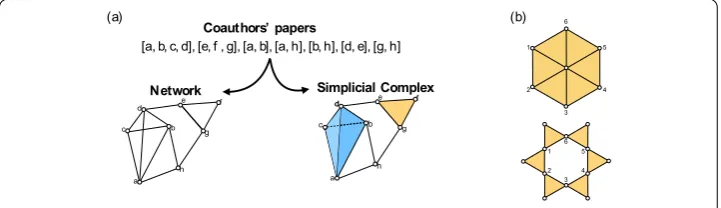
To gain an intuitive understanding of the differences between a network and a simplicial representation of the same data, consider the following toy example. Let us imagine that we are given seven papers with the following list of author sets:
[a,b,c,d], [e,f,g], [a,b], [a,h], [b,h], [d,e], [g,h]
as shown in Figure . Consider first the papers [a,b], [b,h], [a,h]. These three papers from a network point of view create a triangle. However, also the paper [a,b,h] would be described as the corresponding triangle in a co-authorship network. Adopting a sim-plicial language instead, we have immediately access to a richer interactions codebook from which to choose: the three papers [a,b], [b,h], [a,h] are mapped in a set of three -simplices (as defined by their author set), while the paper [e,f,g] is a -simplex is defined by its three authors and represented as a filled triangle. Already in such a simple example, we see that simplices and simplicial complexes are able to capture richer and more varied layouts as compared with networks.
Note that, while cliques are closely related to the concept of simplices, the latter retain a deeper descriptive power. Indeed, it is easy to see that, when comparing a simplicial and a network description of the same data, each (k– )-simplex in the simplicial complex will
Figure 1 Simplicial complexes vs networks.The figure shows the advantages of the simplicial compared to a network approach. A co-authorship dataset can be encoded both as a network, and as a simplicial complex(a). It easy to see how the simplicial complex approach are able to capture a richer layouts compared with networks. In fact the three papers[a,b],[a,h],[b,h]are mapped in an empty triangle in the simplicial complex, while the single paper[e,f,g]is represented as a filled triangle. This difference is crucial in the detection of holes in the simplicial complex. In both cases depicted in(b)the cycle
be associated with ak-clique on the same vertices in the network. However, the converse is not true: not everyk-clique in the network corresponds to a (k– )-simplex in the complex, just like the three edges in Figure do not correspond to the filled triangle. This is a direct example of how high-order information cannot always be reconstructed from lower-order interactions.
3.2 Simplicial measures
Simplicial complexes provide access to a larger set of local and mesoscopic observables. At the local level, we focus on two main features of the simplicial complexes: the distribution
P(s) of sizessof facets (maximal simplices); and the distributionP(d) ofsimplicial degree dof authors, defined as the number of facets that an author belongs to.
We can also ask new questions: for example, we can study a simplicial version of struc-tural holes []. Where at the network level one looks for how many of the existing wedges are closed by a third edge, hence probing the local clustering structure, at the simplicial level we can ask how many of the set of three edges (-simplices) that are arranged in a triangle are covered by a full triangle (-simplex). The two possibilities are shown in Fig-ure (a), where we see that the authorse,f,gcollaborated together on one paper, while the authorsa,b,hpublished in pairs, but never all of them together. Therefore measuring the number of filled triangles over the total number of possible triangles measures how much collaborations are integrated in a given field. Note also that this distinction could not have been made using the network projection (shown too in Figure ).
Configurations like the empty triangle just described, and more general pattern of dis-connectivity, are captured by the homology of a simplicial complex. Homology can be thought intuitively as the study of the holes in all dimensions of a certain dataset, and then implicitly of its shape. It provides a representation of the dataset complementary to that obtained by looking only at the dense regions (communities), and which is impossible to obtain from k-clique decompositions or other standard network methods [, ]. To compute homology means to detect and identify the empty spaces that are bounded by
k-simplices. At low dimensions the results can be easily interpreted as connected compo-nents and holes in the simplicial complex, but higher-order cavities can be of more difficult interpretation.
We are going to focus on the study of -dimensional homological cycles, i.e. two-dimensional holes bounded by edges, of the co-authorship simplicial complex. Homology is not only limited to small cycles (like triangles), but can probe larger holes which span significant parts of a simplicial complex. These features give a unique prospective, since they represent the cycles in the network (cordless closed paths) which cannot be reduced to a point when collapsing all the -simplices (triangles) in the simplex. This fundamental property is depicted in Figure . The two complexes in Figure (b) are composed by the same facets (the six full triangles). They have however a different shape (or technically, one-dimensional homology): the top one is essentially a large disk and can be contracted to a point, while the bottom one is akin to a ring, since the simplices bound an empty cy-cle. Note also that the cycle[0,1,2,3,4,5]is cordless in both cases, but only in the bottom case it cannot be contracted and hence it corresponds to meaningful information. In this sense, it provides mesoscopic information and we will use it to study the shape of the co-authorship simplicial complexes at different scales.
possible closed paths of length three. This gives us a higher-order notion of structural co-hesiveness, inspired by that of structural holes, but informed by homological information. We dub this measuresimplicial closurefor short. We then consider all the -dimensional homological cycles and analyze their trajectories through the simplicial complex. As by definition homological cycles bound holes, we study how they link dense parts of the complex together. In order to do this, we detect communities (using InfoMap []) on the simplicial complex and study how cycles link different communities with each other.
Note also that we ignore the quantity of papers published by the same group of authors, acknowledging only their collaboration as a simplex in the simplicial complex. Naturally, repeated collaborations - similarly to collaboration networks - can be encoded by assigning weights to simplices. In this case one would need to employ a parameterized version of homology, called persistent homology, which allows to deal with weighted simplices, as for example was done in []. However, we found that in our dataset adding weights did not yield significant additional information and thus restricted ourselves to an unweighted representation.
.. Simplicial contraction and complexity reduction
The rich information encoded in simplicial complexes comes at the expense of an in-creased computational cost. Although storing a simplicial complex as a list of facets is extremely parsimonious, the calculation of homology requires to list all the possible sub-sets. Therefore, even though the algorithm is polynomial, it can be very impractical when working with large simplices. This is due to the fact that each (s– )-facet gives rise to s simplices and thus the complexity of the computation of homology scales exponentially with the dimension of the simplicial complexO(m) >O([δ]), wheremis the number
of simplices in the simplicial complex, andδ is its dimension. This prevents us from di-rectly computing the homology of systems where large simplices are present - as is the case of the whole arXiv dataset. It is however possible to solve this exponential escalation in complexity and memory usage by studying an appropriately reduced but similar simplicial complex: we take inspiration here from the tidy set [] and the simplicial strong collapse [] to build a new simplicial complex, which contains fewer simplices but has the same homology groups. Each facet of the original simplicial complexKis represented by a node in a new oneχ(K), andk+ nodes inχ(K) span ak-simplex if the corresponding facets have at least one node (author) in common. The simplicial complex created this way is homologically equivalent to the original one due to the nerve theorem []. In fact, the complexχ(K) is what in mathematics is defined as the nerve of an open covering - in this case, the simplicial complexKbestowed with the Alexandrov topology []. We illustrate the transformation with a toy example in Figure .
The correspondenceχ:K→χ(K) described above however does not guarantee auto-matically thatχ(K) will have fewer simplices as compared with the original one. Indeed, it is possible to build simple examples showing a decided increase of the number of simplices after the transformation, e.g. consider a simplicial complex composed by many simplices all attached by a single node, which when transformed will yield a new simplicial com-plex with a simcom-plex of dimension the original node’s simplicial degree. More generally, if
Figure 2 Reduction of simplicial complex size. The figure shows an example of simplicial complex (a)and its correspondent dual complex(b). Each facet of the original simplicial complex is represented by a node in the dual complex, andk+ 1 nodes span ak-simplex if the correspondingk+ 1 facets have at least a node in common. In both simplicial complexes, the facets are colored according to their dimension. It is easy to see that applying the
complexity reduction to the simplicial complex(a)reduces the total number of simplices from 91 to 28, while fixing the homology (both complexes have one connected component, and one hole (1-dimensional cycle).
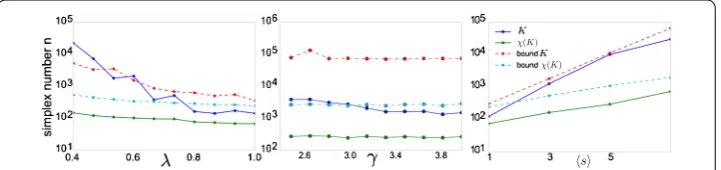
Figure 3 Performance of reduction of simplicial complex size.The panels show the total simplex number (solid lines) and the upper bound (dashed lines) for simplicial complexes built with facet size sequence sampled from the exponential (left), Zipf distribution (middle) and Poisson (right). On thex-axis we plot (from left to right) the power law exponentγ, the average valueλand the exponentν. It is easy to see that in all cases and for a range of parameters there is a large reduction in simplex number going fromKtoχ(K). Moreover, the bounds onn(K) andn(χ(K)), although not tight, reflects closely that betweenn(K) andn(χ(K)) and can therefore be used as a good proxy to decide whether applying the simplicial reductionχis appropriate or not.
ssimplices and thus the number of simplicesn(K) of a simplicial complexKwith facet size sequence{k}is bounded by{s}s, which for largesis dominated by maxs. Under the transformationχeach node inKbecomes a (d– )-simplex inχ(K), hence a first heuristic to performχis thatmaxsmaxd.
This criterion relies on the fact that the presence of large tails in the facet size distribu-tion will create a very large number of simplices if one does not transform toχ(K). In Fig-ure we give evidence for this by generating random simplicial complexes with facet size taken from a three different distributions: exponential (p(x)∼e–x/ν), Zipf ’s (p(x)∼x–γ)
and Poisson (p(x)∼λxe–x/x!). In all cases, we find a reduction of a few orders of magnitude ofngoing fromKtoχ(K). As expected, we also find the largest reductionn(K)/n(χ(K)) happening when the facet size distributionf(K) is characterized by longer tails (respec-tively lowerγ for Zipf, largerλfor Poisson and smallerν for exponential), as the tails represent large facets inKthat are mapped to a single point inχ(K).
3.3 Information-theoretic comparison of size distributions
In order to assess whether two categories share common statistical properties - for exam-ple of their facets or degrees - we need a robust measure of the distance between distri-butions. Here we adopt the Jensen-Shannon Divergence [] (JSD) that for two distribu-tionsPandQis defined as:JSD(P,Q) =DKL(P|M) +DKL(Q|M), whereM=P+Qand
DKL(P|Q) = –xP(x)logQP((xx)) is the Kullback-Leibler divergence. It is easy to see how this
In our case, we will need to compare distributions defined on very different supports, e.g. the facet size distributions of mathandhep-ex. Moreover, we want to compare the different functional dependencies of the distributions we are testing, rather than how different their supports are. So for all the JSD results, we first map both distributions from their original supports to the support (, ) in the natural way and then calculate the JSD between the two distributions.
4 Results
4.1 Summary statistics
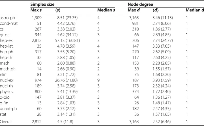
Table gives a summary of some of the characteristics of the categories of the arXiv data set and in Figures and we show respectively the facet size and simplicial degree dis-tributions for all categories. Excluding the two experimental physics categorieshep-ex, nucl-ex, we find that the average number of authors on a paper for the entire arXiv dataset iss = . with a standard deviation ofσs= ., which is consistent with the val-ues ofs obtained by restricting to individual categories. We also remark that the standard deviations and medians ofsare smaller for the mathematical disciplines, highlighting the known patterns of small collaborations in mathematics [].
Unsurprisingly, the two outliers,hep-exandnucl-ex, have very larges andσs, likely due to large-scale experiments (e.g. the The STAR Experiment in Brookhaven National Laboratory, or the ATLAS experiment in CERN). They however display different median
svalues, forhep-exand fornucl-exsuggesting that most of the collaborations are smaller in experimental high energy physics than in nuclear physics.
The average number of disjoint collaborations an author belongs to, described by the au-thor’s simplicial degree, isd = ., with standard deviationσd= ., and is consistent across all categories, with the exception ofhep-ex. Moreover, we also find coefficient of variation across categories forcv(d ) = . is much smaller than fors and the number of papers and authors (cv(s ) = .,cv(# papers) = .,cv(# authors) = .). We also find
Table 2 Facet and simplicial degree statistics. For each category we show the maximum, mean (with standard deviation), and median of the facet and simplicial degree sequences
Simplex size Node degree
Maxs s Medians Maxd d Mediand
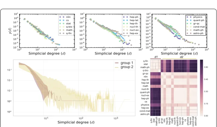
Figure 4 Comparison of facet size distributions.We show the facet size distributions (top) and their Jensen-Shannon divergence (bottom right) for all categories, ordered by maxsvalue. We find three main blocks of categories, which we highlight with different colors (bottom left).
Figure 5 Comparison of simplicial degree distributions.We show the simplicial degree distributions (top) and their Jensen-Shannon divergence (bottom right) for all categories, ordered by maxdvalue. As opposed to the facet distributions, we find two main groups of categories, which we highlight with different colors (bottom left).
that, while most papers are written by small groups of authors (mediansaround - for most categories), a large number of authors belongs to a single collaboration (mediand= for all categories).
4.2 Facet and simplicial degree distributions
of authors with a large number of different collaborations. In order to quantify the sim-ilarities among categories in terms of their facet and degree profiles we calculated the Jensen-Shannon divergence (JSD) [] between all pairs of distributions as described in the Methods section. If we order the categories by increasingmaxs, three groups can be clearly identified (Figure (bottom right)), highlighting that the three differentP(s) pro-files correspond to categories characterized by progressively largerssupport. In particular, the group characterized by smallmaxscontains the more mathematical categories ( hep-th,q-fin,math-ph,stat), while the one characterized by largemaxscontains the experimental and high-energy physics categories (hep-ph, physics, gr-qc, nucl-ex,astro-ph,hep-ex). In Figure (bottom left) we plot for each group the envelop of the distributions of the corresponding categories. In Figure we report the results of the same analysis for the simplicial degree distributions. In this case in Figure (bottom right) we ordered the categories by increasingmaxd, highlighting the presence of two cat-egory subgroups, a small one containingq-fin,stat,math-ph,q-bio, the second one containing the others. We also observe that the JSD values between the facet size distri-butions (Figure (bottom right)) are consistently larger (of about an order of magnitude) than those between the simplicial degree distributions (Figure (bottom right)), implying that the simplicial degree distributions are much closer to each other than the facet size ones.
4.3 Simplicial closure, large-scale structure and homological cycles
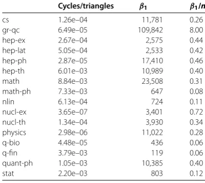
We are interested in probing both the local and the large scale structure - orshape, in short - of co-authorship data. In general, this has been done by finding communities or dense subgraphs which are generally thought to represent specific disciplines or subfields. How-ever, this approach does not provide information about how such communities relate to each other. To investigate these relationships, for all categories we computed the homol-ogy of the associated simplicial complexes, that is we found all the (homological) cycles, as described in Figure . In Table we report the results for the number of one-dimensional cycles in each complex.
We focus first on the shortest possible cycles, triangles. We find that the fraction of cycles of length that are not covered by a full triangle (-simplex) is very small for all categories, ranging between – fornucl-exand∼– formath. In other words, adapting the term from the network literature [], we can say that we find evidence of a very strong simplicial closure: in the great majority of cases whenever three authors have collaborated in pairs, they also have collaborated on a paper together.
One might expect this to be related to the number of cycles,β, present in the simplicial
complex, with a larger abundance of cycles implying a smaller triadic closure. However, we find no significant correlation between the ratio of open triangles to closed triangles and the total number of cycles (p> . for Spearman correlation). Interestingly, we find instead a negative (Spearman) significant correlation (p= .) between the number of open triangles and the ratioβ/nof overall number of cyclesβand the number of facets
nof the category’s simplicial complex.
We move our attention now to all homological cycles, not only the short ones. In Figure we report the distribution of cycle lengths for all categories, shown in order of growing values ofβ/n. The JSD matrix shows again a clean -block structure once it is ordered by
Table 3 Analytics on Homological cycles. For each category we show the number of cycles in the graph (β1),β1divided byn, the total number of authors in each category, and the
percentage of triangles in the graph that don’t satisfy triadic closure, that is # cycles of length 3
# triangles in the graph. Note that by number of triangles in the graph we mean the number of closed paths of length three in the co-authorship network
Cycles/triangles β1 β1/n
cs 1.26e–04 11,781 0.26 gr-qc 6.49e–05 109,842 8.00 hep-ex 2.67e–04 2,575 0.44 hep-lat 5.05e–04 2,533 0.42 hep-ph 2.87e–05 17,410 0.46 hep-th 6.01e–03 10,989 0.40 math 8.84e–03 23,508 0.31 math-ph 7.33e–03 647 0.08 nlin 6.13e–04 724 0.11 nucl-ex 3.65e–07 3,401 0.72 nucl-th 1.34e–04 3,930 0.34 physics 2.98e–06 11,022 0.28 q-bio 4.48e–05 436 0.06 q-fin 3.79e–03 119 0.06 quant-ph 1.05e–03 10,385 0.40 stat 2.20e–03 803 0.12
Figure 6 Cumulative distributions of cycle length.We show the cycle length distributions (top) and their Jensen-Shannon divergence (bottom right) for all categories, ordered byβ1/nvalue. We find two main groups of categories, which we highlight with different colors (bottom left). We groups categories in the subplots by growing values ofβ1/n(top, from left to right) and note that as the cycle sparsity increases, the maximum cycle length decreases.
gr-qc,nucl-ex), with a narrower distribution of cycle lengths, and a second with all the other categories displaying cycle length distributions with broader tails. We observe that the categories in the first group also display generally strong simplicial closure.
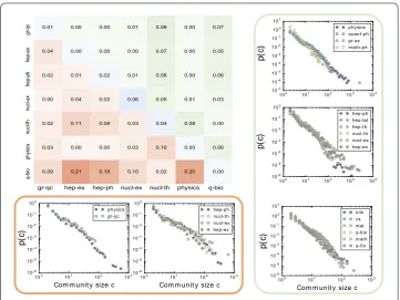
Figure 7 Distribution of community sizes.In the green box, we plot the community size distributions obtained from the underlying graph of the original simplicial complex. In the red box, we plot the community size distributions for the categories for which we performed the simplicial reduction. The central matrix shows: the JSD between the community size distributions of the original categories (green cells, upper triangular matrix), the JSD between the community size distributions for the transformed complexes (red cells, lower triangular matrix), and the JSD between the size community size distributions of the categories before and after the reduction. In all cases we find that the differences between the various distributions are small (JSD is defined in (0, log 2)).
communities a cycle traverses as a function of its length. However, forgr-qc,hep-ex, hep-ph,nucl-ex,nucl-th,physics,q-biowe need to perform the simplicial
re-duction (described in Section ..) to calculate the homology. Therefore, we detected the communities also on the transformed simplicial complexes. In Figure we show the community size distributions for all categories in the green box, and for the transformed categories in the red box. We found that overall the community size distributions are very similar across all categories (average JSD across all pairs .). Also, for the categories that underwent the simplicial reduction, we find a very small distance between the distribu-tions before and after the reduction (blue diagonal of matrix in Figure ). Additionally, we find a small accentuation of the distances between community size distributions for categories. This can be seen by comparing the symmetric elements in the green and red shaded regions of the matrix of Figure . Despite this the most distributions are still very close after the transformation.
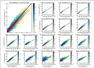
Figure 8 Cycles and community counts.Color intensity represents the number of cycles of length linking
ncommunities. Red dashed lines represent the upper bound on the number of traversed communities, while black dashed lines the random expectation. We provide also a linear fit to the data (black solid lines, with confidence intervals) showing that cycles are strongly associated with community bridging.
actually bridging between communities or not. In Figure we plot the diagonal as the up-per bound on the number of communities a cycle can cross (a cycle cannot traverse more communities that the number of its nodes) and the expected number of communities a cycle of given length should traverse (black dashed line) as a proxy for whether cycles tend to bridge between communities or not. We find indeed that in all case the number of communities traversed by each cycle is much larger than random expectation, confirm-ing their role as important features linkconfirm-ing together different regions of the collaboration simplex.
5 Discussion
We also identified three groups of categories on the basis of their different functional forms forP(s). Although the JSD differences are obtained in a way as to make them inde-pendent from the size of the category or of itsmaxs, we find that indeed the maximums
of a category predicts well the blocks observed in Figure . This is also reminding of the observations made in [, ] about the performance of teams of small, medium and large size. In our dataset, we do not have measures of performance, hence we cannot make a direct link between a category’s structural properties and its success. However, we do see the group’sP(s) change functional form, becoming broader and broader, as we move from group s to group s (Figure ), highlighting different organizational structures likely due to the different topics (e.g. group s is mainly theoretical work, s is mainly experimental work).
In fact, these results suggest that authors in experimental categories tend to collaborate in more large and not fully overlapping groups. Again, thinking about the dynamics of large experiments, this is reasonable since they acquire new authors and lose others over time leading to different facets, whereas the lower number of papers that are also facets in the most theoretical aspects of the same disciplines implies a slower turnover of members in time, and smaller repeated collaborations within larger groups.
We also introduced a simplicial analog of the triadic closure, simplicial closure, which could not be defined using networks or cliques alone. We found a very strong closure in all categories, which implies that - with high probability - a triple of authors that collab-orated in pairs will also collaborate as a group. This cohesiveness indicates the presence of a higher-order clustering: instead of creating a link to the friend of my friend, what we are seeing here is that the three of us become a group of three. Note also that this ob-servation is possible because we are adopting a simplicial description. Interestingly, this type of structural cohesiveness is consistent with what one would expect in models of lo-cal growth by copying previously reported for co-authorship and social networks [, ]. However, the patterns of local cohesiveness did not correlate with the number of authors or the size of collaborations. Interestingly, we also found that the local cycle structure does not correlate with the large-scale (homological) cycle structure, encoded in the cycle length distributions and inβ/n. For example, the group of categories characterized by
narrower cycle length distribution (blue distribution in Figure ) have very different sim-plicial closure values. These observations are consistent with local growth mechanisms that are responsible for the local dense patterns but cannot justify the large scale cycles that, instead, we find link together communities across the whole complex, acting as a scaffold [] supporting the dense communities, again highlighting a difference between the (quasi)-local structure and the large-scale structure, possibly organized along funding and academic leadership lines [, ].
of infrastructural or organizational constraints [], which would likely benefit from a simplicial modeling. This would also open the door to generalizations of our observations to the case of weighted simplices, which could be achieved with a persistent homology approach [], and to the inclusion of temporal features of the network, which again could find a likely phrased within the framework of zigzag homology [].
Acknowledgements
We thank the anonymous reviewers for their constructive comments and J.-G. Young for collecting and sharing the arXiv dataset for this study.
Funding
GP and AP acknowledge the support of the ADnD project by Compagnia San Paolo. FV acknowledge the support of the Laboratorio Lagrange project by Fondazione CRT.
Availability of data and materials
Due to the size, the raw dataset used is freely available upon request from the corresponding author.
Competing interests
The authors declare that they have no competing interests.
Authors’ contributions
AP, FV and GP conceived and designed the study, performed the analysis and wrote the manuscript. All authors read and approved the final manuscript.
Publisher’s Note
Springer Nature remains neutral with regard to jurisdictional claims in published maps and institutional affiliations.
Received: 8 March 2017 Accepted: 15 August 2017 References
1. Clarke BL (1964) Multiple authorship trends in scientific papers. Science 143(3608):822-824
2. Clarke BL (1967) Communication patterns of biomedical scientists. I. Multiple authorship and sponsorship of federal program volunteer papers. Fed Proc 26:1288-1292
3. Newman ME (2001) The structure of scientific collaboration networks. Proc Natl Acad Sci USA 98(2):404-409 4. Girvan M, Newman ME (2002) Community structure in social and biological networks. Proc Natl Acad Sci USA
99(12):7821-7826
5. Palla G, Barabási A-L, Vicsek T (2007) Quantifying social group evolution. Nature 446(7136):664-667
6. Börner K, Contractor N, Falk-Krzesinski HJ, Fiore SM, Hall KL, Keyton J, Spring B, Stokols D, Trochim W, Uzzi B (2010) A multi-level systems perspective for the science of team science. Sci Transl Med 2(49):49cm24
7. Glänzel W, Schubert A (2004) Analysing scientific networks through co-authorship. In: Handbook of quantitative science and technology research. Springer, Berlin, pp 257-276
8. Bettencourt LM, Kaur J (2011) Evolution and structure of sustainability science. Proc Natl Acad Sci USA 108(49):19540-19545
9. Palla G, Derényi I, Farkas I, Vicsek T (2005) Uncovering the overlapping community structure of complex networks in nature and society. Nature 435(7043):814-818
10. Ruan J, Zhang W (2008) Identifying network communities with a high resolution. Phys Rev E 77(1):016104 11. Sales-Pardo M, Guimera R, Moreira AA, Amaral LAN (2007) Extracting the hierarchical organization of complex
systems. Proc Natl Acad Sci USA 104(39):15224-15229
12. Coccia M, Wang L (2016) Evolution and convergence of the patterns of international scientific collaboration. Proc Natl Acad Sci USA 113(8):2057-2061
13. Lancichinetti A, Fortunato S, Kertész J (2009) Detecting the overlapping and hierarchical community structure in complex networks. New J Phys 11(3):033015
14. Guimera R, Uzzi B, Spiro J, Amaral LAN (2005) Team assembly mechanisms determine collaboration network structure and team performance. Science 308(5722):697-702
15. Castellano C, Fortunato S, Loreto V (2009) Statistical physics of social dynamics. Rev Mod Phys 81(2):591 16. Börner K, Dall’Asta L, Ke W, Vespignani A (2005) Studying the emerging global brain: analyzing and visualizing the
impact of co-authorship teams. Complexity 10(4):57-67
17. Wagner CS, Leydesdorff L (2005) Network structure, self-organization, and the growth of international collaboration in science. Res Policy 34(10):1608-1618
18. Pan RK, Saramäki J (2012) The strength of strong ties in scientific collaboration networks. Europhys Lett 97(1):18007 19. Milojevi´c S (2014) Principles of scientific research team formation and evolution. Proc Natl Acad Sci USA
111(11):3984-3989
20. Kenna R, Berche B (2012) Managing research quality: critical mass and optimal academic research group size. IMA J Manag Math 23(2):195-207
21. Derényi I, Palla G, Vicsek T (2005) Clique percolation in random networks. Phys Rev Lett 94(16):160202
23. Weinberger S (2011) What is. . . persistent homology? Not Am Math Soc 58(1):36-39 24. Patania A, Vaccarino F, Petri G (2017) Topological analysis of data. EPJ Data Sci 6(1):7 25. Hatcher A (2002) Algebraic topology. Cambridge University Press, Cambridge
26. Vejdemo-Johansson M, Skraba P (2016) Topology, big data and optimization. In: Big data optimization: recent developments and challenges. Springer, Berlin, pp 147-176
27. Pastor-Satorras R, Castellano C, Van Mieghem P, Vespignani A (2015) Epidemic processes in complex networks. Rev Mod Phys 87(3):925
28. Liu Y-Y, Barabási A-L (2016) Control principles of complex systems. Rev Mod Phys 88(3):035006 29. Burt RS (2009) Structural holes: the social structure of competition. Harvard University Press, Cambridge 30. Ghrist R (2008) Barcodes: the persistent topology of data. Bull Am Math Soc 45(1):61-75.
doi:10.1090/S0273-0979-07-01191-3
31. Carstens C, Horadam K (2013) Persistent homology of collaboration networks. Math Probl Eng 2013:815035 32. Rosvall M, Bergstrom CT (2008) Maps of random walks on complex networks reveal community structure. Proc Natl
Acad Sci USA 105(4):1118-1123
33. Zomorodian A (2010) The tidy set: a minimal simplicial set for computing homology of clique complexes. In: Proceedings of the twenty-sixth annual symposium on computational geometry. ACM, New York, pp 257-266 34. Wilkerson AC, Moore TJ, Swami A, Krim H (2013) Simplifying the homology of networks via strong collapses. In: 2013
IEEE international conference on acoustics, speech and signal processing (ICASSP). IEEE, pp 5258-5262 35. Lin J (1991) Divergence measures based on the Shannon entropy. IEEE Trans Inf Theory 37(1):145-151 36. Newman ME (2004) Coauthorship networks and patterns of scientific collaboration. Proc Natl Acad Sci USA
101(Suppl 1):5200-5205
37. Kenna R, Berche B (2011) Critical mass and the dependency of research quality on group size. Scientometrics 86(2):527-540
38. Krapivsky PL, Redner S (2005) Network growth by copying. Phys Rev E 71(3):036118
39. Szulanski G, Jensen RJ (2008) Growing through copying: the negative consequences of innovation on franchise network growth. Res Policy 37(10):1732-1741
40. Petri G, Expert P, Turkheimer F, Carhart-Harris R, Nutt D, Hellyer PJ, Vaccarino F (2014) Homological scaffolds of brain functional networks. J R Soc Interface 11(101):20140873. doi:10.1098/rsif.2014.0873
41. Carayol N, Matt M (2006) Individual and collective determinants of academic scientists’ productivity. Inf Econ Policy 18(1):55-72
42. Petri G, Scolamiero M, Donato I, Vaccarino F (2013) Topological strata of weighted complex networks. PLoS ONE 8(6):66506. doi:10.1371/journal.pone.0066506
43. Bianconi G, Rahmede C, Wu Z (2015) Complex quantum network geometries: evolution and phase transitions. Phys Rev E 92(2):022815
44. Courtney OT, Bianconi G (2017) Weighted growing simplicial complexes. arXiv:1703.01187
45. Young J-G, Petri G, Vaccarino F, Patania A (2017) Construction of and efficient sampling from the simplicial configuration model. arXiv:1705.10298
46. Wu Z, Menichetti G, Rahmede C, Bianconi G (2015) Emergent complex network geometry. Sci Rep 5:10073 47. Ponds R (2009) The limits to internationalization of scientific research collaboration. J Technol Transf 34(1):76-94 48. Carlsson G, De Silva V, Morozov D (2009) Zigzag persistent homology and real-valued functions. In: Proceedings of