DOI 10.1007/s13173-013-0105-y O R I G I NA L PA P E R
Characterizing the communication in the Amazon rainforest:
towards a realistic simulation
Afonso D. Ribas· Antonio R. Carvalho Jr. · Carlos M. S. Figueiredo · Eduardo F. Nakamura
Received: 24 January 2012 / Accepted: 4 March 2013 / Published online: 2 April 2013 © The Brazilian Computer Society 2013
Abstract Many literature papers evaluate solutions in wireless sensor networks by simulation experiments. How-ever, little attention is given to the adequacy of the simulator propagation models to the environment in which such solu-tions are employed. This can lead to imprecise or inconsis-tent results in relation to the real world. This paper presents a methodology for adjusting the parameters of these models. In particular, we present experimental results for rainforest environments, which can be the goal of many sensor net-works monitoring applications. The impact of the proposed approach is shown by evaluating a localization solution. The results show that this procedure is necessary for a higher fidelity of simulation experiments.
Keywords Propagation·Experimentation·Simulation
1 Introduction
Many research efforts are being dedicated to the wireless sensor networks (WSNs) [3] in the last few years. This is due to their capacity to increase the way we interact with the
A. D. Ribas (
B
)·A. R. Carvalho Jr.·C. M. S. Figueiredo· E. F. NakamuraComputer Science Lab, Research and Technological Innovation Center (FUCAPI), Danilo Areosa de Matos, 381, Manaus, AM 69075-351, Brazil
e-mail: [email protected] A. R. Carvalho Jr.
e-mail: [email protected] C. M. S. Figueiredo
e-mail: [email protected] E. F. Nakamura
Federal University of Amazone (UFAM), Manaus, Brazil e-mail: [email protected]
world. In particular, many environmental monitoring appli-cations are under study [7], and they are being employed in environments with very distinct characteristics which affect the wireless communication. Particularly, many researchers in Brazil and all over the world are concerned about Amazon rainforest monitoring for studies and preservation due to its dimension and biodiversity.
In the initial phase of the WSN’s development many solu-tions were proposed under conceptual aspects with strong use of experimentation by simulation. These are solutions such as protocols and algorithms for MAC [30], routing [4], local-ization [9], and many others which depends on the wireless communication and the channel characteristics. Obviously, not all the scenario characteristics and premises considered in these works are observed in practice, as shown by recent work [13], and disparities between simulations and real plat-forms become clear [11,25].
As a result, many papers have focused on the exper-imentation of wireless radios within different scenarios [5,6,21,34,41,43]. The main goal is to evaluate how the signal strength and delivery ratio are affected by distance and obstacles. However, simulation is still important for the development of new solutions, because not always there is an infrastructure favorable for practical experimentation, besides the cost and time necessary for this. Thus, we show a methodology to characterize the communication in the Amazon rainforest, which is a very distinct environ-ment from those studied in literature, based on practical experiments.
minimization we estimated the parameters of the Shadow-ing propagation model, which is very common in the exist-ing simulation suites. Then, we used a localization system simulation in NS-21based on a multilateration algorithm to compare the obtained results against default parameters nor-mally used in simulations, and other parameters suggested in the literature. We show that fine tuning these parame-ters is necessary to represent what we can obtain in real experiments.
The remainder of the paper is organized as follows. Some theoretical fundamentals are introduced in Sect.2. Section3 presents the related work. In Sect. 4, we characterize the rainforest scenario. Section5discusses realistic simulation. Finally, our conclusions and future work are presented in Sect.6.
2 Background
2.1 Propagation models
The propagation models are traditionally used to predict the average signal strength (power) received at a certain distance of the transmitter, beyond intensity variability of signal in areas near a particular position. The simplest but representa-tive models are the Free Space and Shadowing. Both consider that path loss, the amount of power lost for the medium, is proportional to the distance between transmitter and receiver to the power of N, i.e.,
PL(d)∝dN, (1)
where d is the distance and N is path loss exponent that indicates the power decay rate with the distance. For the Free Space model, N is 2, and for the Shadowing model, Nranges from 1.5 to 6. The higherN is, the more severe is the environment for communication.
The Free Space model is used only when there is a vision path clearing between the transmitter and receiver. The Shad-owing model is used when there are many obstacles for prop-agation that is difficult to model into equations.
Other models take into account the effects of reflection, diffraction, and scattering [33]. The Two-Ray Ground model [19] deals with ground reflection, useful for predicting signal strength over distances of several kilometers when transmit-ter and receiver use towers of different heights. Diffraction effect is treated by the Knife-edge Diffraction model [26,33] in cases where there is a hill or mountain between transmit-ter and receiver. The Radar Cross Section model [35] aims to model the impact of the diffused reflections produced when a radio wave impinges on a non-uniform surface like a build-ing.
1http://www.isi.edu/nsnam/ns/.
Some models are described for particular environments. The outdoor models, like Okumura–Hata [22] and Walfisch and Bertoni [39], are derived for urban areas usually asso-ciated with cellular systems. Foliage or vegetation models estimate the path loss due to propagation though trees and foliage [36]. In this category we have Weissberger’s modified exponential decay model [40], ITU Vegetation model [24], COST235 model [2]. Generically, these models estimate the additional lossLby the expression:
Lveg=α× fβ ×dγ, (2)
where f is the frequency,dis the depth of the foliage along the line-of-sight path. Constantsα, β, andγare empirically calculated in each model. In spite of these models considering tree and foliage, they are not suitable for modeling propaga-tion when small and low-power radios are employed inside forests for short distances.
In this work, we use the Shadowing model to estimate path loss and received power in the Amazon rainforest. Next, we describe in detail this model and justify this choice. In addition, we also provide the theory of the Free Space model, once it may be used as base for many models including the Shadowing model.
2.1.1 Free Space propagation model
The Free Space model is used to predict received signal strength when the transmitter and receiver have a clear, unob-structed line-of-sight path between them [33]. The received power by a receiver antenna in dBm is given by [18]
Pr(d)= P0−20 log(f)−20 log(d)+27.56, (3)
whereP0is the power at zero distance from the antenna, f is the signal frequency in MHz anddis the distance (in meters) from the antenna.
2.1.2 Shadowing propagation model
Propagation models like Free Space and Two-Ray Ground predict the signal power received as deterministic functions of distance. It represents the communication area as a perfect sphere, however the behavior of a received signal propagation is random and distributed log-normally around the mean. The randomness of the signal behavior is caused by changes in the environment that directly impact the signal power [33].
The Shadowing model is separated in two parts. The first part provides the average of received powers at a certain dis-tance. The second part, models the randomness of the signal at this distanced.
The received or input power is calculated as
whered is the distance between the receiver and the trans-mitter in m and Pt is the transmission power in dBm. The path loss, PL in dBm, at a distanced is calculated as [33]
PL(d) (dB)=PL(d0)+10Nlog
d d0
+Xσ, (5)
whered0is the nearby reference distance. PL(d0)is the aver-age path loss ford0or an assumption using the Free Space model. N is the exponent of the path loss that indicates the power decay rate with the distance.Xσ is a zero-mean Gaussian distributed random variable with standard devia-tionσ(in decibels).
Combining Eqs.4and5, we have
Pr(d)=P0−10Nlog
d d0
+Xσ, (6)
where
P0=Pt−PL(d0). (7)
The adoption of the Shadowing model in this work is moti-vated by many reasons. First, it considers attenuation of the signal due to distance, and interferences caused by obstacles which are observed in the measurements. Second, the foliage models are not suitable for communication with both trans-mitter and receiver inside the forest. Variations of these mod-els are adapted for plantation environments, but they consider trees as measurable or countable objects. In the Amazon rain-forest, the trees are very close to each other and there are many other obstacles, such as: roots, branches, lianas, shrubs, and to measure their depth is a difficult task. Third, the Shadow-ing model is simple, easy, generic, and popular. Many envi-ronments were characterized using this model [5,18,33,34] allowing comparison and reuse. Last, the Shadowing model is implemented by simulators like NS-2 and Castalia.2
3 Related work
Regarding wireless communication characterization, Zhao and Govindan [43] carried out experiments investigating the packet delivery in three different environments: an indoor office building, a habitat with moderate foliage, and an open parking lot. They showed that by varying the distance between nodes, we can identify regions in which the com-munication becomes unstable, the so-called “gray areas” or “transitional region”. Although they are trying to characterize wireless communication, they focused on packet delivery.
Zuniga and Krishnamachari [44] provided an extensive study about the “transitional region”. They identified the causes and derived expressions for its width and for the packet
2http://castalia.npc.nicta.com.au.
delivery rate. For increasing realism in simulation experi-ments, the authors recommend the characterization of the interested environment.
The relationship between packet delivery and received sig-nal strength indicator (RSSI) and link quality indicator (LQI) was investigated by Srinivasan and Levis [37]. Their exper-imental study showed that LQI actually is a better quality indicator than RSSI for a wider signal degradation range. However, the focus of this work was the RSSI itself, not characterization or realistic simulation.
Seidel and Rappaport [34] and Andersen et al. [5] have reported many contributions about propagation models, specifically about the Shadowing model and derivatives. Both have conducted a large number of experiments to model and characterize the wireless communications channels in indoor scenarios.
Some studies on propagation models for forest environ-ments have been presented in the literature since the 1960s until today [6,21,27,28,38]. Some of these studies focus on medium and high frequencies (2–200 MHz) [38], others on UWB (above 3.1 GHz) [6,28] and others only on theoretical analysis [27,28]. Except for Tamir’s work [38], the idea is to evaluate the impact of the forest on long-distance telecom-munication systems (over 1 km) when transmitter or receiver is outside of the forest. In this work, we evaluate the com-munication for ZigBee radios inside the forest, operating in 2.4 GHz, for short distances.
In the context of WSN, Ndzi et al. [31] and Mestre et al. [29] carried out experiments in plantations to evaluate vegetation attenuation models (discussed in Sect. 2.1) for precision agriculture.
Gay-Fernandez et al. [21] present a complete study for the deployment of a WSN in a forest in Spain based on ZigBee, including the propagation model analysis. They carried out some propagation experiments and found parameters for dif-ferent deployment situations. These parameters can be easily adapted to the Shadowing parameters. However, the environ-ment studied, even being a forest, presents features different from the Amazon rainforest which, basically, is denser than the Spanish forest. Thus, their parameters could not be used in applications in our context. One of our main objectives in this work is to characterize the communication in the Ama-zon rainforest.
of the incorrect tuning of propagation parameters in the NS-2 simulator for actual applications.
4 Rainforest scenario characterization
In this section we present the used methodology to charac-terize the Amazon rainforest scenario. First we carried out practical experiments to assess the behavior of current wire-less communication for actual applications. In the second part of characterization, we used the measured received power to estimate the parameters of the Shadowing propagation model for this scenario.
4.1 Experimentation
This part extends our previous work [20] by presenting new results and we tested another platform for comparison. In the following, we show the experimental methodology and results.
4.1.1 Test scenario
The experimentation was conducted in an underexplored rainforest area in which a WSN could be deployed for envi-ronmental monitoring. This scenario is defined by a small area inside a preservation area, in which the terrain is flat and we have several natural obstacles to signal propagation, such as a wide variety of trees, bushes and leaves (Fig.1a). This is a typical dense rainforest with low human interven-tion. We have experimented with sensor nodes positioned on the ground (Fig.1b). These nodes are deployed in an ad hoc and unplanned fashion (dropped on the ground) or by using autonomous mobile robots. Our previous work [20] showed the case where the nodes were positioned on a base 1.25 m from the ground. The results were similar with those we present here (in Sect.4.1.4), but with a higher communi-cation range.
4.1.2 Wireless sensor network platforms
We have chosen the Crossbow’s MicaZ [14] and Iris [15] as the evaluation platforms (Fig.2), for these belong to a popular sensor platform series that have been used in several proto-type applications. MicaZ and Iris represent a evolution com-pared to the previous representative, the Mica2. The MicaZ platform adopts the CC2420 radio [12] whereas Iris adopts the RF230 radio [8] both compliant with the IEEE 802.15.4 (ZigBee) standard [23]. Table1shows the main parameters provided by the manufacturer for both radios.
Both radios provide the RSSI and the LQI. The RSSI indi-cates the received power at the RF pins of the radio of received packets. The LQI indicates how good is the wireless link and can be affected by spectrum interferences and high noise
lev-(a)
(b)
Fig. 1 Rainforest scenario.aBroad view of the scenario.bNode’s placement detail
(a) (b)
Fig. 2 Evaluation platforms.aMicaZ Mote [14],bIris Mote [15]
els. The received power and LQI will be used as metrics in our experiments. Table2presents the manufacturer specifi-cations for both radios. According to the data-sheet of the Iris’s radio [8], the equation which converts RSSI to dBm is only valid for values between 1 and 28. A value of 0 indicates a received power less than−91 dBm.
Table 1 Transceivers main parameters (data-sheet [8,12,15,14])
Parameter MicaZ Iris
Transceiver CC2420 RF230
Radio frequency (GHz) 2.4 2.4
Bandwidth (kbps) 250 250
RF power (dBm) −24 to 0 −17.2 to 3 Receiver sensitivity (dBm) −94 −101 Outdoor comm. range (m) 75–100 >300 Indoor comm. range (m) 20–30 >50
Table 2 RSSI specifications (data-sheet [8,12])
Parameter CC2420 RF230
Dynamic range (dB) 100 81
Resolution (dB) 1 3
Register length (bits) 8 5
Values rangea −60 to 40 0 to 28
Power convers. equ.b −45+RSSI −91+3 (RSSI−1) aValues are registered in signed 2’s complement.
bPower in dBm.
value between 0 and 255. However, the CC2420 provides only an average correlation value (also known as a chip cor-relation indicator—CCI) of the eight first symbols of the received packet which can be combined with the RSSI to generate a LQI measurement by software. This correlation value varies between 50 and 110. Normally, only the average correlation value is used as LQI, and no additional process-ing is done [1,37]. For RF230, LQI values varies between 0 and 255 and is highly associated to an expected packet error rate (PER). A value of 255 indicates no frame error, whereas low values represent many erroneous received frames.
4.1.3 Test procedure
In every test round, the source node sends 20 packets to the sink node at a rate of 10 packets per s. We use the 20 trans-mitted packets to compute the delivery ratio.3 The trans-mission rate of 10 packets per s allows us to collect more data in less experimentation time without congestion in the network. By hardware limitations, we configured the output transmission power on 0 dBm for MicaZ and 0.5 dBm for Iris node. In addition, the sink node assesses the received power (obtained from the RSSI) and LQI for every packet. These three compose the set of metrics evaluated on the experiment. For each platform, we vary the distance between source and sink nodes, and in order to ensure the statistical relevance, we perform 33 rounds for every different platform.
3The percentage of packets received regarding the total packets sent by the source node.
Fig. 3 Delivery ratio variation according to the distance between nodes
4.1.4 Experimental results
Figure3a presents the relationship between the delivery ratio and the distance between source and sink nodes. We show all 33 values for each distance. Complementarily, we plot the average delivery ratio for every distance. For MicaZ nodes, the largest distance we could reach was only 6 m with about 30 % of delivery ratio (average). Iris nodes could reach 13.5 m with a high level of delivery ratio which can be explained by the “transitional region”, discussed in Sect.3. In this region, the communication becomes unstable due to the low signal-to-noise ratio (SNR) and presence of obstacles in such a con-figuration that contributes to the signal instead of degrading it. This phenomena is also observed at 10 m. Indeed, this region ranges from 7 to 13.5 m. Further than 13.5 m, no communication was observed.
Iris nodes reach larger distances than MicaZ because of the higher radio sensibility level (presented in Table1). For Iris node, significant obstacle4 produced local attenuations at 1.80 and 2.25 m.
For both platforms, we observe a great variation on the delivery ratio when the nodes’ distance was closer to the maximum distance we had attained, just like we observed in our previous work [20] and also reported by the literature [37,43] (discussed in Sect.3).
Figure 4a presents the received power values when we increase the distance between source and sink nodes. Once more, we show all 33 values for each scenario and the average values as well. Confirming the theory presented in Sect.2.1.2, the received power decreases with the distance until it reaches the radio sensibility (presented in Table1).
(a)
(b)
Fig. 4 Received power variation.aReceived power variation accord-ing to the distance between nodes.bRelationship between received power and delivery ratio
For Iris node, all the received power averages for distances greater than 7 m were−94 dBm. This saturation occurred because, at these distances, all the RSSI readings were zero indicating a received power lower than−91 dBm, according to the radio’s data-sheet [8]. In fact, we do not know the actual value for these distances, therefore, we plot on the graph the value−94 dBm which is the power calculated by the equation described in Table2when RSSI = 0. For many applications, such as localization systems, received power measurements are very important and are usually calculated using RSSI readings. Actually, using the Iris Mote, we only have relevant RSSI measurements (in range 1–28) when the distance is up to 6 m in the Amazon rainforest environment. For further distances we only have a “poor signal” indication. In addition, the delivery ratio is used by many routing algorithms as estimation of link quality for choosing routes.
(a)
(b)
Fig. 5 LQI variation. a LQI variation according to the distance between nodes.bRelationship between LQI and delivery ratio
In order to allow the comparison of the received power with the link quality, Fig.4b correlates the received power val-ues with the delivery ratio. We observe that when the signal strength is greater than a threshold (−90 dBm for MicaZ and
−94 dBm for Iris—or a RSSI indication of zero) we probably will have high delivery ratios. However, for smaller values, the received power quickly decreases and presents great vari-ations. This fact is also observed in other scenarios reported in different papers, such as Srinivasan and Levis [37] dis-cussed in Sect.3. Thus, we can conclude that RSSI may be used in all cases as a simple threshold for the link quality.
behavior is similar to the RSSI, i.e., it decreases according to the distance between nodes. Once again, we observed great variations in the LQI when the distance was close to the max-imum distance.
Comparing LQI variation with delivery ratio and received power variation, we observe that, for Iris nodes, the LQI is more related to the delivery ratio than received power (Figs.3, 5a). But, for MicaZ, LQI is more related to the received power (Figs.4a,5a). Figure5b supports this observation. Although the delivery ratio also presents great variation, for Iris nodes, this indicator is more representative than the received power, since such a variation is smoother for the LQI. For MicaZ nodes, we have a more abrupt variation with the decay of the indication around the value 75. As a link quality indica-tion, the LQI should be highly correlated with the delivery ratio instead of the received power. Thus, we can conclude that Iris’s LQI, although still far from ideal, is better than MicaZ’s. Moreover, the usage only of the average correla-tion value (CCI) as LQI is not recommended, requiring addi-tional calculation as suggests the manufacturer of MicaZ’s radio.
All these experiments reinforce the difficulty of using received power and LQI to represent the link quality and distance estimation. These factors are relevant as they have been considered by solutions for data routing and node local-ization that usually adopt imprecise theoretical values.
4.2 Shadowing model parameters estimation
After practical experiments, we had a database with collected pairs of average of received power and distance (pi,di). Using this database, we estimated the parameters of the Shadowing propagation model (described in Sect.2.1.2) for MicaZ and Iris nodes. Normally, theNcoefficient from Eq.6 varies between 1.5 and 6 and can be obtained by minimizing the MSE described as follows
MSE(N)= 1 k
k
i=1
[pi− ˆpi]2 (8)
where pi is a received power measured for a given distance
di.pˆi represents the estimated received power using a prop-agation model. For the Shadowing model,pˆi can be written as
ˆ
pi =P0−10Nlog
di
d0
. (9)
Note that Eq. 9 differs from Eq. 6 by the term Xσ which does not appear in Eq.9. It means that we only con-sider the deterministic part of the Shadowing model to esti-mate the received power. d0 was the shortest distance in the propagation experiment. P0 was the average measured power atd0.
According to Rappaport [33], the standard deviation σ from Eq.6can be calculated using the minimum mean square error (MMSE) found by:
σ =√MMSE. (10)
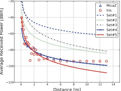
The estimated parameters were compared in Table3with parameters for others environments. The first set of parame-ters are the default values used in NS-2 [17]. The NS-2 is one of the most used simulators in WSNs for scale scenarios. Sets 2 and 3 represent the parameters for a Spanish forest with two different configurations [21]. Finally, the last two sets represent the estimated values in our practical experiments for MicaZ and Iris nodes. We have also added the MSE for MicaZ’s and Iris’ collected measurements of each set.
We can notice that the MSE of sets for MicaZ and Iris were close compared to the others sets. The sets 1, 2 and 3 were at least ten times greater than the Amazon Forest’s sets for the collected data. Acceptable set of parameters (those with low MSE) generally has both N and P0parameters approximate to the actual values for the samed0. This can be observed on the first four sets, where we had the same value ofd0but an unbalance on theNandP0parameters. For sets 4 and 5, thed0was different, but the others parameters were correctly balanced.
Figure6presents the collected pairs(pi,di)for both plat-forms. Complementarily, we plot the mean curves (discard-ing the random term Xσ from Eq.2.1.2) for the Shadowing propagation model using the sets of parameters from Table3. For Iris node, the values greater than 6 m were not considered for the regression and MSE calculation.
Although there is the difference of values in Table 3 between sets 4 and 5, the curves in Fig.6for these sets are roughly similar which can be verified by the low MSE val-ues. This indicates that the parameters are describing the environment instead of motes. If we keep the same basic
Table 3 Shadowing model parameters for some environments
Set Environment N σ(dBm) d0(m) P0(dBm) MSEMicaZ MSEIris
1 NS-2 default 2.0 4.0 1.0 −40.2 1,254 1,214
2 Spanish forest 1 2.55 7.29 1.0 −55.9 297 346
3 Spanish forest 2 3.43 6.04 1.0 −43.4 667 874
4 Amazon rainforestM 2.14 1.86 1.0 −75.2 3 32
5 Amazon rainforestI 3.21 5.23 0.1 −40.4 14 27
characteristics (frequency and transmission power), we will have similar results for the environment. Besides, the model focuses on path loss (according to Eq.5) allowing even the representation of different transmission powers. Actually, the unique parameter related to the device isσ, once a particular radio could use better components that are more immune to variations/noise. Further, designers of the radio can also pro-vide extra hardware to deal with this problem decreasing the sigma parameter. We also can see that the mean curves for the sets 1, 2 and 3 are far from the curves for our regression lines. This is in agreement with the high values of MSE showed in Table3. Clearly, we can observe that sets 1, 2 and 3 do not represent the characteristics of the Amazon rainforest.
4.3 Tuning propagation model parameters
In this section we provide the procedure for characterizing new environments and for adjusting the propagation model parameters in the NS-2 simulation tool. The goal is to find parameters for a given environment even though we do not understand all the details of its behavior. In other words, our concern is about the statistical behavior of the communica-tion/channel, not the particularities of the forest. The steps are:
1 Signal strength experimentationFirst, we need to col-lect RSSI readings in the region varying the transmitter– receiver distance (see Sect. 4.1.3). The more readings you collect, the more accurate and statistically relevant will be your results. We suggest at least 30 samples per distance. A good idea is to find the maximum commu-nication range, and then, take as many as possible mea-surements within this range. It is important to take note of the transmission powerPt.
2 Parameter estimation By using the steps described in Section 4.2, we estimate the Shadowing propagation model parameters N and σ. We need to consider the transmission powerPtused in the experimentation. 3 Simulator parameter adjustingIn the NS-2 simulator, we
set the earlier found shadowing propagation model para-metersN, σ, andd0in the TCL configuration file.5The parameterd0is the shortest distance between transmitter and receiver in the signal strength experiment.
5http://www.isi.edu/nsnam/ns/doc/node221.html.
5 Localization experiments
Many solutions for wireless communication are proposed in the literature and validated in simulation tools consider-ing erroneous or unrealistic assumptions. In this section, we show the impact of the incorrect tuning of the propagation parameters in a simulation tool. In the following, we describe the experiment.
After estimating the propagation model parameters, we carried out two experiments, both based on a localization application: (1) a practical experiment; and (2) a simula-tion experiment. This applicasimula-tion was chosen due to its rele-vance in monitoring and event detection systems using WSNs [9,10]. Hereafter, we use only the Iris platform in our analy-sis.
The practical experiment was implemented based on the localization system for indoor environment proposed by BluePass [16]. Four fixed nodes were placed at the corners of a square area of 4×4 m2in the Amazon rainforest. Another node, called mobile node, was placed inside this square area. Periodically, the fixed nodes send data to mobile node. The mobile node gets the RSSI values and stores the received power in a list. For every new received packet, we calculate a new average of input powers. So, we estimate the distances between fixed nodes and mobile node, using the following equation:
ˆ
di =10[P0+10Nlog(d0)−pi]/(10N), (11)
wheredˆiis the estimated distance from mobile node to a fixed nodei.P0,Nandd0are the Shadowing propagation model parameters. pi is the current average received power related to a packets received from fixed nodei. Using these distances we estimate the mobile node position, called ppos, using multilateration. For every new received packet, we reestimate
(a)
(b)
Fig. 8 Localization error versus number of packets. a Practical experiment—εp,bsimulation experiment—εs
ppos. We repeated this experiment for several mobile node positions and for every set of parameters from Table3.
The simulation experiment was conducted in a NS-2 sim-ulator. We configured the simulator with the same area, nodes position and other characteristics as we did in the practical experiment. We did the following changes with the NS-2 code:
• Setting of theP0parameter on the Shadowing model.
• Calculation of the Shadowing model power, at a certain distance, according to Eq.6in dBm.
• Implementation of the Iris rules for reading RSSI/ received power values.
The estimated mobile node position in the simulation experiment was calledspos. Thus, we calculate the
local-Fig. 9 Simulation precision error—εspversus number of packets
ization errorεaccording to the following equation:
ε=di st(mpos,epos), (12)
where mpos is the mobile node position and epos is the estimated position which can be apposorspos. The function di st(·)is the Euclidean distance between two points. Figure7 summarizes the results.εpindicates the localization error in practical experiment andεsthe error in simulation.εspwill be introduced later.
Figure8presents average localization error for practical and simulation experiment when we increase the number of packets used to calculate the average power. These graphs compare the error for the parameters from Table3, excluding the NS-2 default parameters that presented errors in order of kilometers. From this point on, the set of parameters 5 will be referred to asestimated parameters, and the sets 2 and 3 asliterature parameters.
In the practical experiment, our estimated parameters pre-sented the smallest error, less than 2 m whereas the others were around 35 m. We observe a stability of the error values and this is important because some localization systems try to reduce the errors accumulating and averaging readings. Figure8a shows that this procedure do not increase signifi-cantly the method precision.
We can consider a good simulator when its results are near to the practical results. Thus, to evaluate the simulation preci-sion we should analyze the error between the estimated node position in simulation and estimated position in a practical experiment. This error will be calledsimulation precision error—εsp(showed in Fig.7) and can be calculated as
εsp=di st(spos,ppos). (13)
Figure9shows theεsp when we increase the number of packets. We observe a low error in the experiments with the estimated parameters indicating that estimations in simula-tion were near to estimasimula-tions in practical experiments. This is an indication that we have a realistic simulation using the estimated parameters. The errors for the literature parame-ters were almost ten times greater than the length of one side of the square region used in the experiment.
6 Conclusion
This work presented experimental data for rainforest wire-less communication, and the adequacy of the parameters of the Shadowing propagation model common in simulation suites. This adequacy was achieved from the measurements of received powers and a regression by using the minimiza-tion of the MSE technique. Default parameters, some found in literature and the new ones, were compared in simulations by considering a localization solution. The results showed the importance of proper environment characterization to obtain accurate results in relation to the real world.
All the described procedures can be very expensive to do every time we need a new development. However, the data and parameters achieved in this paper can be easily included in different simulators when a similar environment is the goal.
As future work we intend to evaluate at the simulation level the influence of the rainforest propagation model on several wireless protocols. The goal is to study their feasibility under the approximated conditions of these real scenarios, which is very much worse than the conditions these solutions were originally evaluated. Also, we plan to perform similar exper-imentation in flooded forest regions, which are very common in the rainforest.
References
1. Tinyos 2.x.http://www.tinyos.net/tinyos-2.x/doc
2. COST 235 (1996) Radiowave propagation effects on next-generation fixed-services terrestrial telecommunications systems. Final report, European Commission
3. Akyildiz IF, Su W, Sankarasubramaniam Y, Cyirci E (2002) Wire-less sensor networks: a survey. Comput Netw 38(4):393–422
4. Al-Karaki JN, Kamal AE (2004) Routing techniques in wireless sensor networks: a survey. IEEE Wirel Commun 11(6):6–28 5. Andersen JB, Rappaport TS, Yoshida S (1995) Propagation
mea-surements and models for wireless communications channels. IEEE Commun Mag 33(1):42–49
6. Anderson CR, Volos HI, Headley WC, Muller FCB, Buehrer RM (2008) Low antenna ultra wideband propagation measurements and modeling in a forest environment. In: Proceedings of the wire-less communications and networking conference (WCNC 2008), pp 1229–1234
7. Arampatzis T, Lygeros J, Manesis S (2005) A survey of applica-tions of wireless sensors and wireless sensor networks. In: Proceed-ings of the Mediterranean control conference (Med05), Limassol Cyprus, pp 719–724
8. Atmel Corporation (2009) AT86RF230: 2.4 GHz IEEE 802.15.4/ZigBee-ready RF transceiver. Datasheet
9. Boukerche A, Oliveira H, Nakamura E, Loureiro A (2007) Local-ization systems for wireless sensor networks. IEEE Wirel Commun 14(6):6–12
10. Boukerche A, Oliveira H, Nakamura E, Loureiro A (2008) Enlight-ness: an enhanced and lightweight algorithm for time–space local-ization in wireless sensor networks. In: Proceedings of the IEEE symposium on computers and communications, pp 1183–1189 11. Cavin D, Sasson Y, Schiper A (2002) On the accuracy of MANET
simulators. In: Proceedings of ACM international workshop on principles of mobile computing (POMC’02), Toulouse, France, pp 38–43
12. Chipcon (2004) CC2420: AVR low power 2.4 GHz radio trans-ceiver. Datasheet (rev 1.2)
13. Conti M, Giodano S (2007) Multihop ad hoc networking: the theory. IEEE Commun Mag 45(4):78–86
14. Crossbow Technology Inc. (2007) MicaZ—wireless measurement system. Datasheet
15. Crossbow Technology Inc. (2009) Iris—wireless measurement system. Datasheet
16. Diaz J, Maues R, Soares R, Nakamura E, Figueiredo C (2010) Bluepass: an indoor bluetooth-based localization system for mobile applications. In: Proceedings of the IEEE symposium on computers and communications, Riccione, Italy, pp 778–783
17. Fall K, Varadhan K (2010) The ns manual.http://www.isi.edu/ nsnam/ns/ns-documentation.html
18. Farahani S (2008) Zigbee wireless networks and transceivers. Elsevier-Newnes, Jordan Hill
19. Feuerstein MJ, Blackard KL, Rappaport TS, Seidel SY, Xia HH (1994) Path loss, delay spread, and outage models as functions of antenna height for microcellular system design. IEEE Trans Veh Technol 43(3):487–498
20. Figueiredo CMS, Nakamura EF, Ribas AD, de Souza TRB, Barreto RS (2009) Assessing the communication performance of wireless sensor networks in rainforests. In: Proceedings of the 2nd IFIP conference on wireless days, WD’09, Piscataway, NJ, USA. IEEE Press, New York, pp 226–231
21. Gay-Fernandez JA, Sanchez MG, Cuinas I, Alejos AV, Sanchez JG, Miranda-Sierra JL (2010) Propagation analysis and deployment of a wireless sensor network in a forest. Prog Electromagn Res 106:121–145
22. Hata M (1980) Empirical formula for propagation loss in land mobile radio services. IEEE Trans Veh Technol 29(3):317–325 23. IEEE Computer Society (2007) Part 15.4: wireless medium access
control (MAC) and physical layer (PHY) specifications for low-rate wireless personal area networks (WPANS). IEEE Standard for Information Technology—LAN/MAN Standards Committee 24. ITU-R Recommendations (1997) Attenuation in vegetation. ITU-R
25. Kurkowski S, Camp T, Colagrosso M (2005) MANET simulation studies: the incredibles. ACM SIGMOBILE Mob Comput Com-mun Rev 9(5):50–61
26. Lee WCY (1997) Mobile communications engineering: theory and applications, 2 edn. McGraw-Hill, New York
27. Li L-W, Yeo T-S, Kooi P-S, Leong M-S (1998) Radio wave propagation along mixed paths through a four-layered model of rain forest: an analytic approach. IEEE Trans Antennas Propag 46(7):1098–1111
28. Meng YS, Lee YH, Ng BC (2009) Study of propagation loss pre-diction in forest environment. Prog Electromagn Res B 17:117–133 29. Mestre P, Ribeiro J, Serodio C, Monteiro J (2011) Propagation of IEEE802.15.4 in vegetation. In: Proceedings of the world congress on engineering 2011, vol II, pp 1786–1791
30. Naik P, Sivalingam KM (2004) Wireless sensor networks. In: A survey of MAC protocols for sensor networks. Kluwer, Norwell, pp 93–107
31. Ndzi DL, Kamarudin LM, Muhammad Ezanuddin AA, Zakaria A, Ahmad RB, Malek MFBA, Shakaff AYM, Jafaar MN (2012) Vegetation attenuation measurements and modeling in plantations for wireless sensor network planning. Prog Electromagn Res B 36:283–301
32. Pham HN, Pediaditakis D, Boulis A (2007) From simulation to real deployments in WSN and back. In: Proceedings of the IEEE inter-national symposium on a world of wireless, mobile and multimedia networks, pp 1–6
33. Rappaport T (2001) Wireless communications: principles and prac-tice. Prentice Hall PTR, Upper Saddle River
34. Seidel SY, Rappaport TS (1992) 914 MHz path loss prediction models for indoor wireless communications in multifloored build-ings. IEEE Trans Antennas Propag 40(2):207–217
35. Seidel SY, Rappaport TS, Jain S, Lord ML, Singh R (1991) Path loss, scattering and multipath delay statistics in four european cities for digital cellular and microcellular radiotelephone. IEEE Trans Veh Technol 40(4):721–730
36. Seybold JS (2005) Introduction to RF propagation. Wiley-Interscience, New York
37. Srinivasan K, Levis P (2006) RSSI is under appreciated. In: Proceedings of third workshop on embedded networked sen-sors (EmNets 2006)
38. Tamir T (1967) On radio-wave propagation in forest environments. IEEE Trans Antennas Propag 15(6):806–817
39. Walfisch J, Bertoni HL (1988) A theoretical model of uhf prop-agation in urban environments. IEEE Trans Antennas Propag 36(12):1788–1796
40. Weissberger MA (1982) An initial critical summary of models for predicting the attenuation of radio waves by trees. Final report, Electromagnetic Compatibility Analysis Center, Annapolis, MD 41. Woo A, Tong T, Culler D (2003) Taming the underlying challenges
of reliable multihop routing in sensor networks. In: Proceedings of the 1st international conference on embedded networked sensor systems (SenSys ’03). ACM Press, New York, pp 14–27 42. Zanca G, Zorzi F, Zanella A, Zorzi M (2008) Experimental
com-parison of RSSI-based localization algorithms for indoor wireless sensor networks. In: Proceedings of the workshop on real-world wireless sensor networks, REALWSN ’08, New York, NY, USA. ACM, New York, pp 1–5
43. Zhao J, Govindan R (2003) Understanding packet delivery perfor-mance in dense wireless sensor networks. In: Proceedings of the 1st international conference on embedded networked sensor systems, Los Angeles, CA, USA, pp 1–13
![Table 1 Transceivers main parameters (data-sheet [8,12,15,14])](https://thumb-us.123doks.com/thumbv2/123dok_us/862430.1583753/5.595.307.543.49.237/table-transceivers-main-parameters-data-sheet.webp)