DOI 10.1007/s13173-012-0084-4 O R I G I NA L PA P E R
Reducing the impact of location errors for target tracking
in wireless sensor networks
Éfren L. Souza· Eduardo F. Nakamura ·
Horácio A. B. F. de Oliveira· Carlos M. S. Figueiredo
Received: 17 March 2012 / Accepted: 27 July 2012 / Published online: 14 August 2012 © The Brazilian Computer Society 2012
Abstract In wireless sensor networks (WSNs), target tracking algorithms usually depend on geographical infor-mation provided by localization algorithms. However, errors introduced by such algorithms affect the performance of tasks that rely on that information. A major source or errors in localization algorithms is the distance estimation pro-cedure, which often is based on received signal strength indicator measurements. In this work, we use a Kalman Filter to improve the distance estimation within localiza-tion algorithms to reduce distance estimalocaliza-tion errors, ulti-mately improving the target tracking accuracy. As a proof-of-concept, we chose the recursive position estimation and directed position estimation as the localization algorithms, while Kalman and Particle filters are used for tracking a moving target. We provide a deep performance assessment of these combined algorithms (localization and tracking) for WSNs are used. Our results show that by filtering multi-ple distance estimates in the localization algorithms we can
This work extend the previously evaluation made in Souza et al. [29] by introducing the usage of data fusion to reduce errors in the localization of sensor nodes. The results presented here show the benefits and costs of this new approach.
E. L. Souza (
B
)·H. A. B. F. de OliveiraFederal University of Amazonas, UFAM, Manaus, Brazil e-mail: [email protected]
H. A. B. F. de Oliveira
e-mail: [email protected] E. F. Nakamura·C. M. S. Figueiredo Analysis, Research and Technological Innovation Center, FUCAPI, Manaus, Brazil e-mail: [email protected] C. M. S. Figueiredo
e-mail: [email protected]
improve the tracking accuracy, but the associate communi-cation cost must not be neglected.
Keywords Target tracking algorithms·
Localization systems·Kalman filter·Particle filter
1 Introduction
A wireless sensor network (WSN) [1] is a special type of ad-hoc network composed of resource-constrained devices, called sensor nodes. These sensors are able to perceive the environment, collect, process and disseminate environmen-tal data. Tracking the location of a moving entity (event) represents an important class of applications for WSNs. For instance, animal tracking for long-term assessment of species to improve our knowledge about the biodiversity and support preserving and conserving the wildlife [7,21,28].
Target tracking is particularly dependent on location information, and current localization algorithms [2,24] can-not perfectly estimate every node location [25,30]. Vari-ous approaches have been proposed for target tracking in WSN, considering diverse metrics like accuracy, scalabil-ity, and density [6,18,31,36,38]. However, there is little research assessing the impact of localization algorithms have on the target tracking performance. Current approaches either assume that every sensor node knows its position perfectly [20], or simulate localization errors by adding a random noise variable in the correct node position [12,19].
by a Kalman filter, during the localization process. Such an evaluation is a step towards the understanding of the rela-tionship among localization and target tracking algorithms, and the design of integrated solutions that exploit features and requirements shared by these tasks.
As a proof-of-concept, we evaluate two localization rithms on two tracking algorithms. The first localization algo-rithm is the recursive position estimation (RPE) algoalgo-rithm [2]—a pioneer iterative solution—while the second is the directed position estimation (DPE) algorithm [24]—a solu-tion that evolved from the original RPE. The tracking algo-rithms we evaluate are the Kalman filter (KF) [15] and parti-cle filter (PF) [3]. These filters can be considered as canonical solutions for the target tracking problem.
The remainder of the work is organized as follows. In Sect.2, we present the related work and background knowl-edge required for localization and target tracking problems. In Sect.3, we present a simple information-fusion approach for reducing localization/tracking errors. Section4presents our experimental methodology and quantitative evaluation. Finally, in Sect.5, we present our conclusions and future work.
2 Background and related work
In this section, we describe the state-of-the-art regarding localization and tracking algorithms, putting emphasis on the algorithms evaluated in this work.
2.1 Localization
A localization system in sensor networks basically consists of determining the physical location of the sensor nodes [25]. These systems are usually divided into three phases: distance estimation, position computation and localization algorithm [5].
In current localization solutions, a limited number of nodes, called beacon or anchor nodes, are aware of their posi-tions. Then, distributed algorithms share beacon information, so that the remainder of the nodes can estimate their position. The ad hoc positioning system (APS) [22] works as an exten-sion of both the distance vector routing and GPS positioning in order to provide a localization system in which a limited fraction of nodes have self-location capability (e.g., GPS-equipped nodes). An approach that uses mobile beacon to provide the node location in sensor networks is proposed by Sichitiu and Ramadurai [27]. In this algorithm, one or more beacon nodes move through the sensor field broadcasting their positions to all nodes within in the beacon range. When a node receives three or more positions it computes its own position. Tatham and Kunz [30] show that the position of the beacon nodes can impact the localization error, furthermore
they propose a set of guidelines to improve the positions of the nodes using the smallest number of beacon nodes possi-ble. The recursive position estimation (RPE) [2] iteratively computes the node location information without the need for strategic beacon placement. The directed position estimation (DPE) [24] is a similar algorithm that uses the direction of the recursion to improve the localization accuracy. Both the RPE and DPE propagate position errors throughout the net-work. However, in the DPE this error is reduced by selecting the best reference neighbors. These two algorithms are eval-uated in this work, so they are treated in more detail in the next subsections.
2.1.1 Recursive position estimation
The RPE [2] is a positioning system that requires at least 5 % of the nodes to be beacon nodes, randomly distributed in the sensor field. However, depending on the network density and on the beacons arrangement, we need a larger number of beacons to start the recursion.
In this algorithm, every free node needs the minimum of three references to estimate its position. Estimated positions are broadcasted to help other nodes estimate their positions recursively. The number of estimated positions increases iter-atively as new estimated nodes assist others estimating their positions.
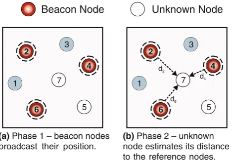
The RPE algorithm can be divided into four phases (see Fig.1). In the first phase, beacon nodes broadcast their posi-tion so they can be used as reference nodes. In the second phase, a node estimates its distance to the reference nodes by using, for example, the received signal strength indicator (RSSI) [5]. In the third phase, the node computes its position by using multilateration [5], and becomes a settled node. In the final phase, the node becomes a reference, and broadcasts its estimated position to assist its neighbors.
By using settled nodes as reference nodes, location errors are propagated. The reason is that the distance estimation process introduce errors in the estimated positions. As a con-sequence, the most distant nodes of the beacons are likely to have larger errors than the closer ones. In Fig.1, the location error for node 5 is probably greater than the location error for node 7.
The algorithm attempt to mitigate propagated errors by ignoring the worst references. The references quality is given by the residual value defined as
r esi dual(x,y)= R
i=1
(xi−x)2+(yi−y)2−di
2
(1)
Beacon Node Unknown Node Settled Node Reference Node
1
2 3
7
4
5
6
(a) Phase 1 – beacon nodes broadcast their position.
1
2 3
7
4
5
6
d4
d2
d6
(b) Phase 2 – unknown node estimates its distance to the reference nodes.
1
2 3
7
4
5
6
(c) Phase 3 – unknown node computes its posi-tion and becomes a settled node.
1
2 3
7
4
5
6
d7
d6
d4
(d)Phase 4 – The new set-tled node is used as a ref-erence.
Fig. 1 Example and phases of the recursive position estimation (RPE)
The RPE is an algorithm that uses multiple hops to deter-mine the nodes position. Hence, the network topology does not have to follow a special organization, making it suitable for outdoor scenarios.
2.1.2 Directed position estimation
The DPE [24] algorithm is similar to the RPE algorithm. The main idea of the DPE is to start the recursion at a single loca-tion, and make it follow a known direction. Then, a node can estimate its position by using only two reference neighbors and the recursion direction. This controlled recursion leads to smaller errors, compared to RPE.
To ensure that the recursion starts at a single point, the algorithm uses a fixed beacon structure. The recursion direc-tion and the beacon structure are depicted in Fig.2a. This structure has, generally, four beacons that know their dis-tance from the recursion origin and the angle between each
pair of beacons. Then, to start the recursion, these beacons inform their positions to their neighbors.
When a node receives the position from two reference neighbors (see Fig.2b), a pair of possible points results from the system: one is the correct position and the other is the incorrect. Because the direction of the recursion is known, the node can choose between the two possible solutions: the most distant point from the recursion origin is the correct choice.
The algorithm is divided into four phases. In the first phase, beacon nodes start the recursion from a single location. In the second phase, a node chooses two reference points: the pair of nodes with the largest distance between them, and closest to the recursion origin. In the third phase, the node estimates its position. This position is estimated by intersecting the two circles and choosing the most distant point from the recursion origin. In the last phase, the node becomes a reference by sending its information to its neighbors.
Fig. 2 The directed position estimation
Recursion Origin
Beacons
Unknown Nodes Recursion Direction
Reference Nodes
Y Coordinate
X Coordinate
(a)
Directed localization recursion using bea-con structure.Ref2 Ref1
Wrong Position
Recursion Direction
Right Position
Recursion Origin
The recursion direction can occasionally become wrong. To a correct estimation it is necessary to avoid two possi-ble situations: (a) when the unknown node is closer to the recursion origin than one of the two reference nodes; and (b) when both reference nodes are aligned with the recursion ori-gin. These two scenarios can be detected by comparing the distances from the possible solutions to the recursion origin with the distances from the reference nodes to the recursion origin.
The DPE also propagates localization errors, due to dis-tance estimation errors. However, propagated errors are con-siderably smaller. Oliveira et al. [24] compare the perfor-mance of the DPE with the RPE in several aspects. Their results show that the DPE outperforms RPE in many cases. The DPE works with sparse network, needs fewer beacons, and have smaller errors.
2.2 Target tracking
Target tracking algorithms aim at estimating current and future (next) location of a target. These algorithms are exposed to different sources of noise, introduced by the mea-surement process and also errors in nodes’ location that are used to estimate the target coordinates. Therefore, informa-tion fusion [20] is commonly used for filtering such noise sources. Two popular algorithms for this problem are the Kalman and Particle filters.
Several tracking solutions are based on Kalman filters (KF). The reason is that Kalman filters have been used in algorithms for source localization and tracking, especially in robotics [20]. Li et al. [16] propose a source localization algo-rithm for a system equipped with asynchronous sensors, and evaluate the performance of extended Kalman filter (EKF) [35] and unscented Kalman filter (UKF) [14] for source track-ing in non-linear systems. Olfati-Saber [23] proposes distrib-uted Kalman filtering (DKF), in which a centralized KF is decomposed into micro-KFs, so that the distributed approach has a performance equivalent to centralized KF.
Particle filters are popular for modeling non-linear sys-tems subject to non-Gaussian noise. Vercauteren et al. [32] propose a collaborative Particle Filter for jointly tracking sev-eral targets and classifying them according to their motion pattern. Arulampalam et al. [3] assess the use Particle filters and the EKF for tracking applications. Considering sensor networks, Rosencrantz et al. [26] developed a Particle Filter for distributed information fusion applied to decentralized tracking. Jiang and Ravindran [13] propose a completely dis-tributed Particle Filter for target tracking in sensor networks, where the communication cost to maintain the particles on different nodes and propagate along the target trajectory is reduced.
Souza et at. [29] assess the performance of target tracking algorithms when position information is provided by
local-ization algorithms. The authors combine the KF and PF with RPE and DPE. In this work, we combine the same algo-rithms, but we use data fusion of multiple distance estimates during the localization process to improve the target-tracking accuracy.
There are also other distributed approaches for tar-get tracking that are based on cluster [6,33,38] and tree [17,31,37] organizations for in-network data processing.
2.2.1 Kalman filter
The Kalman filter is a popular fusion method used to fuse low-level redundant data [20]. If a linear model can describe the system and the error can be modeled as a Gaussian noise, than the Kalman Filter recursively retrieves statistically opti-mal estimates.
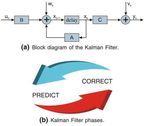
This method, as depicted in Fig. 3a, causes at each discrete-time increment a linear operator application in the current state to generate the new state. The filter considers measurement noise and, optionally, information about the controls on the system. Then, another linear operator, also subject to noise, generates the observed outputs from the true state.
The Kalman filter estimates the statexof a discrete-time
kcontrolled process that is ruled by the state-space model
xk+1=Axk+Buk+wk (2)
with measurementsyrepresented by
yk=Cxk+vk, (3)
in whichAis the state transition matrix,Bis the input control matrix that is applied to control vectoru,Cis the measure-ment matrix;wrepresent the process noise andv the mea-surement noise, where these noise sources are represented by random zero-mean Gaussian variables with covariance matricesQandRrespectively.
Based on the measurement y and the knowledge of the system parameters, the estimate of x, represented by xˆ is given by
ˆ
xk+1=(Axkˆ +Buk)+Kk(yk−Cxkˆ ), (4)
in whichKis the Kalman gain determined by
Kk=PkCT(CPkCT +R)−1, (5)
whilePis the prediction covariance matrix that can be deter-mined by
Pk+1=A(I−KkC)PkAT +Q. (6)
(a)
Block diagram of the Kalman Filter.PREDICT
CORRECT
(b)
Kalman Filter phases.Fig. 3 Kalman filter representation and phases
The measurement-update is responsible for incorporating a new measurement into the a priori estimate to obtain an improved a posteriori estimate and consists of the Eqs. (4), (5), and (6) [20]. These phases form a cycle that is maintained while the filter is fed by measurements.
Since many problems cannot be represented by lin-ear models, algorithms have emerged based on the origi-nal Kalman Filter formulation to allow these problems to be treated. The major variations of the Kalman filter for non-linear problems are the extended Kalman filter (EKF) [10] and the unscented Kalman filter (UKF) [14]. The EKF is the most popular alternative to non-linear problems. This method uses a linearized model of the process using Taylor series, because this is a sub-optimal estimator. The UKF per-forms estimations on non-linear systems without the need to linearize them, because it uses the principle that a set of dis-crete sampling points can be used to parameterize the mean and covariance. The quality of UKF estimates are close to standard KF for linear systems.
Finally, the Kalman filter model allows the elaboration of an algorithm to estimate the optimal state vector values. Thus, it is possible to generate a sequence of state values in each time unit, predicting future states using the current state, and allowing the creation of systems with real-time updates.
2.2.2 Particle filter
Particle Filters are recursive implementations of sequential Monte Carlo (SMC) methods [3]. Although the Kalman filter is a classical solution, Particle Filters represent an alternative for applications with non-Gaussian noise, especially when computational power is rather cheap and sampling rate is slow.
Unlike of the linear/Gaussian problems, the calcula-tions of the posterior distribution of non-linear/non-Gaussian problems are extremely complex. To overcome this difficulty, the Particle Filter adopts an approach called sampling impor-tance. The goal is to estimate the posterior probability den-sity, representing it as a set of particles.
This method attempts to build the posterior probability density function (PDF) based on a large number of random samples, called particles. These particles are propagated over time, sequentially combining sampling and resampling steps. At each time step, the resampling is used to discard some par-ticles, increasing the relevance of regions with high posterior probability. Each particle has an associated weight that indi-cates the particle quality. Then, the estimate is the result of the weighted sum of all particles.
The resampling step is the solution adopted to avoid the degeneration problem, where the particles have negli-gible weights after several iterations. The particles of greater weight are selected and serve as the basis for the creation of the new particles set. Furthermore, the minor particles dis-appear and do not originate descendants.
As the Kalman filter, the Particle filter algorithm has two phases: prediction and correction. In the prediction phase, each particle is modified according to the existing model, including the addition of random noise in order to simulate the effect of noise. Then, in the correction phase, the weight of each particle is reevaluated based on the latest sensory information available, so that particles with small weights are eliminated (resampling process).
3 Proposed approach
In the evaluation presented later in this work, we show that errors introduced by the localization algorithms are not suc-cessfully filtered by the tracking algorithm (Kalman and Particle filters), because the node position errors are not per-ceived as noise by the filters.
An alternative to reduce the tracking error is reducing localization errors. By reducing the localization error, we make tracking algorithms closer to their ideal operating con-ditions. Thus, we use a Kalman Filter to improve distance estimation errors and, consequently, localization and track-ing accuracy.
Ref1
Ref3
Ref2
Ref1
Ref2
Ref3 KF1
KF2
KF3 k
...
1 2...
2 1 k...
1 2 k
Fig. 4 Fusion ofkdistance estimations to improve the target tracking performance. For this task, the unknown node create a unique Kalman filter instance for each reference
In this task, the Kalman filter goal is to obtain a constant (distance) estimate. The linear system of the filter is very simple and can be configured as
xk+1=dk+1=dk+wk yk=dk+vk
(7)
in whichx andd represent the state, distance in this case, of the discrete-timek; yis a measurement value; wandv represent the process and measurement noise, respectively.
Filtering the distance estimates during localization is a simple process that ensures good results. The distance esti-mates errors are the largest contributors to overall error of the localization system, and only a small fraction of this error is generated by position computation and localization algorithm [4,24]. Some algorithms try to isolate the dis-tance estimate errors by selecting the best references based on a residual value [2], however this technique is not very efficient, because all references can cause distance estimate errors. Since the node position is calculated and used by any application, such as target tracking, it is difficult to determine the error size and direction, so the best option is to work on the error source.
4 Evaluation
In this section, we evaluate the performance of the KF and PF using the information position provided by the RPE and DPE localization algorithms. We apply the proposed approach in the localization process, where several distance estimates are used to verify its performance.
4.1 Methodology
The evaluation methodology is divided into five phases, as shown in Fig. 5. First, there is a newly deployed sensor
network with some beacon nodes, where most of the nodes do not know their position (unknown nodes), so this network must be prepared to track the target. In the second phase, a localization algorithm is applied (RPE or DPE), and during this step, several distance estimates can be used to reduce the localization errors and improve the tracking accuracy, follow-ing the proposed approach (see Sect.3). In the third phase, nodes know their position, so when three or more nodes detect the target, they compute its position with multilateration. In the fourth phase, the nodes send the target position to the sink node. In the final phase, the sink node predicts the next target position and reduces the measurement noise, performing the tracking algorithm (Kalman filter or Particle filter). While there are measurements, the target tracking continues (back to phase three).
The experiments were performed by simulation (imple-mented in Java), where the sensor field is composed of
n sensor nodes, with a communication range of rc, that are distributed in a two-dimensional squared sensor field
Q= [0,s]×[0,s]. As a proof-of-concept, we consider sym-metric communication links, i.e., for any two nodesuandv,
u reachesv if and only ifv reachesu. Thus, we represent the network by the Euclidean graph G = (V,E)with the following properties:
– V = {v1, v2, . . . , vn}is the set of sensor nodes;
– i,j ∈ Eiffvi reachesvj, i.e. the distance betweenvi
andvj is less thanrc.
To detect the target, we use the binary detection model [11,34]. In this model, for a given evente(target presence), every sensorv, whose distanced between it and the target is smaller than a detection radius rd, assuredly detects the event. Then, the probability of a sensor node to detect an event is defined as
P(v,e)=
1, ifd≤rd
0, otherwise. (8)
The default network configuration is composed of n =
150 sensors nodes randomly distributed on aQ= [0,70] ×
Fig. 5 Methodology phases: (1) a newly deployed sensor network with beacon and unknown nodes; (2) a
localization algorithm is applied, moreover several distance estimates are used to improve the tracking accuracy; (3) three or more nodes detect the target and compute its position; (4) the target position is sent to the sink node; (5) the sink node performs the tracking algorithm for predict the future target position and reduce the measurement noise, then back to phase three
1
4
3
2
5
k k+1 Unknown Nodes Beacon Nodes Settled Nodes Target Detecting Sink Node Measured Predictionarrival (TOA) and time difference of arrival (TDoA) [8,9], each range sample is disturbed by a zero-mean Gaussian vari-able with standard deviation equals to 5 % of the distance. This assumption is reasonable and leads to non-Gaussian errors in the localization algorithms [25]. During the local-ization algorithm, we vary the number of distance estimates used by the Kalman Filter as 1, 10, 20, 50, 100, and 200 measurements for each reference.
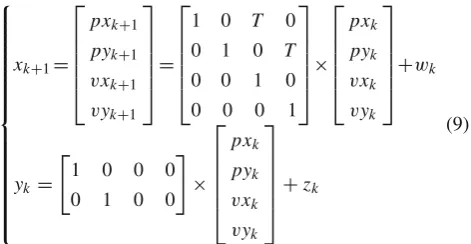
The target tracking is performed with Kalman or Parti-cle filters. The Kalman filter has its linear system equations represented by ⎧ ⎪ ⎪ ⎪ ⎪ ⎪ ⎪ ⎪ ⎪ ⎪ ⎪ ⎪ ⎪ ⎪ ⎪ ⎨ ⎪ ⎪ ⎪ ⎪ ⎪ ⎪ ⎪ ⎪ ⎪ ⎪ ⎪ ⎪ ⎪ ⎪ ⎩
xk+1=
⎡ ⎢ ⎢ ⎢ ⎢ ⎣
pxk+1
pyk+1 vxk+1 vyk+1
⎤ ⎥ ⎥ ⎥ ⎥ ⎦= ⎡ ⎢ ⎢ ⎢ ⎢ ⎣
1 0 T 0
0 1 0 T
0 0 1 0
0 0 0 1
⎤ ⎥ ⎥ ⎥ ⎥ ⎦× ⎡ ⎢ ⎢ ⎢ ⎢ ⎣ pxk pyk vxk vyk ⎤ ⎥ ⎥ ⎥ ⎥ ⎦+wk
yk =
1 0 0 0
0 1 0 0
× ⎡ ⎢ ⎢ ⎢ ⎢ ⎣ pxk pyk vxk vyk ⎤ ⎥ ⎥ ⎥ ⎥ ⎦+zk
(9)
in whichxrepresents the state of a discrete-timek, composed by the position (px,py) and velocity (vx,vy);yis a measure-ment value;wandvrepresent the process and measurement noise, respectively.
The Particle filter uses 1,000 particles. This value was set based on a previous empirical tests that showed that more than 1,000 particles do not improve tracking significantly. The Particle filter used in the experiments is represented by Algorithm1.
For illustration purposes, the Particle Filter algorithm pre-sented considers only one dimension, in whichxis the posi-tion,vis the velocity andwis the weight of eachNparticles in a discrete-timek;yis the input measurement value. First, the algorithm randomly distributes the particles (line 2). The particle propagation and the calculus of their importance con-sider the distance from each particle to the measurement posi-tion (lines 4–10). The normalizaposi-tion process (line 12) pre-pares the particles weights for the resampling process (lines 14–21). Finally, the prediction of the position is calculated (line 23).
For the sake of simplicity, we consider an uniform move-ment, so that the movement is modeled by a linear system, suitable for both Kalman and Particle filters. The target tra-jectory is composed of 1,000 points to consider a significa-tive sample. The distance between the points of the trajec-tory is 0.1 m (uniform motion) to keep the target within the area monitored. The interval between each measurement is
input : The measuredyk
output: The predictionxk+1
// Initialize the particles
1
fori=1:Ndo xi0←r andom();
2
// Sample particles from importance density and compute
3
weights
total W eight←0;
4
fori=1:Ndo
5
xki ←xki−1+vik−1+gaussi an();
6 vi
k←vik−1+gaussi an()∗0.05;
7 wi
k←1/di stance(yk,xik);
8
total W eight←total W eight+wi k;
9
end
10
// Normalize weights
11
fori=1:Ndo wi
k←wik/total W eight;
12
// Resampling
13
sli ce0
k←w0k;
14
fori=2:Ndo sli cei k ←sli ce
i−1
k +wik
15
fori=1:Ndo
16
c←r andom();
17
j←0;
18
whilej<N−1andsli cekj<cdo j← j+1;
19
r esampli ngi
k ←par ti cle j k;
20
end
21
// Result
22
fori=1:Ndo xk+1←xk+1+xi k∗wik;
23
r et ur nxk+1;
24
Algorithm 1: Particle Filter.
In Figs.6–12, each point is plotted as an average of 100 random topologies to ensure a lower variance in the results. The error bars represent the confidence interval of 99 %.
4.2 Simulation results
4.2.1 Target tracking behavior
To illustrate the behavior of the tracking algorithms, we show some snapshots in this section. In these snapshots, the RPE algorithm could not find the location of two nodes (from 150 nodes), and the average error of the node locations is 3.49 m. Adopting the same instance, the DPE algorithm managed to estimate the location of every node, and the average location error is 2.56 m.
These two scenarios are compared with the ideal setting, in which the localization system is perfect. For all cases, the performance of Kalman and Particle filters are presented. The results are summarized in Table1.
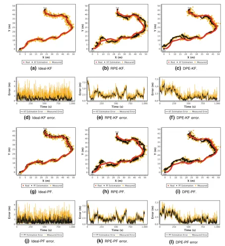
The Fig.6a–c shows a target moving through the sensor field (red line). Orange points represent measurements and blue points are the results of Kalman Filter tracking algo-rithm. Figure6d–f shows the error calculated from real target and Kalman Filter estimation for each measured point. Figure 6g–l represents the same case using the Particle Filter track-ing algorithm instead. These figures illustrates the influence
of the localization errors caused by each algorithm. In gen-eral, the greater the localization error, the greater the tracking error, independent of the tracking algorithm. The influence of localization errors is clearly visible in the region around point (20, 15) in Fig.6c, in which localization errors lead to a wrong track estimation.
Tracking with Kalman Filter has better results when node’s location information are ideal, or when they are esti-mated by the DPE. However, when the node locations are estimated by the RPE, the Particle Filter presents the best results. The reason is that the Particle Filter is less affected by measurement errors, this fact becomes clear in the follow-ing sections.
As a general conclusion, Fig. 6 shows that both filters successfully reduce the errors resulting from the estimation of the target location, but errors resulting from the localization algorithms are not significantly filtered.
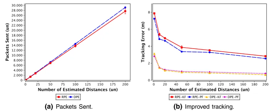
4.2.2 Costs and benefits of multiple distance estimates.
More distance estimates during the localization process can reduce the localization and tracking errors. However, it is necessary to send additional packets, i.e., more resources will be consumed to get this benefit. Therefore, in this section we evaluate the costs and benefits of using several distance esti-mates. This analysis is important, since it helps define how much you should spend for a given performance in the target tracking.
Both the RPE and DPE have the communication com-plexity ofO(n), wherenis the number of nodes. The Fig.7a shows the number of packets sent when the number of dis-tance estimates increases. Usingkdistance estimates causes each beacon and settled node to broadcast its positionktimes, increasing the communication complexity to O(kn). This figure also shows that the RPE sends fewer packets than the DPE. This occurs because of the network density used in the experiment that lead RPE, in some topologies, to esti-mate fewer node positions than DPE, so these nodes do not broadcast their location information, reducing the number of packets sent.
The Fig.7b shows the improvement in accuracy of track-ing when the number of distance estimates increase. Ustrack-ing 10 distance estimates already provides a significant improve-ment when compared to results obtained with only 1 esti-mation. In the target tracking using the RPE, the Particle Filter has better results, because this algorithm reduces a small fraction of non-Gaussian noise introduced by local-ization algorithm. In target tracking with DPE, the Kalman Filter becomes more accurate with more than 10 distance estimates, because the localization error is pretty low, so that the Kalman Filter starts to operate under ideal conditions.
(a)Ideal-KF (b)RPE-KF. (c) DPE-KF.
(d)Ideal-KF error. (e) RPE-KF error. (f) DPE-KF error.
(g) Ideal-PF. (h) RPE-PF. (i) DPE-PF.
(j) Ideal-PF error. (k) RPE-PF error. (l) DPE-PF error
Fig. 6 Performance of Kalman and Particle filters using the RPE and DPE localization algorithms
comparison with the required cost. Using 10 distance esti-mates is enough to achieve improvements of 50 % with a reasonable cost. Until 50 distance estimates can significantly reduce the tracking error, but most estimates (100 and 200) lead to a little improvement of results with high cost.
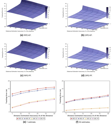
4.2.3 Impact of distance estimation inaccuracy
Distances estimated by sensor nodes are not perfect. Depend-ing on the monitored environment, the associated errors can
be greater, which affects the tracking performance. In gen-eral, these errors can be modeled by a zero-mean Gaussian variable, in which the standard deviation is a percentage of the actual distance [4].
(a)
Packets Sent.(b)
Improved tracking.Fig. 7 Costs and benefits of multiple distance estimates
have errors smaller than 1 m. While larger deviations repre-sent errors obtained by more imprecise methods, like RSSI. Figure8a–d presents the error performance by varying the distance estimation inaccuracy and the number of estimates, showing 3D graphs with the combination of RPE and DPE with KF and PF. Figure8e, f shows the cases of 1 and 50 distances estimates, respectively.
When the distance estimation inaccuracy is low (between 5 and 10 % of the distance), the accuracy improvement of the target tracking using DPE is negligible, regardless of the number of distance estimates used. When this imprecision is high (between 15 and 30 %), with 50 distances estimates or more, note that the average error converges to 1 m (Fig.8b, d). However, with RPE, the improvement is notice-able even when the distance estimates inaccuracy is low (Fig.8a, c).
It is also interesting to note in Fig.8e, f that the Particle filter outperforms the Kalman Filter, especially when RPE is chosen as the localization algorithm. The reason is that the non-linearity and non-Gaussian nature of the Particle Filter results in reducing a small fraction of the non-Gaussian noise introduced by the localization algorithm.
4.2.4 Impact of the network density
The impact of the density of the network is evaluated by increasing the number of nodes in the same sensor field, so that the network density varies from 0.03 to 0.07 nodes/m2. The smallest density used in this experiment allows both the RPE and DPE algorithms to estimate the location of the most of the sensor nodes.
In this case, Fig.9 shows that, for the DPE algorithm, the target tracking error remains constant independent of the network density. The reason is that the same beacon structure is used regardless the network density. However, for the RPE
algorithm, the number of beacons increase with the network density, because we ensure that 5 % of the nodes are beacons. As a result of the increasing number of beacons, the tracking error reduces accordingly.
Multiple distance estimates are important for improving the target tracking accuracy when the RPE is used, especially in sparse networks, as show in Fig.9a and c. With the DPE instead, the network density does not interfere in the target tracking error. Therefore, for 50 distance estimates or more the average error converges to 0.7m (Fig.9b, d).
Figures9(e and f) show that with a single distance esti-mate during the location process, the Particle Filter is slightly better with both RPE and DPE. The reason is that it filters a small fraction of the non-Gaussian localization errors. When we use 50 distance estimates, the performance of the Kalman Filter becomes equivalent to the Particle Filter in the case of RPE and better in the case of DPE, since the Kalman Filter operates under ideal conditions with low localization errors.
4.2.5 The impact of the network scale
In this section, we evaluate how the network scale affects the combinations of localization and tracking algorithms.
In this context, we vary the number nodes from 100 to 350, while keeping a constant density of 0.03 nodes/m2. There-fore, the monitored area is resized according to the number of sensor nodes. As the percentage of beacons used by RPE is 5 %, the number of beacons also increases according to the number of nodes in this case. The DPE keeps using only a single structure of four beacons.
5 10 15 20 25 30
1 50 100
200 0
3 6 9 12 15 18
Distances Estimation Inaccuracy (% of the distance)
Estimates (un)
Tracking Error (m)
0 3 6 9 12 15 18
(a) RPE-KF.
5 10 15 20 25 30
1 50 100
200 0
3 6 9 12 15 18
Distances Estimation Inaccuracy (% of the distance)
Estimates (un)
Tracking Error (m) 0 3
6 9 12 15 18
(b) DPE-KF.
5 10 15 20 25 30
1 50 100
200 0
3 6 9 12 15 18
Distances Estimation Inaccuracy (% of the distance)
Estimates (un)
Tracking Error (m) 0 3
6 9 12 15 18
(c) RPE-PF.
5 10 15 20 25 30
1 50 100
200 0
3 6 9 12 15 18
Distances Estimation Inaccuracy (% of the distance)
Estimates (un)
Tracking Error (m) 0 3
6 9 12 15 18
(d) DPE-PF.
(e) 1 estimate. (f) 50 estimates.
Fig. 8 Impact of distance estimation inaccuracy
with the RPE, the tracking errors remains almost constant, because the number of beacons increase with the network scale (cf. [24]).
When there are many nodes in network (between 250 and 350), using multiple distance estimates in DPE improves sig-nificantly the target tracking accuracy, however they have lit-tle influence when there are few nodes (Fig.10b, d). With RPE instead, the usage of multiple distance estimates is important for any number of nodes (Fig.10a, c).
4.2.6 The impact of the number of beacons
0.03 0.04 0.05 0.06 0.07
1 50 100
200 0
2 4 6 8 10 12 14
Density (nodes/m2)
Estimates (un)
Tracking Error (m) 0 2
4 6 8 10 12 14
(a) RPE-KF.
0.03 0.04 0.05 0.06 0.07
1 50 100
200 0
2 4 6 8 10 12 14
Density (nodes/m2)
Estimates (un)
Tracking Error (m) 0 2
4 6 8 10 12 14
(b) DPE-KF.
0.03 0.04 0.05 0.06 0.07
1 50 100
200 0
2 4 6 8 10 12 14
Density (nodes/m2)
Estimates (un)
Tracking Error (m) 0 2
4 6 8 10 12 14
(c) RPE-PF.
0.03 0.04 0.05 0.06 0.07
1 50 100
200 0
2 4 6 8 10 12 14
Density (nodes/m2)
Estimates (un)
Tracking Error (m) 0 2
4 6 8 10 12 14
(d) DPE-PF.
(e) 1 estimate. (f) 50 estimates.
Fig. 9 Impact of the network density
In this experiment, the number of beacons is increased from 5 to 35 % of the total number nodes. A greater number of beacons means that the localization algorithm has more references for estimating the location of remaining nodes, which leads to smaller errors. Hence, the tracking error is also inversely proportional to the number of beacons. This behavior is depicted in Fig.11.
When the amount of beacon nodes is significantly large, the localization error becomes so small that the Kalman Fil-ter tends to have betFil-ter results than the Particle FilFil-ter, it is up
100 150 200 250 300 350
1 50 100
200 0
3 6 9 12 15
Number of Nodes (un)
Estimates (un)
Tracking Error (m) 0
3 6 9 12 15
100 150 200 250 300 350
1 50 100
200 0
3 6 9 12 15
Number of Nodes (un)
Estimates (un)
Tracking Error (m) 0
3 6 9 12 15
100 150 200 250 300 350
1 50 100
200 0
3 6 9 12 15
Number of Nodes (un)
Estimates (un)
Tracking Error (m)
0 3 6 9 12 15
100 150 200 250 300 350
1 50 100
200 0
3 6 9 12 15
Number of Nodes (un)
Estimates (un)
Tracking Error (m)
0 3 6 9 12 15
(a) RPE-KF. (b) DPE-KF.
(c) RPE-PF. (d)DPE-PF.
(e) 1 estimate. (f) 50 estimates.
Fig. 10 Tracking scale
4.2.7 The impact of the beacon structure
As stated earlier, increasing numbers beacons by structure in the DPE does not improve the localization results. However, the DPE may benefit from multiple beacon structures [24]. Thus, to evaluate the performance of the target tracking algo-rithms with multiple beacon structures, we vary the number of such structures from 1 to 5. This experiment represents a situation for the DPE algorithm that is analogous to the previous experiment for the RPE algorithm.
5 10 15 20 25 30 35
1 50 100
200 0
5 10 15 20
Beacons (%)
Estimates (un)
Tracking Error (m)
0 5 10 15 20
5 10 15 20 25 30 35
1 50 100 200 0
5 10 15 20
Beacons (%)
Estimates (un)
Tracking Error (m)
0 5 10 15 20
(a)
RPE-KF.(b)
RPE-PF.(c)
1 estimate.(d)
50 estimates.Fig. 11 Impact of the number of beacons
error converges to 0.6 m regardless of the number of beacon structures available (Fig.12a, b).
5 Conclusions and future work
In this work, we demonstrated how information fusion can reduce errors during the localization process, while assessing the impact of actual localization algorithms on target tracking algorithms. For these evaluations, we chose the RPE and DPE algorithms to compute node positions, since RPE is a pioneer solution and DPE is more accurate and cheaper than the RPE. The target tracking techniques we have chosen were the Kalman and Particle filters. These filters are very popular and can be considered as canonical solutions for the target tracking problem.
As a general conclusion, by using up to 50 distance esti-mates ensures better results in the target tracking with a moderate cost. Above this value, the errors converges, so the reduction of errors is small compared to the associated cost. Furthermore, the reduction in localization error using
information fusion enhances the performance of Kalman Fil-ter over the Particle FilFil-ter, especially when the DPE is used. Kalman and Particle filters successfully filter the errors associated with the target location estimation. However, the errors introduced by the localization algorithms are not suc-cessfully filtered by the tracking algorithm. The reason is that the Kalman Filter is not designed to filter non-Gaussian noise. On the other hand, the Particle Filter is designed to filter non-Gaussian noise. Consequently, the Particle Filter tends to outperform the Kalman as the localization errors increase. However, even the Particle Filter cannot significantly filter the non-Gaussian localization errors. Results show that for tracking applications with severe accuracy constraints, the localization algorithms need to improve their estimations to guarantee the performance of target tracking algorithms.
1 2 3 4 5
1 50 100
200 0
1 2 3 4
Beacon Structures (un)
Estimates (un)
Tracking Error (m)
0 1 2 3 4
1 2 3 4 5
1
50
100
200 0
1 2 3 4
Beacon Structures (un)
Estimates
Tracking Error (m)
0 1 2 3 4
(a)
DPE-KF.(b)
DPE-PF.(c)
1 estimate.(d)
50 estimates.Fig. 12 Impact of the beacon structure
Table 1 Target tracking errors
Localization algorithm Tracking error (m)
KF PF
RPE 2.39 2.32
DPE 1.87 1.94
Ideal 0.43 0.61
tracking algorithms that use such information to compensate and reduce the impact of localization errors, depending of the localization algorithm used.
Another future direction includes reducing the location algorithms inaccuracy by using all the location information reported to nodes. These algorithms usually provide a min-imum number of references (three for the RPE and two for the DPE) required for calculating the node position, ignoring the additional information received after the calculation. This approach can lead to accuracy improvement, and it does not
require extra communication. Finally, the cross-layer design of localization and tracking algorithms, not explored yet, may lead to improved solutions for both problems.
Acknowledgments This work is supported by the Brazilian Nat-ional Council for Scientific and Technological Development (CNPq), under the grant numbers 474194/2007-8 (RastroAM), 55.4087/2006-5 (SAUIM) and 575808/2008-0 (Revelar), and also the the Amazon State Research Foundation (FAPEAM), trough the grant 2210.UNI175.3532. 03022011 (Projeto Anura—PRONEX 023/2009).
References
1. Akyildiz IF, Su W, Sankarasubramaniam Y, Cayirci E (2002) Wire-less sensor Networks: a survey. Comput Netw 38:393–422 2. Albowicz J, Chen A, Zhang L (2001) Recursive position
estima-tion in sensor networks. In: Proceedings of the 9th internaestima-tional conference on network protocols (ICNP’01), pp 35–41
4. Bachrach J, Eames AM, Eames AM (2005) Localization in sensor networks, chapter 9, pp 277–310. Wiley, New York
5. Boukerche A, de Oliveira HABF, Nakamura EF, Loureiro AAF (2007) Localization systems for wireless sensor networks. IEEE Wireless Commun 14:6–12
6. Chong CY, Zhao F, Mori S, Kumar S (2003) Distributed tracking in wireless ad hoc sensor networks. In: Proceedings of the 6th interna-tional conference of information fusion (Fusion’03), pp 431–438 7. Ehsan S, Bradford K, Brugger M, Hamdaoui B, Kovchegov Y,
Johnson D, Louhaichi M (2012) Design and analysis of delay-tolerant sensor networks for monitoring and tracking free-roaming animals. Trans Wireless Commun 11(3):1220–1227
8. Fukuda K, Okamoto E (2012) Performance improvement of TOA localization using IMR-based NLOS detection in sensor networks. In: Proceedings of the 26th international conference on information networking (ICOIN’12), pp 13–18
9. Gibson JD (1999) The mobile communication handbook. IEEE Press, New York
10. Grewal MS, Andrews AP (2001) Kalman filtering: theory and prac-tice using MATLAB. Wiley, New York
11. He T, Bisdikian C, Kaplan L, Wei W, Towsley D (2010) Multi-target tracking using proximity sensors. In: Proceedings of the military communications conference (MILCOM’10), San Jose, California, USA, pp 1777–1782
12. He T, Huang C, Blum BM, Stankovic JA, Abdelzaher T (2003) Range-free localization schemes for large scale sensor networks. In: Proceedings of the 9th ACM international conference on mobile computing and networking (MobiCom’03), pp 81–95
13. Jiang B, Ravindran B (2011) Completely distributed particle filters for target tracking in sensor networks. In: Proceedings of the 25th parallel distributed processing, Symposium (IPDPS’11)
14. Julier SJ, Uhlmann JK (1997) A new extension of the kalman filter to nonlinear systems. In: Proceedings of the international aerosense, Symposium (SPIE’97), pp 182–193
15. Kalman RE (1960) A new approach to linear filtering and prediction problems. J Basic Eng 82:35–45
16. Li T, Ekpenyong A, Huang YF (2006) Source localization and tracking using distributed asynchronous sensor. IEEE Trans Signal Process 54:3991–4003
17. Lin CY, Peng WC, Tseng YC (2006) Efficient in-network moving object tracking in wireless sensor networks. IEEE Trans Mobile Comput 5:1044–1056
18. Lin KW, Hsieh MH, Tseng VS (2010) A novel prediction-based strategy for object tracking in sensor networks by mining seamless temporal movement patterns. Expert Syst Appl 37:2799–2807 19. Mazomenos EB, Reeve JS, White NM (2009) A range-only
tracking algorithm for wireless sensor networks. In: International conference on advanced information networking and applications workshops (AINAW’07), pp 775–780
20. Nakamura EF, Loureiro AAF, Orgambide ACF (2007) Information fusion for wireless sensor networks: methods, models, and classi-fications. ACM Comput Surv 39:1–55
21. Neto JMRS, Silva JJC, Cavalcanti TCM, Rodrigues DP, da Rocha Neto JS, Glover IA (2010) Propagation measurements and model-ing for monitormodel-ing and trackmodel-ing in animal husbandry applications. In: Proceedings of the instrumentation and measurement technol-ogy conference (I2MTC’10). Austin, Texas, USA, pp 1181–1185 22. Niculescu D, Nath B (2001) Ad hoc positioning system (aps). In: Proceedings of the global telecommunications conference GLOBECOM’01), pp 2926–2931
23. Olfati-Saber, R.: Distributed kalman filter with embedded con-sensus filters. In: Proceedings of the 44th Conference on Deci-sion and Control—European Control Conference (CDC-ECC’05), pp. 8179–8184 (2005)
24. Oliveira HABF, Boukerche A, Nakamura EF, Loureiro AAF (2009) An efficient directed localization recursion protocol for wireless sensor networks. IEEE Transactions Computing 58:677–691 25. Oliveira, H.A.B.F., Nakamura, E.F., Loureiro, A.A.F., Boukerche,
A.: Error analysis of localization systems in sensor networks. In: Proceedings of the 13th International Symposium on Geo-graphic, Information Systems (GIS’05), pp. 71–78 (2005) 26. Rosencrantz M, Gordon G, Thrun S (2003) Decentralized sensor
fusion with distributed particle filters. In: Proceedings of the Con-ference on Uncertainty in AI (UAI)
27. Sichitiu, M.L., Ramadurai, V.: Localization of wireless sensor net-works with a mobile beacon. In: Proceedings of the International Conference on Mobile Ad-hoc and Sensor Systems (MASS’04), pp. 174–183 (2004)
28. Souza, E.L., Campos, A., Nakamura, E.F.: Tracking targets in quan-tized areas with wireless sensor networks. In: Proceedings of the 36th Local Computer Networks (LCN’11), pp. 235–238. Bonn, Germany (2011)
29. Souza, E.L., Nakamura, E.F., de Oliveira, H.A.: On the perfor-mance of target tracking algorithms using actual localization sys-tems for wireless sensor networks. In: Proceedings of the 12th ACM international conference on Modeling, analysis and simula-tion of wireless and mobile systems (MSWiM ’09), pp. 418–423. Tenerife, Canary Islands, Spain (2009)
30. Tatham, B., Kunz, T.: Anchor node placement for localization in wireless sensor networks. In: Proceedings of the 7th Conference on Wireless and Mobile Computing, Networking and, Communi-cations (WiMob’11), pp. 180–187 (2011)
31. Tsai HW, Chu CP, Chen TS (2007) Mobile object tracking in wire-less sensor networks. Computer Communications 30:1811–1825 32. Vercauteren T, Guo D, Wang X (2005) Joint multiple target tracking
and classification in collaborative sensor networks. IEEE Journal on Selected Areas in Communications 23:714–723
33. Walchli, M., Skoczylas, P., Meer, M., Braun, T.: Distributed event localization and tracking with wireless sensors. In: Proceedings of the 5th International Conference on Wired/Wireless Internet, Communications (WWIC’07), pp. 247–258 (2007)
34. Wang Z, Bulut E, Szymanski BK (2010) Distributed energy-efficient target tracking with binary sensor networks. ACM Trans-actions on Sensor Networks 6(4):1–32
35. Welch, G., Bishop, G.: An introduction to the kalman filter. In: The 28th International Conference on Computer Graphics and Interac-tive, Techniques (SIGGRAPH’01) (2006)
36. Yang, H., Sikdar, B.: A protocol for tracking mobile targets using sensor networks. In: Proceedings of the 1st International Work-shop on Sensor Network Protocols and Applications (SNPA’03), pp. 71–81 (2003)
37. Zhang W, Cao G (2004) Dctc: Dynamic convoy tree-based collab-oration for target tracking in sensor networks. IEEE Transactions on Wireless Communications 3:1689–1701