DOI 10.1007/s13173-010-0026-y O R I G I N A L PA P E R
Structured Markovian models for discrete spatial mobile node
distribution
Fernando Luís Dotti·Paulo Fernandes· Cristina M. Nunes
Received: 10 June 2010 / Accepted: 2 December 2010 / Published online: 12 January 2011 © The Brazilian Computer Society 2011
Abstract The study and characterization of node mobility in wireless networks is extremely important to foresee the node distribution in the network, enabling the creation of suitable models, and thus a more accurate prediction of per-formance and dependability levels.
In this paper we adopt a structured Markovian formalism, namely SAN (Stochastic Automata Networks), to model and analyze two popular mobility models for wireless networks: the Random Waypoint and Random Direction.
Our modeling considers mobility over a discrete space, i.e., over a space divided in a given number of slots, allowing a suitable analytical representation of structured regions. We represent several important aspects of mobility models, such as varying speed and pause times, and several border behav-iors that may take place. One, two, and three-dimensional models are presented. For the two-dimensional models, we show that any regular or irregular convex polygon can be modeled, and we describe several routing strategies in two dimensions.
In all cases, the spatial node distribution obtained from the steady state analysis is presented and whenever analo-gous results over continuous spaces were available in the lit-erature, the comparison with the ones obtained in this paper is shown to be coherent.
The order of authors is merely alphabetical. Paulo Fernandes and Fernando Luís Dotti are partially funded by CNPq, Brazil. F. Luís Dotti·P. Fernandes (
)·C.M. NunesFACIN–PUCRS, Av. Ipiranga, 6681, Porto Alegre, Brazil e-mail:[email protected]
F. Luís Dotti
e-mail:[email protected] C.M. Nunes
e-mail:[email protected]
Besides showing the suitability of SAN to model this kind of reality, the paper also contributes to new findings for the modeled mobility models over a noncontinuous space.
Keywords Structured stochastic modeling formalisms· Mobile nodes·Markovian models
1 Introduction
Mobility keeps gaining in importance, playing a significant role in the design and implementation of communications infrastructures and distributed systems. The study of mobil-ity in a broad spectrum has impacted a wide range of tech-nical results such as new process calculi [40], new distrib-uted programming paradigms [23], and a large set of new and revisited distributed algorithms and protocols, such as reported in [1,4,39,45] to mention a few.
Methods for the representation and analysis of distributed systems are important since such systems are often too ex-pensive to prototype and nontrivial to monitor aspects that become more challenging when mobility is involved; espe-cially, the quantitative analysis of mobile systems becomes of paramount importance. Very often the properties of mo-bile systems can only be considered in a quantitative way due to the several aspects involved and wide possibility of behavior. The study and characterization of mobility models is very important in order to analyze a given distributed sys-tem where mobility is present in one of the possible forms.
One of the cases rarely considered is the spatial distrib-ution when the nodes move over a discrete space. Such sit-uation may occur when nodes move on a grid like a net of corridors in a building or streets in a city. An even clear sit-uation of discrete space are coarser models, where the exact position is not needed, but the identification of a room or access point in use is the relevant information.
It is not a coincidence that such cases of mobility are not usually modeled, since either their mathematical formula-tion becomes quite complex or state based models for these realities easily become intractable due to the huge number of possible states, i.e., the well-known state space explosion problem. In fact, other initiatives to model similar realities, e.g., street movement [14,48] does not tackle discrete space, but rather consider a set of continuous lines.
On the other side, structured formalisms such as Sto-chastic Petri Nets [2], Stochastic Process Algebra [27], and Stochastic Automata Networks—SAN [44] are inherently discrete state and provide powerful concepts to stepwise build detailed mobility models. Probably the greatest ad-vantage of using structured formalisms is the possibility to perform numerical solutions rather than simulation experi-ments. Numerical solutions deliver exact probabilities that does not suffer from the accuracy and statistical relevance issues common to simulation approaches [17].
Actually, the numerical analysis literature [12,18,19,
33] acknowledges the computational benefits to use struc-tured representations in analytical modeling and numerical solution. Therefore, we consider that the discussion of the suitability of such methods to describe and solve mobility models is important. Among the options of structured for-malisms, we have chosen SAN basically due to the authors previous experience. To our experience, the use of other above mentioned formalisms would lead to analogous dis-cussions and results.
In this paper, we focus on the analysis of mobility models typically employed in wireless network, more specifically we model and analyze two mobility models: Random Way-point and Random Direction. The Random WayWay-point mobil-ity model [5] is one of the most used in wireless networks re-search [7,8,11,28,32,38]. The Random Direction [47] was also chosen since it is considered an approximation of real movement behavior for several classes of applications and, therefore, often used [5,21,26, 43,51]. The main objec-tive of this analysis is to derive the spatial node distribution which affects directly the performance and dependability of the used protocols [34,43]. In this context, our contribution is the following:
• We introduce the use of SAN formalism and show that this method lends itself to the formalization of mobility models, providing explicit and non-ambiguous descrip-tion of such models. Besides, the structured nature intrin-sic of the SAN formalism allows to stepwise enrich the
description level of detail when compared to continuous-state models.
• We formally describe the Random Waypoint mobility model in SAN and show the compatibility of our results with existing continuous state space studies for square ar-eas. Further, we extend the analytical model of the Ran-dom Waypoint to analyze the impact of representing more detailed aspects, namely apausetime while the mobile nodes do not move and the choice of different routing strategies. Note that such analysis of routing strategies is only meaningful due to the use of a discrete state space modeling adopted.
• We show the ability to model any surface in the shape of regular or irregular convex polygons. The modeling of such surfaces was carried out considering the Random Waypoint mobility model. Additionally, the resulting spa-tial node distributions for surfaces in the shape of some regular polygons, such as hexagon and triangle, are co-herent with those found in the literature considering con-tinuous spatial distribution.
• We formally describe the Random Direction mobility model using SAN and we show the results achieved with the spatial node distribution. For instance, we show that the pause does not affect the spatial node distribution probability in the one and two dimensional cases. An analysis of nonsquare surfaces is not represented in this paper, but it can be developed analogously to the pre-sented for Random Waypoint models.
It is important to point out that it is not the goal of this paper to defend the use of Random Waypoint and Random Direction as valid models for describing human mobility, or any other particular behavior. For those issues, the interested reader may find extensive and relevant material in [24,30,
37]. The choice of modeling RWP and RD is based on the abundance of discussion and results for these mobility mod-els in the area.
2 Mobility models
The literature presents many studies classifying different mobility models for wireless networks [5,13, 31]. These models are used to represent the movement of mobile nodes in a wireless network, and they can be split in individual and group models. The individual mobility models represent the independent movement behavior of one mobile node, while the group mobility models are used when a group of nodes have a common behavior in the choice of their movements. The modeling of individual mobility is simpler to imple-ment, because the node movement can be done through in-dependent events. Due to this characteristic, the individual models are the most used to evaluate wireless networks, as in [3,6,7,31]. The quantitative analysis of such models di-rectly influences the estimation of performance and depend-ability levels of wireless networks.
As mentioned in the previous section, in this work, we focus on the individual mobility models Random Waypoint and Random Direction, which are discussed below.
2.1 Random waypoint mobility model
In the Random Waypoint Mobility model [7,13], the mo-bile node randomly chooses a destination and moves to this destination with constant speed. When reaching the desti-nation, the mobile node remains stopped for some time and then begins the whole process all over again with the same rules. This model and its variations are widely used. Some examples of its use can be found in [7,8,11,28,29,32,38,
42,46].
Several authors consider the Random Waypoint to ob-tain the spatial node distribution, allowing one to derive im-portant performance and dependability parameters. Studies about node connectivity using Random Waypoint as mobil-ity model can be found in [15,29,36,49].
Royer et al. [47] carry out an analysis by simulation on the spatial node distribution for the Random Waypoint. In [47], it was noticed a higher probability of the node be-ing in the center of the simulated area. A detailed analyti-cal study of spatial node distribution generated by the Ran-dom Waypoint mobility model was presented by Bettstetter in [7]. The results achieved there were also validated by sim-ulation studies for one- (line) and two-dimensional (square) models without pause time.
Resta and Santi in [46] generalize the analysis of [7] al-lowing pause time and speed to be changed. They derive an explicit formula of the one-dimensional spatial node distrib-ution, and an approximated formula for the two-dimensional case.
Hyytiä et al.in [29] derive an explicit expression for the spatial node distribution of Random Waypoint in convex domains and they also demonstrate the use of the result
for various shapes of the domain. They derive an polyno-mial approximation for density function for regular trian-gles, squares, and hexagons, comparing some of their results with [7]. Besides, they analyze Random Waypoint models and some applications, such as connectivity and traffic load in ad hoc networks.
The studies have shown that although the initial node po-sitioning is taken from an uniform random distribution, the mobility model changes this distribution during the move-ment. This effect occurs because nodes tend to cross the center of the modeled region with a relatively high fre-quency and, without a pause time, the choices are inde-pendent of the node speed. However, as the pause time in-creases, the node distribution approximates the uniform dis-tribution.
The Random Waypoint mobility model is also used in others contexts. Jayakumar et al. [32] and Kumar et al. [35] used Random Waypoint to evaluate routing protocols to MANET (Mobile Ad hoc Network). Besides, a study in the context of cellular networks is presented by Hyytiä et al. in [28].
2.2 Random direction mobility model
The Random Direction is another mobility model used to analyze and simulate the movement of mobile nodes in a wireless network. Different from the Random Waypoint, the choice of new destination is done through a new direc-tion, a speed to travel, and a time duration for this travel [25,41].
One important aspect of the Random Direction mobility model is the possible behavior when reaching the border of the area considered, i.e., the border behavior. In [5], Bettstet-ter shows three different border rules:Bounce, Delete and Replace,and Wrap Around. These border rules guarantee that the number of nodes remains constant during the analy-sis. In theBounceborder rule, when the node achieves the border, it reflects back to the simulation area. The new angle is chosen according to the previous angle with the reached border [26,47]. In theDelete and Replace, according to [5], the node is deleted and a new node is created on a randomly chosen point in the simulation area. In theWrap Around, the node continues the movement and reenters in the opposite border with the same speed and direction parameters. This approach models a torus shape surface [22].
node chooses another direction between 0 and 180 degrees and continues the process.
In the basic model considered by Royer et al. [47], the mobile node randomly selects a direction and a destina-tion along this traveling direcdestina-tion, thus it is not forced to travel until the border. Besides, a speed is also randomly chosen. Once it reaches the destination, it remains station-ary for some predefined pause time. At the end of the pause time, the process is repeated. If a border of the simulation area is reached, it reflects back into simulation area, using theBounceborder rule. Some results with simulations about traffic load and node density using this model are presented in [47] and [43].
In [5], with the aim of providing a better of mobility be-havior to real mobility bebe-havior, Bettstetter employs a com-bination of principles for direction and speed control that makes the movement of users smoother. A new destination is chosen by choosing a new direction. The speed and direction changes are both probabilistic. Two stochastic processes are used: one process determines at what time a mobile station changes its speed, and the other process determines when the direction is changed. The speed is changed incrementally by the current acceleration of the mobile node, and also the di-rection change is smooth: the didi-rection is changed in several steps until the new target direction is achieved. Besides, the author analyzes the spatial node distribution using Random Direction as mobility model and modifying the rate in which the speed and the direction changes. The border behavior used wasDelete and Replace, since the others presented an uniform spatial node distribution. Our approach in Sect.5is similar to the principles adopted in [5].
Further work on the Random Direction model is also pre-sented in Di et al. [21], where a mathematical model of a 3D space is proposed and compared to simulation results. Analogously to the Random Waypoint, the Random Direc-tion model is used in he evaluaDirec-tion of MANET routing pro-tocols such as Ad-hoc On-Demand Distance Vector Routing (AODV), Destination Sequenced Distance Vector (DSDV), Dynamic Source Routing (DSR) and Temporally-Ordered Routing Algorithm (TORA) [35].
3 SAN—stochastic automata networks
The SAN formalism was proposed by Plateau [44] and its basic idea is to represent a whole system by a collection of subsystems with an independent behavior (local transitions) and occasional interdependencies (functional ratesand syn-chronizing events). Each subsystem is described as a sto-chastic automaton, i.e., an automaton in which the transi-tions are labeled with probabilistic and timing information. Hence, one can build a continuous-time stochastic process related to a SAN model, i.e., a SAN model has an equiva-lent Markov chain model [9,50].
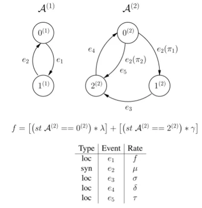
Fig. 1 Example of a SAN model
There are two types of events that change the state of a SAN model:local events andsynchronizing events. Local events change the model state changing the state of only one automaton. Synchronizing events, in opposition, can change simultaneously the states of more than one automa-ton.
The other possibility of interaction among automata is the use of functional rates. Any event occurrence rate may be expressed by a constant value inR+(a positive real number) or by a function of the state of other automata intoR+∪ {0}. In opposition to synchronizing events, functional rates are one-way interaction among automata, since it affects only the automaton where it appears and not the automata from which it depends. Figure1presents a SAN model with two automata, one synchronizing (e2) and four local events (e1, e3,e4ande5).
In this example, the rate of the evente1is not a constant rate, but a functional ratef described with the SAN nota-tion1employed by the PEPS software tool [10]. The inter-pretation off defines the firing of the transition from state 0(1) to 1(1)with rateλif automatonA(2)is in state 0(2), or rateγif automatonA(2)is in state 2(2). If automatonA(2)is in state 1(2), the transition from state 0(1)to 1(1)does not oc-cur (rate equal to zero). It is important to observe that the use of functions allows a compact and flexible way to describe in one single (local or synchronizing) event alternative be-haviors [9].
Another important point to observe in this example is the evente2, where two alternative occurrences exists for
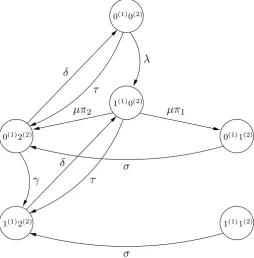
Fig. 2 Equivalent Markov chain
tomatonA(2). The occurrence of evente2could then change the state of automatonA(1)from 1(1)to 0(1)at the same time when the automatonA(2)changes from state 0(2)to alterna-tively 1(2) (with probabilityπ1) or to 2(2) (with probabil-ityπ2). Actually, every time a local or synchronizing event may change a local state to two or more other states a prob-ability of choice must be defined.
Figure 2 shows the equivalent Markov chain model to the presented SAN model. Assuming the state 0(1)0(2) as an initial state, only five of the six states in this model are reachable. To deal with such models, it is usual to express either: an initial state and let the reachable state space be computed by possible firing sequences; or a function within the product state space returning a nonzero value for reach-able global states.
For the model in Fig. 1, the reachability function must exclude the global state 1(1)1(2), thus:
Reachability=!stA(1)==1(1)&&stA(2)==1(2) Roughly, we can say that a SAN model complexity to compute a stationary or transient solution is usually propor-tional to the size of its product state space, i.e., the number of possible combinations of local (automata) states. However, according to the solution method chosen, this can vary con-siderably. Nevertheless, from an efficiency general perspec-tive it is almost always interesting to obtain a SAN model with minimum product state space, i.e., a model with the smaller number of automata, each one of them with as few local states as possible.
4 Random waypoint
Within this section, we discuss one and two-dimensional SAN models for the Random Waypoint mobility. Part of these results were presented in [20] where only linear (1D) and square (2D) areas were considered. In this section, we show these previous results and extend to consider 2D areas that can be any convex (even irregular) polygons.
4.1 Random waypoint 1D SAN model
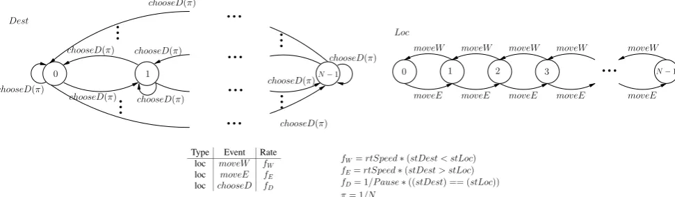
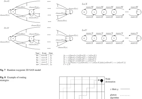
In the one-dimensional case, we define a SAN model to rep-resent a region ofMmeters modeled as a line withN slots, where one node can move to the east or to the west. Model such reality using a discrete space formalism is quite intu-itive. The observations fulfilled the expectations in the sense that the greater the N, the more the results are similar to those found in the literature for continuous space situations. Figure3 describes a SAN model composed of two au-tomata, calledDestandLoc. AutomatonDestrepresents the randomly chosen destination. AutomatonLocrepresents the node’s actual location. Both automata have N states, and each state represents a slot with sizeM/Nmeters.
There are two basic general situations for such SAN model. Either the node is moving to a chosen destination (stDest=stLoc), or the node is in the chosen destination (stDest=stLoc) waiting (pause) for the choice of another direction.
Fig. 3 Random waypoint 1D SAN model
model is in thepausesituation. Such situation is represented by both automataDestandLocbeing in the same state. The time to stay in thispausesituation (Pause) is represented by the inverse rate of eventchooseD(1/Pause), which is con-ditioned by the function representing both automata in the same state. The resulting rate of eventchooseDis then ex-pressed by the functionfDin Fig.3SAN model:
fD= 1 Pause∗
(stDest)==(stLoc)
This function returns 1/Pausewhen the model is in the pausesituation, or zero if the model is themovingsituation. However, to represent the choice of all possible destinations there must be transitions between every pair of states of au-tomaton Dest, i.e., from any state in Dest there will beN possible transitions with eventchooseD. To correctly repre-sent that aspect in the SAN model, each occurrence of event chooseD must be tempered with a probabilityπ. As men-tioned in Sect.3, when a same event has many possible tran-sitions from a same state, probabilities summing 1 should be assigned to all possible events. Assuming an equally distrib-uted choice of direction, probabilityπshould be equal to all transitions, i.e.:π=N1.
AutomatonLochas two possible events representing the node’s movement toward West (moveW) or East (moveE) di-rections. EventsmoveWandmoveEcan only occur when the model is in themovingsituation, i.e., when automataDest andLocare not in the same state. Since this model describes an one-dimensional case, once again there are just two pos-sibilities: either the destination position is at the west side on the current node location (stDest<Loc), or it is at the east side (stDest>Loc). The moving speed itself is mod-eled by the rate of these events (rtSpeed) as the inverse of the time the node stays at each slot. This residence time is simply the reason between the node average speed in meters per time unit (speed) times the size of the slot region in me-ters (M/N). Hence the rate of the eventsmoveWandmoveE
are respectively: fW=rtSpeed∗
(stDest) < (stLoc)
and
fE=rtSpeed∗
(stDest) > (stLoc)
wherertSpeed=SpeedM N
.
4.1.1 Validating the 1D model
To validate the proposed model, we refer to the results ob-tained by Bettstetter, Resta, and Santi for the Random Way-point behavior [7]. In this work, a general one-dimensional case with no pause time (pause=0) has the spatial node probability distribution defined by the following probability density function:
f (x)= − 6 a3x
2+ 6
a2x (1)
wherea >0 is the size of the observed region andx, such that 0< x < a, is the position in this area. The main im-portant observation for this formula is that it represents the distribution in the region as a continuous function. In order to compare our model results with [7], we need to assume a number of discrete space slots. It is important to notice that in (1) the node speed is not relevant, which makes sense for the zero pause case, since with no pause time the speed does not affect the spatial node distribution. However, our model does not ignore neither the pause time, nor the node speed.
We also compared our results with the results presented in the further work of Resta and Santi [46], which defines the expression in (2) to represent the probability distribution considering pause time (Pause) and node speed (v). f (x)=pstat+(1−pstat)p
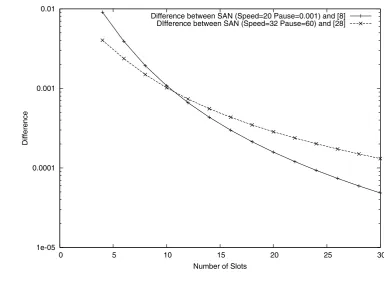
Fig. 4 Difference between continuous space theoretical results and SAN model results
ifx∈ [0,1], andf (x)=0 otherwise, wherep= Pause
Pause+3v1 (2)
Additionally, (2) expresses the probability that a node remains stationary during the whole experiment (pstat), that was not considered for our comparison (we assume pstat=0).
The first validation is a simple comparison with theoret-ical results expressed by (1) usinga=20, i.e., our model with twenty 50 m slots (M=1,000 m andN=20), a very small pause time (Pause=0.001 sec.), and node speed of 20 m/s (rtSpeed=20/50). With this same number of slots, we change the pause time to 60 sec. and the speed to 32 m/s and compared our results with those given by (2). Note that as the size of area used by (2) is 1, the speed (v) used in this equation must be brought in proportion, then we divided the speed in m/s by 1000, which is the size of our area (M).
Numerically speaking, the obtained results have shown the same slot probabilities with a difference around 10e−4. We also tested some small changes in the pause time (from 0.1 to 0.00001 sec.) without having significative changes of probability difference. On the contrary, the choice of the number of slots (N) keeping the same area (M) changes the results considerably. Figure4 shows that assuming from 4 to 30 slots, the difference between probabilities computed by our discrete space model and probabilities found by [7] and [46] theoretical results considering continuous space de-creases exponentially until near 10e−5.
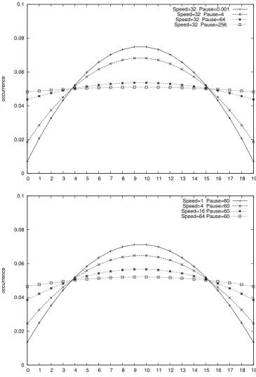
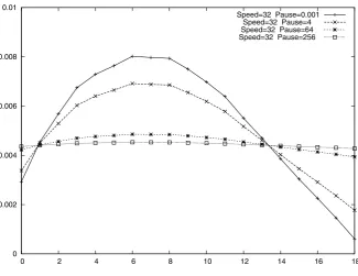
Figure5presents the probability distribution among 20 slots of a 1,000 meters region analyzing the node mobility with a 32 meters per second speed and pause times of 0.001, 4, 64, and 256 seconds. We can observe that as the pause time increases the node spatial distribution spreads more equally in the region, i.e., the result tends to the uniform distribution. This is expected since when the pause time in-creases, the time spent on the path becomes less important than the pause time in the spatial node probability. Since the destination is chosen equiprobably, as the pause time in-creases, the spatial node probability tends to be uniformly distributed.
Another approach analyzed is the node distribution with different speed values. According to [7] and [46], the speed does not affect the distribution considering a zero pause time. Even though we could verify this behavior, we observe that for a more significant pause time (pause=60 sec.) the probability distribution was quite different for dif-ferent speeds (1 m/s, 4 m/s, 16 m/s, and 64 m/s). In fact, Fig. 6 shows a similar effect as observed in vary-ing the pause time, i.e., the more relevant the pause time is in comparison to the node speed, the more close to an equiprobable distribution the result will be. Those re-sults were also consistent with the conclusions presented in [46].
4.2 Random waypoint 2D SAN model
Fig. 5 1D random waypoint spatial node
distribution—varying the pause
Fig. 6 1D random waypoint spatial node
distribution—varying the speed
one node can move to north, south, east, and west. The model representing this 2D movement is presented in Fig.7. This model is obtained through a natural extension from the 1D model of the previous section. The same structure for 1D is replicated, obtaining the four automata that compose the corresponding SAN to the 2D model. In this model, there are two automata to describe the node destination point (DestX andDestY) and two automata to describe the current node location (LocXandLocY). In both pairs of automata, a point
is obtained by ax- andy-coordinate, i.e., the surface is split inN×Nslots.
repre-Fig. 7 Random waypoint 2D SAN model
Fig. 8 Example of routing strategies
sentation (chooseDwas local for the 1D model), the other characteristics of event chooseD are preserved, namely its rate expressed by functionfDand its probability expressed byπ. Note that, functionfD has an analogous way to ex-press if the node is in apausesituation, since it has now to consider the same state in bothxandyaxes, i.e.,
fD=(1/Pause)
∗(stDestX)==(stLocX)
&&(stDestY)==(stLocY)
Another difference between 1D and 2D models is the way to represent the node movement. In the 2D model, the ment is represented by four local events describing move-ments toward north, south, west, and east directions (respec-tively, moveN,moveS,moveW, andmoveE). The rates for those events remain computed as in the 1D model, i.e., ac-cording to the node speed and the slot size. Nevertheless, the expression of this movement event rates needs a more elaborated definition to take routing strategies into account.
The major difference between the 1D and 2D models re-sides in this choice of routing strategy. It is necessary to de-fine whether a node movement may happen in thex- or in they-axis. Note that this need for routing strategy definition is only an important matter due to our model assumption of a node moving in a discrete space. It is clear that the probabil-ity distribution on slots may change according to the chosen routing strategy. For instance, it is intuitive to expect differ-ent probability distribution results to afirstx theny rout-ing, aglutton algorithm routing, or even arandom routing (Fig.8).
The simplest routing strategy to represent in our SAN model is therandomdecision. In that case, we let the choice of axis movement be stochastically decided between two possible events. The model of Fig.7represents this option. Events rates only express if the movement is necessary or not, e.g., eventmoveW is conditioned only by the state of DestXbeing smaller than the state ofLocX.
functional rates of moveN and moveS (y-axis) events to include the restriction to move only if ax movement is no longer needed. The functional rates for eventsmoveN and moveSrespectively should be rewritten as follows:
• fN=rtSpeed∗(((stDestY) < (stLocY))&& ((stDestX)==(stLocX)))
• fS=rtSpeed∗(((stDestY) > (stLocY))&& ((stDestX)==(stLocX)))
The representation of the glutton algorithm strategy is even more elaborated. It allows a node to move only if this movement is in thefarthestdirection to the destination. The four functional rates for events moveW, moveE, moveN, andmoveSshould be rewritten as follows:
• fW=rtSpeed∗(((stDestX) < (stLocX))&& (((stLocX)−(stDestX)) >=
(max((stDestY)−(stLocY), (stLocY)−(stDestY)))))
• fE=rtSpeed∗(((stDestX) > (stLocX))&& (((stDestX)−(stLocX)) >=
(max((stDestY)−(stLocY), (stLocY)−(stDestY)))))
• fN=rtSpeed∗(((stDestY) < (stLocY))&& (((stDestY)−(stLocY)) >=
(max((stDestX)−(stLocX), (stLocX)−(stDestX)))))
• fS=rtSpeed∗(((stDestY) > (stLocY))&& (((stLocY)−(stDestY)) >=
(max((stDestX)−(stLocX), (stLocX)−(stDestX)))))
None of the discrete space routing strategies will pre-cisely describe what happens in a continuous space move-ment. However, the best approximation of the continuous
movement behavior is achieved by the glutton algorithm strategy, specially considering a rather large number of slots.
4.2.1 Validating the 2D model
Analogously to the 1D model, the validation of the 2D can be done by applying it to similar cases presented in [7] and [46]. For that matter, we also analyze a near zero pause time (0.001 sec.) model with 10 meters per sec. speed, a surface of 1000×1000 square meters split in 20×20 slots, and theglutton routingstrategy. Once again the comparison of theoretical results presented in [7,46] with our model’s pre-sented a difference around 10e−4. Also, using the same pa-rameters with a different slot granularity (5×5 and 10×10 slots), we observed the difference decreasing consistently with the 1D comparison (respectively, 10e−2 and 10e−3).
4.2.2 New results for the 2D model—pause vs. speed
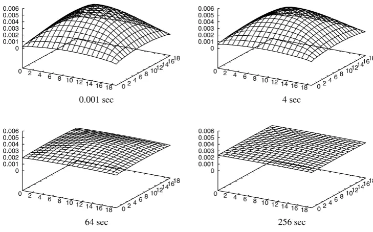
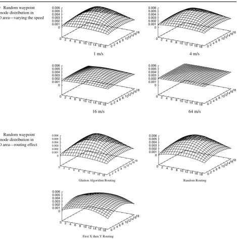
The variations of pause time and speed already made for the 1D case (Figs. 5 and 6) were reproduced with the 1000×1000 surface split in 20×20 slots model also us-ing theglutton algorithm routingstrategy. Figure9 shows the probability distributions obtained for models with a fixed speed (32 m/s) and varying the pause time for 0.001, 4, 64 and 256 seconds. Analogously, Fig.10shows the results for fixing the pause time in 60 sec. and varying the speed for 1, 4, 16, and 64 m/s. Once again, these results show a very similar behavior as the one found for the 1D models, i.e., as the relevance of the pause time increases in comparison with the node speed, the probability distribution tends to be uniform.
Fig. 10 Random waypoint spatial node distribution in 20×20 area—varying the speed
Fig. 11 Random waypoint spatial node distribution in 20×20 area—routing effect
4.2.3 New results for the 2D model—routing strategies
Figure11shows the probability distributions found for the three strategies presented in the previous section (glutton, random,andxtheny) for a model with 1000×1000 square meters surface split in 20×20 slots, node speed of 5 m/s and pause time of 0.001 sec. In opposition to the other ex-periments when a deformation toward equally distributed results were achieved without changing the curves shape, those routing strategies variations do change the distribution shape. It is natural that the greatest effect was found for the x theny strategy, since this choice of routing tends to avoid the central node positions.
4.3 Random waypoint 2D modeling of non-square surfaces
An important feature of SAN is the modular construction that helps the reuse and the replacement of model parts. In this section, we present the results of modeling different convex areas. The proposed SAN model is suitable to de-scribe also areas such as triangles, hexagons (as in [29]), and virtually any polygon. The results obtained to all ir-regular surface models tested have shown consistent be-havior to those previously obtained for square surfaces (Sect.4.2).
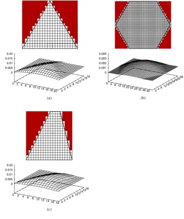
po-Fig. 12 Random Waypoint in a regular and irregular
surface—spatial node
distribution. (a) Triangular area. (b) Hexagonal area.
(c) Trapezium area
sitions, while reachable spots are represent by blank posi-tions. Note that due to the surface discretization, the reach-able slots do not correspond exactly to the expected poly-gon, but merely to an approximation as close as possi-ble.
The unreachable slots modeling is two-fold: functions in event rates prevent or allow nodes to move depending ofx andy-axis in the automataLocXandLocY; and synchroniz-ing events in automataDestXandDestYprevents the choice of a new destination to an unvalid position (an unreachable slot).
The routing strategy used for nonsquare models is a vari-ation of the glutton algorithm, but a slight change was done to prevent node blocking, which may happen in very partic-ular cases near an irregpartic-ular border.
4.3.1 New results for the 2D model—convex polygon surfaces
The modeled areas are presented in the upper part of Fig.12
and their corresponding spatial node distributions are pre-sented in the lower part of the same figure.
To represent a regular triangle we assume 22 slots as base and hypotenuse, and 19 slots as height. The results of the spatial node distribution inside this triangular surface were obtained considering each slot with 50 meters, as in the square area, with node speed of 32 m/s and pause time of 0.001 sec.
Fig. 13 Cross section in middle
y-axis of triangle surface—varying pause
4, 64, and 256 seconds. Figure13shows the probability dis-tributions in the cross section along the middley-axis of the triangle. Similar experiments were performed for a pause time fixed in 60 seconds and speed varying in 1, 4, 16, and 64 m/s, and the results show the same behavior presented in Sect.4.2.1, i.e., as concluded for square models, the propor-tion between pause and speed values seems to be the major drive for the spatial distribution.
Additionally, as validation of our modeling choices, we observe that the curve representing the node distribution for the middley-axis section with speed in 32 m/s and pause time in 0.001 seconds presents a behavior very close to the results presented by Hyytia et al. in [29].
In the hexagonal area, we consider the dimensions of a regular triangle to each sixth part that composes the hexagon. Then the hexagonal area was described inside a rectangular envelope of 44×38 slots. The results presented in Fig.12b were obtained with speed in 32 m/s and pause time in 0.001 seconds.
These same speed and pause values were considered in the results of the trapezium shaped surface (Fig.12c), that lies inside a 19×20 slots envelope. This last example in-tends to stress that unlike the previous results of the litera-ture [29], also irregular surfaces can be modeled as well.
It is also important to observe that the modeling of other surfaces became elegant and natural, needing mainly to spe-cialize the definition of the movement and destination choice transitions, but keeping the main parts of the generic square 2D model. Thus, it is possible to model more realistic sur-faces and to perform predictions about their spatial node dis-tribution. In fact, even non-convex polygons could be mod-eled, but for these cases a more careful definition of the rout-ing strategy functions is needed.
5 Random direction
In this section, we assume the Random Direction mobil-ity model as described by Guerin et al.in [25]. Our analy-sis of the Random Direction mobility model withBounce and Wrap Around, using SAN, resulted in a completely equiprobable spatial node distribution, which is coherent with the literature [5]. Therefore, we concentrate on the Random Direction mobility model with theDelete and Re-placeborder behavior, where non-equiprobable results were found.
Considering that, the behavior of a node is modeled as follows: the node randomly chooses a direction to move with a constant speed, and, after moving during an also randomly chosen duration time, the node makes aPause, then a new choice of direction is done starting this process over and over.
Most of the modeling definitions of the Random Way-point example were kept for both the one- and two-dimens-ional versions of the Random Direction models. Namely, we still divide the surface of interest of size M into N slots, we split the information of node location and its movement in different automata, we model the movement speed and pause duration with ratesrtSpeedandPausefrom the same input parameters information.
5.1 Random direction 1D SAN model
Fig. 14 Random direction 1D SAN model
(i) The node is stopped, represented by stateP in automa-ton Dir. In this case, the node does not move, i.e., automaton Loc does not change its local state, and a choice of direction is the next action. This choice of di-rection is represented by eventchooseD, changing the local state ofDirautomaton to statesW orEwith the same probability.
(ii) The node is moving and it is not yet on a border slot, i.e., either automatonDiris in stateW and automaton Locis in the range 1..N−1, or automatonDiris in state Eand automatonLocis in the range 0..N−2. In this situation, if automatonDiris in stateE, then only the eventmoveEis enabled, representing the movement to East and, of course, the movement toward West is anal-ogous. While moving, the node may stop at any time and go to thepausesituation. Such change of situation is represented by the eventendMovefrom statesEor W to stateP in automatonDir.
(iii) The node is moving and it is on a border slot, i.e., ei-ther automatonDir is in stateW and automaton Loc is in state 0, or automaton Diris in state E and au-tomaton Loc is in state N−1. In this case the node may either stop moving, represented by the possibility of endMove as in the previous situation, or the node may actually cross the border, and then be deleted and replaced by a new node that can be created in any lo-cation. This second possibility is represented by events DelRepEandDelRepW according to the direction the node was moving toward (respectively, East and West). The deleted-and-replaced node continues to move (no pause) and a new choice of direction is made together with the replace, meaning that after a replace the node may move to a different direction. In automatonDir, the choice of the same or a different direction is represented by the two possi-ble (and equiprobapossi-ble) occurrences of eventsDelRepWfrom stateWandDelRepEfrom stateE. That being said, we also
analyze a variant of this behavior in which the node keeps its direction after a delete-and-replace, but the results obtained for both possibilities were exactly equal. In automatonLoc, the occurrence of a delete-and-replace is also represented by either eventDelRepW orDelRepEand it always change from state 0 orN−1 (respectively) to any state.
As said before, the rate for events in the Random Direc-tion model were computed almost always like they were for the Random Waypoint model. This is the case of the chooseDrate that still is the inverse of the pause time, but, unlike the Random Waypoint model, here it does not depend on reach a destination point, i.e.,fD=Pause1 .
Also, the east and west movement rates are calculated according to the numerical value ofrtSpeed tempered by the necessity of the specific direction movement:
fW=(stDir==W )∗rtSpeed
fE=(stDir==E)∗rtSpeed
The event endMoverate is computed as the inverse of the sojourn time of automatonDirin alternatively stateE or stateW, i.e., the expected duration of a movement. This duration could be directly expressed by an input parame-terMoveTime or alternatively by the expected distance of movement (MoveSize) divided by the node speed, i.e.,
fM= 1 MoveTime=
Speed MoveSize
this section): fDR=rtSpeed
5.1.1 Validating the 1D model
To validate the proposed model we consider a 1000 meters region (M=1.000) divided in 20 slots of 50 meters each, and vary the pausetime, the speed, and the size of move-ment.
In the first experiment, we fix the size of movement in 50 meters and vary the speed for 1, 4, 16, and 64 m/s and pause times for 0.001, 16, 64, and 256 seconds. Figure15presents the spatial node distribution for the several combinations of those parameters.
In Fig.15, we also repeat the same combinations of val-ues of speed and pause time with size of movement of 200, 800, and 1600 meters. The first important conclusion ob-tained is that for all combinations of speed and pause time, fixing the size of movement, we observe precisely the same numerical results.
In fact, the variation between the amount of time that a node stays in a slot due to pause and due to movement shows complementary figures, regardless of how much pause time or node speed is assumed. Figure16demonstrates such be-havior by drawing the total node location distribution for all node speeds and pause times combinations (curve T) consid-ering a Size of Movement of 200 meters. The amount spent due to pause and movement for Pause=4 andSpeed=4 (curves P and M) and forPause=4 andSpeed=32 (curves Pand M) are also plotted and one can notice that the results
in curve T are equivalent to the sum of curves P and M, as well as the sum of curves Pand M.
Therefore, we conclude thatPauseandSpeedvalues do not influence the spatial node distribution results for this mo-bility model, using delete-and-replace as border behavior. In fact, the spatial distribution only depends on the size of movement. As the size of movement increases, the spatial node distribution approaches the uniform one.
Using this result we simplify the model presented in Fig.14replacing theDirautomaton (with three states) by a simpler automaton with only two states depicted in Fig.17, where stateP is absent. As said (Sect.3), by reducing the number of automata, or the number of states inside an au-tomaton, the model becomes easier to handle.
This new version of automaton Dir has three events called chooseD, DelRepW, and DelRepE. The events DelRepW andDelRepE have exactly the same function as before, i.e., they are used to model the border behavior.
The event chooseDhas also the same semantics as be-fore. However, in this case, as there is nopause, the new direction choice will be performed as soon as either the size of movement or the moving time finishes. The numerical solution for the model without pause, as expected, is consis-tent with the equivalent continuous space models with pause described in the literature. Numerically speaking, the differ-ence found between our model with or without pause is quite small (around 10e−6 for a 20 slots model).
It is important to notice that the composition of differ-ent automata used in this 1D model, exemplifies one of the greatest advantages of using a structured Markovian formal-ism such as SAN. Namely, the change, replacement, or even
Fig. 16 Pause and movement components in spatial distribution probability
Fig. 17 Dirautomaton for 1D model withoutPause
removal of an automaton usually do not compromise and al-most always do not even affect the definition of the other automata.
5.2 Random direction 2D SAN model
The second proposed SAN model for Random Direction represents a two-dimensional space (Fig.18) and as in the Random Waypoint models, it is a clear extension of the 1D model presented in the previous section. That is the case of the location of the node that was represented by automaton Loc in the 1D model, and now is represented by two au-tomata (LocXandLocY). The surface is divided inN×N slots and the current position of a node is a coordinate given by the local states of automataLocXandLocY.
After building and analyzing several 2D models, with dif-ferent pause times and without pause, we observed that the pause time also does not influence the spatial node distrib-ution in 2D models. This generalizes the results of the 1D model with respect to pause. In consequence, we replace the
automatonDiraccording to Fig. 17. Therefore, in the fol-lowing, we discuss the 2D model without any consideration of pause. Analogously to the 1D case, this modification is modular and does not affect automata corresponding to the node location.
Although several ways can be employed to describe the node direction in a 2D model, the proposed model represents the possible moving directions with one automata (Dir), as well as in the 1D model. However, for the 2D case, Dir represents the possible angles that the node can move. The choice of the angle indicates implicitly the direction chosen (North, South, East, and West). Figure19represents the pos-sible angles considering automatonDirwith sixteen states, i.e., sixteen discrete directions will be considered. Obvi-ously, automatonDircould have any discrete number of di-rections, and such number will define the number of states in automatonDir. Figure18depicts this choice of sixteen states.
Fig. 18 Random direction 2D SAN model
Fig. 19 Axis divided by sixteen directions
endMoveevent in the 1D model and it represents the time a node spends moving. Alternatively, and without any loss of generality, it can represent the distance described by a move step.
The actual move in a 2D area is decomposed in two com-ponents representing the move inX- andY-axis. The rates of eventsMoveE(fE) andMoveW(fW) in automatonLocX and the rates of eventsMoveN(fN) andMoveS(fS) in au-tomaton LocY are adjusted to represent these component speeds, and are represented below:
• fE=SpeedE/SlotSize
• fW=SpeedW/SlotSize
• fN=SpeedN/SlotSize
• fS=SpeedS/SlotSize
These functions depend on the node’s average speed in meters per time unit and the size of the slot in meters (m/N). For instance, the east movement speed is given by the reason between the direction of the node movement (MoveSizeE) and the average time of it (MoveTime):
SpeedE=MoveSizeE MoveTime
The movement direction (MoveSizeE) is decomposed ac-cording to the direction (in degrees). For instance, if a node is moving with speedSp, to the northeast (NE), with 45 de-grees of inclination (counterclockwise), then eventsMoveE andMoveNare both enabled and their rates are respectively calculated according toSp×cosin(α). Considering all pos-sible directions that causes the east movement, the rate as-sociated toMoveSizeEis:
MoveSizeE
=(((stDegree==0)∗(MoveSize))
+(((stDegree==1)||(stDegree==15)) ∗(MoveSize∗0.92387953251))
+(((stDegree==2)||(stDegree==14)) ∗(MoveSize∗0.70710678118))
+(((stDegree==3)||(stDegree==13)) ∗(MoveSize∗0.38268343236)))
Fig. 20 Random direction spatial node distribution in 20×20 area and 16 directions—varying the speed and movement size
the angle approaches 0 degrees. Movement for other direc-tions are similarly implemented.
When a node moves and reaches the border in one of the axis, the Delete and Replace behavior takes place. In both automataLocXandLocY,this behavior is modeled by eventsDelRepN,DelRepS,DelRepE,andDelRepW.
The border behavior defines that a new states inLocXand LocYhave to be equiprobably chosen when one of the events occur. Taking automatonLocXfor explanation, in any of its states it is possible to switch to any of the other states due to DelRepNandDelRepSsince, regardless the horizontal posi-tion the node may be, these vertical reach border events may occur. In state 0, DelRepW can occur and, in stateN −1, DelRepEcan take place depending if the node is moving to west or east respectively. This explains all possible events for each state. The explanation for automatonLocYis anal-ogous.
5.2.1 Validating the 2D model
The results for the 2D model are consistent with those ob-tained for the 1D model and those presented in the liter-ature [5]. They indicate that a more pronounced distribu-tion is in the center area as the movement size or duradistribu-tion are shorter. Analogously, the node distribution tends to be uniform, as the movement duration or size grow. Figure20
presents the spatial node distribution for a model of surface of 1000×1000 meters discretized in 20×20 slots with the same parameters of speed and size of movement presented in [5]. The values of speed considered were 5 and 25 m/s, and movement size considered was 100, 500, 1,000, and 5,000 meters.
However, the comparison with the results in the litera-ture [5] demonstrate that our model gives a little flatter spa-tial node distribution, i.e., our predictions seems to have a less pronounced probability to find a node in the central area. We believe that this happen due to the number of directions considered (sixteen).
5.2.2 New results for the 2D model—varying the number of directions
It is important to remind that our model assumes a discrete number of directions. Figure 21 depicts the variations in the node distribution when smaller or greater (4, 8, 12, and 20) number of directions are considered. The first plot of Fig.20complements Fig.21with information for 16 direc-tions.
A closer look in these results is presented in Figs. 22
and23. They present middle sections on the surfaces cor-responding to the results with 4, 8, 12, 16, and 20 directions, where Fig.22shows these sections in the 5 central slots and Fig.23 shows these sections for slots in the periphery of the 20 × 20 area. As can be observed, as the number of directions increases the impact on the results becomes less significant.
6 Conclusion
Fig. 21 Random direction spatial node distribution in 20×20 area with Speed=5 and Movement
Size=100—varying the number of directions
Fig. 22 Middle sections on the surfaces corresponding to the results with 4, 8, 12, 16, and 20 directions—5 central slots
by showing their numerical compatibility with existing an-alytical or simulation studies to the closest cases, i.e., the cases where a continuous surface was considered. Besides showing the suitability of SAN to the modeling of these mobility models, we have contributed to the better under-standing of detailed aspects in the Random Waypoint such as pause time, node speed, and routing strategies in the 2D node distribution, especially considering a discrete mobility space.
We would like to stress the fact that all results presented in this paper were obtained by numerical solution of the SAN models, and not by any simulation technique. This fact enhances the contribution of this paper since the SAN
mod-eling delivers more reliable results from a statistical point of view.
In the Random Direction, we have contributed to show that spatial node distribution is influenced by movement du-ration and that the speed and pause time do not influence the distribution. We also noticed that the (discrete) number of directions a node can move is relevant to the spatial distrib-ution.
Fig. 23 Middle sections on the surfaces corresponding to the results with 4, 8, 12, 16, and 20 directions—peripheryc slots
Fig. 24 Random waypoint spatial node distribution in 3D
It is important to observe that we could modularly ex-tend the SAN models to consider much more detailed ad-ditional aspects such as varying speed according to accel-eration, slower/faster areas, or different pause time per po-sition could be easily modeled. Actually, any other nonuni-form behavior could be considered. Moreover, since we use automata networks, we can step-wise include more dimen-sions adding more automata and also adding some complex-ity to functions. Experimental three-dimensional space with Random Waypoint mobility model was described including two more automata to the 2D model. This last experiment considers a 8×8×8 slots describing a space of 1 km3, near
zero pause time (0.001 sec.) and 10 meters per sec. speed. Figure24represents the spatial node distribution for the dis-crete slices inzaxis. As expected, we found a higher proba-bility of the node to be in the central slots of the solid region, i.e., in the center of the slices surfaces and in the central slices (z=3 and 4).
for-malism. In the future, we intend to model more complex realities, such as buildings with obstacles. In fact, obstacles can be suitably modeled in SAN through functional rates as-signed to the transitions and reachability functions that limit reachable spots.
Natural future works, besides the ones already men-tioned, are the use of the spatial node distributions achieved to obtain performance and dependability levels of such net-works. Moreover, some numerical studies could be carried out to achieve more efficient spatial distribution predic-tions. For example, we could study stochastic properties of nearly independent automata (automata without synchroniz-ing events) in order to derive product-form solutions, or at least solutions numerically more efficient. Such improved solutions could significantly reduce the computational cost to solve large complex models like the hexagon (Fig.12c). This model, the largest solved within this paper, represents a 2.8 million states model, and it takes about a day to be solved in a small workstation, i.e., Xeon 2.2 GHz with 512 Mbytes cache and 2 Gbytes of RAM memory. Smaller models, like the Random Waypoint with 20×20 slots (a model with 160 thousand states) are usually solved in less than 30 minutes in the same machine. Recent improvements in dealing with structured models [16] could significantly reduce this so-lution times, but even with current software [10] the SAN models already offer valid insights with an affordable com-putational cost for quite large examples.
Acknowledgements The authors wish to express their gratitude to Fábio Delamare for early discussions in the topics of this paper.
References
1. Abolhasan M, Wysocki T, Dutkiewicz E (2004) A review of rout-ing protocols for mobile ad hoc networks. Ad Hoc Netw 2(1):1– 22
2. Ajmone Marsan M, Conte G, Balbo G (1984) A class of general-ized stochastic petri nets for the performance evaluation of multi-processor systems. ACM Trans Comput Syst 2(2):93–122 3. Bansal N, Liu Z (2003) Capacity, delay and mobility in wireless
ad-hoc networks. In: IEEE Infocom
4. Benchaïba M, Bouabdallah A, Badache N, Ahmed-Nacer M (2004) Distributed mutual exclusion algorithms in mobile ad hoc networks: an overview. Oper Syst Rev 38(1):74–89
5. Bettstetter C (2001) Mobility modeling in wireless networks: Cat-egorization, smooth movement, and border effects. Mob Comput Commun Rev 5(3):55–66
6. Bettstetter C (2001) Smooth is better than sharp: a random mo-bility model for simulation of wireless networks. In: Proceedings of the 4th ACM international workshop on Modeling, analysis and simulation of wireless and mobile systems. ACM, New York, pp 19–27
7. Bettstetter C, Resta G, Santi P (2003) The node distribution of the random waypoint mobility model for wireless ad hoc networks. IEEE Trans Mob Comput 2(3):257–269
8. Bettstetter C, Hartenstein H, Perez-Cost X (2004) Stochastic properties of the random waypoint mobility model. Wirel Netw 10(5):555–567
9. Brenner L, Fernandes P, Sales A (2005) The need for and the ad-vantages of generalized tensor algebra for Kronecker structured representations. Int J Simul Syst Sci Technol 6(3–4):52–60 10. Brenner L, Fernandes P, Plateau B, Sbeity I (2007) PEPS 2007—
Stochastic Automata Networks Software Tool. In: International conference on quantitative evaluation of systems (QEST 2007). IEEE Press, New York, pp 163–164
11. Broch J, Maltz DA, Johnson DB, Hu Y, Jetcheva J (1998) A per-formance comparison of multi-hop wireless ad hoc network rout-ing protocols. In: Proceedrout-ings of the fourth annual ACM/IEEE int conf on mobile computing and networking (MobiCom). ACM Press, New York, pp 85–97
12. Buchholz P, Ciardo G, Donatelli S, Kemper P (2000) Complexity of memory-efficient Kronecker operations with applications to the solution of Markov models. INFORMS J Comput 12(3):203–222 13. Camp T, Boleng J, Davies V (2002) A survey of mobility
mod-els for ad hoc network research. Wirel Commun Mob Comput 2(5):483–502. Special issue on Mobile Ad Hoc Networking: Re-search, Trends and Applications
14. Choffnes DR, Bustamante FE (2005) An integrated mobility and traffic model for vehicular wireless networks. In: Proceedings of the 2nd ACM int. workshop on vehicular ad hoc networks, VANET ’05. ACM, New York, pp 69–78
15. Chu T, Nikolaidis I (2004) Node density and connectivity prop-erties of the random waypoint model. Comput Commun 27:914– 922
16. Czekster RM, Fernandes P, Webber T (2009) GTAEXPRESS: a software package to handle Kronecker descriptors. In: QEST’09: quantitative evaluation of systems
17. Czekster RM, Fernandes P, Sales A, Taschetto D, Webber T (2010) Simulation of Markovian models using Bootstrap method. In: Pro-ceedings of the 2010 summer computer simulation conference (SCSC ’10). pp 564–569
18. Czekster RM, Fernandes P, Sales A, Webber T (2011) A mem-ory aware heuristic for fast computation of structured Markovian models through tensor product restructuring. Numer Linear Alge-bra Appl (to appear)
19. Czekster RM, Fernandes P, Webber T (2011) Efficient vector-descriptor product exploiting time-memory trade-offs. ACM SIG-METRICS Perform Eval Rev (to appear)
20. Delamare F, Dotti FL, Fernandes P, Nunes CM, Ost LC (2006) An-alytical modeling of random waypoint mobility patterns. In: PE-WASUN ’06: proceedings of the 3rd ACM international workshop on performance evaluation of wireless ad hoc, sensor and ubiqui-tous networks. ACM, New York, pp 106–113
21. Di W, Xiaofeng Z, Xin W (2006) Analysis of 3-d random direction mobility model for ad hoc network. In: ITS telecommunications proceedings, 6th int conf on, pp 741–744
22. Doyle SJ, Forde TK, Doyle LE (2006) Spatial stationarity of link statistics in mobile ad hoc network modelling. In: MASCOTS ’06: proceedings of the 14th IEEE international symposium on mod-eling, analysis, and simulation. IEEE Comput Soc, Washington, pp 43–50
23. Fuggetta A, Picco GP, Vigna G (1998) Understanding code mobil-ity. IEEE Trans Softw Eng 24:342–361
24. González MC, Hidalgo CA, Barabási A-L (2008) Understanding individual human mobility patterns. Nature 453(7196):779–782 25. Guérin RA (1987) Channel occupancy time distribution in a
cel-lular radio system. IEEE Trans Veh Technol 36:89–99
26. Haas ZJ, Pearlman MR (1998) The performance of query con-trol schemes for the zone routing protocol. In: ACM SIGCOMM. pp 167–177
27. Hillston J (1996) A compositional approach to performance mod-elling. Cambridge University Press, New York
29. Hyytia E, Lassila P, Virtamo J (2006) Spatial node distribution of the random waypoint mobility model with applications. IEEE Trans Mob Comput 5(6):680–694
30. Jardosh A, Belding-Royer E, Almeroth K, Suri S (2003) Towards realistic mobility models for mobile ad hoc networks. In: Proceed-ings of the 9th annual international conference on mobile comput-ing and networkcomput-ing. ACM, New York, pp 217–229
31. Jardosh A, BeldingRoyer EM, Almeroth KC, Suri S (2003) To-wards realistic mobility models for mobile ad hoc networks. In: MobiCom ’03: proceedings of the 9th annual int conf on mobile computing and networking. ACM, New York, pp 217–229 32. Jayakumar G, Ganapathi G (2008) Reference point group mobility
and random waypoint models in performance evaluation of manet routing protocols. J Comput Syst Netw Commun
33. Kemper P (1996) Numerical analysis of superposed GSPNs. IEEE Trans Softw Eng 22(9):615–628
34. Kleinrock L, Silvester J (1978) Optimum transmission radio for packet radio networks or why six is a magic number. In: Proc of the IEEE national telecommunications conf
35. Kumar M, Rajesh RS (2009) Performance analysis of manet rout-ing protocols in different mobility models. Int J Comput Sci Netw Secur 9(2):22–29
36. Lassila P, Hyytiä E, Koskinen H (2005) Connectivity properties of random waypoint mobility model for ad hoc networks. In: Pro-ceedings of the fourth annual Mediterranean workshop on ad hoc networks (Med-Hoc-Net)
37. Le Boudec J, Vojnovic M (2005) Perfect simulation and stationar-ity of a class of mobilstationar-ity models. In: INFOCOM 2005. 24th annual joint conf of the IEEE computer and communications societies. Proceedings IEEE, vol 4. IEEE Press, New York, pp 2743–2754 38. Lin G, Oubir G, Rajaraman R (2004) Mobility models for ad hoc
network simulation. In: IEEE infocom
39. Malpani N, Welch JL, Vaidya N (2000) Leader election algorithms for mobile ad hoc networks. In: DIALM ’00: proceedings of the 4th international workshop on discrete algorithms and methods for mobile computing and communications. ACM, New York, pp 96– 103
40. Milner R (1999) Communicating and mobile systems: the π -calculus. Cambridge University Press, Cambridge
41. Nain P, Towsley D, Liu B, Liu Z (2005) Properties of random di-rection models. In: IEEE Infocom, pages. IEEE Press, New York, pp 1897–1907
42. Navidi W, Camp T (2004) Stationary distributions for the random waypoint mobility model. IEEE Trans Mob Comput 3(1):99–108 43. Nilsson A (2004) Performance analysis of traffic load and node
density in ad hoc networks. In: Proceedings of the 5th European wireless 2004: mobile and wireless systems beyond 3G
44. Plateau B (1985) On the stochastic structure of parallelism and synchronization models for distributed algorithms. ACM SIG-METRICS Perform Eval Rev 13(2):147–154
45. Rajaraman R (2002) Topology control and routing in ad hoc net-works: a survey. SIGACT News 33(2):60–73
46. Resta G, Santi P (2002) An analysis of the node spatial distribution of the random waypoint mobility model for ad hoc networks. In: POMC ’02: proceedings of the second ACM international work-shop on principles of mobile computing. ACM, New York, pp 44– 50
47. Royer EM, Melliar-Smith PM, Moser LE (2001) An analysis of the optimum node density for ad hoc mobile networks. In: IEEE international conference on communications, vol 3. pp 857–861 48. Saha AK, Johnson DB (2004) Modeling mobility for vehicular
ad-hoc networks. In: Proceedings of the 1st ACM int. workshop on vehicular ad hoc networks, VANET ’04. ACM, New York, pp 91– 92
49. Santi P, Blough DM (2002) An evaluation of connectivity in mo-bile wireless ad hoc networks. In: DSN ’02: proceedings of the 2002 international conference on dependable systems and net-works. IEEE Comput Soc, Washington, pp 89–102
50. Stewart WJ (2009) Probability, Markov chains, queues, and simu-lation. Princeton University Press, Princeton