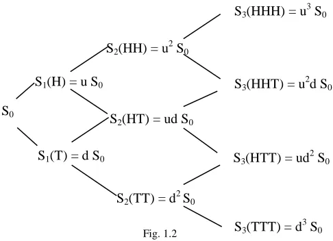
S0
S1(H) = u S0
S1(T) = d S0
S2(HH) = u 2
S0
S2(HT) = ud S0
S2(TT) = d2 S0
S3(HHH) = u3 S0
S3(HHT) = u2d S0
S3(HTT) = ud2 S0
S3(TTT) = d3 S0
Fig. 1.2
Some Computational Aspects of Martingale
Processes in ruling the Arbitrage from
Binomial asset Pricing Model
Sheik Ahmed Ullah
Abstract— This paper concerns about some computational aspect of martingale processes in binomial asset pricing models. Mathematica programs are incorporated to get the martingale values, which lead to no-arbitrage option values through first fundamental theorem of asset pricing, for a set of risk neutral probabilities. Numerical example, through Mathematica program, ensures the theoretical fact that if not discounted properly the underlying stock price dynamics doesn’t follow martingale process.
Index Terms—risk neutral probability, martingale, arbitrage, option price, discounting.
I. INTRODUCTION
Arbitrage plays an important role in the dynamics of a stock market. Before investing money in any particular stock market it is very important to check about its existence. For a proper economy we should always try to rule out any kind of arbitrage. Asset pricing models having underlying processes as martingale, rules out the existence of arbitrage, hence the study of martingale becomes vital. In this paper probability measure and conditional expectation are introduced to carry their intuitions in martingale process. Extensive programming efforts are incorporated through different Mathematica
programs.
II.LITERATURE SURVEY
Binomial model for Stock prices:
For one period fixed fluctuation Binomial model, we consider t = 0 at starting and t = 1 for the end of period, S0 as the stock
price per share at t = 0 with S0 > 0, S1 as the stock price per
share at t = 1, u as up factor of a stock price for one period, d as down factor of a stock price for one period, p as the probability of the increase of a stock price at next period, q as the probability of the decrease of a stock price at next period. Which leaves us with p = 1 – q.
Sheik Ahmed Ullah is with the Department of Mathematics and Natural Sciences, BRAC University, BANGLADESH as Lecturer.
(email: [email protected] or [email protected])
Since the event of Stock price’s increasing or decreasing is random, we are considering that a coin is tossed and the outcomes of the coin determine the price. Hence we get the following mathematical frame work for a Multi-period Binomial Model (in this case for three periods) where Head(H) as an output of the coin toss event means the increase of the stock price by the up factor u and Tell(T) means the decrease of the stock price by the down factor d.
Suppose, we begin with wealth X0 and buy Δ0 shares of stock
at time zero. If Δ0S0 ≥ X0 then we have to borrow (Δ0S0-X0)
from the money market at interest rate r. Then the value of our portfolio of stock and money market at time one will be,
p
q
S1 = uS0
S1 = dS0
S0
t = 0 t = 1
X1 = Δ0 S1 + (1 + r) (X0 - Δ0S0) = (1+r) X0 + Δ0 [S1-(1+r) S0]
Here we can divide X1 in to risky part Δ0S1 and risk free part
(1 + r) (X0 - Δ0S0). Particularly,
X1(H)= Δ0 S1 (H) + (1 + r) (X0 - Δ0S0)
X1(T)= Δ0 S1 (T) + (1 + r) (X0 - Δ0S0)
Here we are not using any argument for X0 and S0 since X0
and S0 are not actually random. The randomness occurs only
for X1 and S1. So without randomness the term, (1 + r) (X0 -
Δ0S0) become risk less and the term Δ0S1 is the risky part since
S1 can be either S1(H) or S1(T). So clearly X1 is another
random variable.
We want to choose X0 and Δ0 in a way so that X1(H) = V1(H)
and X1(T) = V1(T) where V1(H) = u S0 and V1(T) = d S0 are
known as we have given the payoff function of the derivatives security for this one period model. Thus replicating the derivative security requires that
X0+ Δ0 (
r
1
1
S1 (H) – S0) =
r
1
1
V1(H) (1.1)
X0+ Δ0 (
r
1
1
S1 (T) – S0) =
r
1
1
V1(T) (1.2)
Now we will solve the equation for X0 and Δ0.
Multiplying (1.1) by
p
~
and (1.2) byq
~
= 1 –p
~
and adding them we getX0 + Δ0 (
r
1
1
[
p
~
S1(H)+q
~
S1(T)] – S0)=
r
1
1
[
p
~
V1(H) +q
~
V1(T)] (1.3)If we choose
p
~
in a way thatS0 =
r
1
1
[
~
p
S1 (H) +q
~
S1(T)] (1.4)then the term multiplying Δ0 in (1.3) is zero and we have a
simple formula for X0
X0 =
r
1
1
[
p
~
V1(H) +q
~
V1(T)]We can solve
p
~
directly from (1.4) in the form
u
d
p
d
r
S
dS
p
uS
p
r
S
~
)
(
1
)
~
1
(
~
1
1
0
0 0
0
This leads to the formulas:
p
~
=d
u
d
r
1
and
q
~
=d
u
r
u
1
We call
~
p
andq
~
as the Risk neutral probabilities.Under the actual probabilities, the average rate of growth of the stock is typically strictly greater than the rate of growth of the same amount’s investment in the money market. Otherwise no one would want to incur the risk associated with investing in money market. So for the actual probability p and q = 1 – p.
p S1(H) + q S1(T) > (1+r) S0
in Stock market in Money market
S0 <
r
1
1
[
p
S1(H) +q
S1(T)]Whereas we chose
~
p
andq
~
= 1 -p
~
in such a way so that it satisfiesS0 =
r
1
1
[
~
p
S1(H) +q
~
S1(T)]
(1+r)S0 =~
p
S1(H) +
q
~
S1(T)
money market investment. Then the investors must be neutral about risk (they do not require compensation for assuming it nor they are willing to pay extra for it.). Hence the name risk neutral probabilities.
p
~
=d
u
d
r
1
and
q
~
=d
u
r
u
1
(1.5)
We call the number
p
~
andq
~
as risk neutral probabilities and the equation.V0 =
r
1
1
[
p
~
V1(H) +q
~
V1(T)] (1.6)as risk neutral pricing formula where the actual probabilities are absent.
For such use of risk neutral probabilities in risk neutral pricing formula the prices of the derivative security in the Binomial model depends only on the set of possible stock price paths, (pricing formula V0 uses all V1 ( ) where ( ) represents all
possible stock price paths) but not on how probable these paths are. i.e. the probability of none of these paths appearing in the pricing formula.
Arbitrage free market:
Arbitrage is a trading strategy that begins with no money, has zero probability of losing money and has a positive probability of making money. By this trading strategy wealth can be generated from nothing. A market which is free from arbitrage is called arbitrage free market.
A mathematical model that admits arbitrage negatively influences the mathematical analysis. From mathematical point of view, an arbitrage free market must hold the following inequalities,
0 < d < (1+ r) < u
Where, r is the interest rate in the money market. Here we recall the one period fixed fluctuation model to explain these inequalities.
Note: d > 0 as the stock prices are always positive.
Explanation of d < (1 + r):
At first we assume the situation when d ≥ (1 + r). Now if one begin with zero wealth and at time t = 0 borrows S0 from the
money market in order to buy stock, then he has to pay the money market (1 + r) S0 at time t = 1, while in the worst stock
price fall he will get dS0 which is greater than or equal to (1 +
r) S0, since d ≥ (1 + r) => dS0 ≥ (1 + r) S0.
And if the stock price increases he will get uS0 which is
strictly greater than (1+r) S0, since u > d ≥ (1+r) ≥ uS0 > (1+r)
S0, So for all sorts of fluctuation of stock prices he has the
ability to pay off the money market debt and has a positive probability to gain wealth from nothing.
This provides an arbitrage. So we must have d < (1+r) for arbitrage free market.
Explanation of u > (1+ r):
Similarly we consider the situation for u ≤ (1+r). Now if one sells the stock at time zero and invest the money in the money market, at the time one he will get (1+r) S0 from the money
market while in the best case, the cost of replacing the stock is uS0 which is less than value of the money market return. Thus
he has the stock at time t = 1, as he had at the time t = 0 plus he may have some profit from the money market, so this also provides an arbitrage. So we must have u > (1+r) for arbitrage free market.
Expected values (mathematical expectations):
If X is a random variable defined over the sample space, Ω = {ω1,ω2…………. ωn} with corresponding probabilities
P(ω1),P(ω2)………..P(ωn) then the expected value, i.e. the
mathematical expectation of X, is symbolically defined as
n
i
i i
1
) P( ) ( X ) )P( ( X X) ( E
Discounted process and Expected value:
Recalling from the multi period Binomial model and the equation (1.6) at every time n and for every sequence of coin tosses ω1, ω2……. ωn , we have
Sn (ω1,ω2……... ωn) =
r
1
1
p Sn+1 (ω1, ω2, ….. ωn, ) + q Sn+1 (ω1, ω2……. ωn,,T )]
The stock price at time n is the discounted weighted average of the two possible stock prices at time t = n + 1, where thep q
are the weights used in the averaging. So the expected value of Sn+1 at time t = n is,
p Sn+1 (ω1, ω2, … ωn ) + q Sn+1 (ω1, ω2…. ωnT )
From (2.1) & (2.2 )we have Sn =
r
1
1
n [Sn+1]
Conditional Expectation:
The conditional expectation of a stock price Sm at time t = n,
where (n < m) is the expected values of all possible values of Sm at time t = n, conditioned by their information we need at
time t = n. We denote it by
E
n[
S
m]
.In general let n satisfy 1 ≤ n ≤ N and let ω1, ω2,……….,ωn be
given and for the moment fixed. There are 2N-n possible continuations ωn+1, ωn+2………..,ωN of the fixed sequence
ω1, ω2,………….,ωn. denoted by # (ωn+1, ωn+2………..,ωN )
the number of heads in the continuation ωn+1,
ωn+2………..,ωN and denoted by # T(ωn+1, ωn+2………..,ωN
) the number of tails.
En X]( ω1, ω2,……….,ωN) =
N
n
N n N n
N n n
X
q
p
. ,...
1 1
) ,... ( # ) ,.. ( #
1
1
1
(
,....
...
)
(1.7)
Based on what we know at time zero, the conditional expectation En [X] is random in the sense that its value
depends on the first n coin tosses, which we do not know until time n.
The two extreme cases of conditioning are E0[X], the
conditional expectation of X based on no information, which we define by, E0[X] = EX, where EX means the total
expectation using complete continuations ω1, ω2, …, ωn , ωn+1,
ωn+2………..,ωN and EN[X] the conditional expectation of X
based on knowledge of all n coin tosses, which are defined by En [X] = X, which is obtained by no continuations.
Martingale:
In probability theory, a martingale is a stochastic process (i.e. a sequence of random variables) such that the conditional expected value of an observation at some time t, given all the observations up to some earlier time s, is equal to the observation at that earlier time s.
Consider the Binomial asset pricing model. Let M0, M1, M2, ………. MN be a sequence of random variables, with each MN
depending on random evolution up to times n (i.e.M0
constant). Such a sequence of random variables is called a Martingale stochastic process,
if Mn = En [Mn+1] , n = 0 ,1, 2………N-1
i.e. for martingale process the conditional expected value of the next observation, given all the past observations, is equal to the last observation.
Sub-martingale:
The above process (M0, M1, M2, ………. MN)is called as sub
martingale if Mn
En [Mn+1], for n = 0,1, 2…...N-1Super-martingale:
The above process (M0, M1, M2, ……. MN)is called as super
martingale if Mn
En [Mn+1], for n = 0 ,1, 2…...N-1First fundamental theorem of Asset pricing:
“If we can find a risk- neutral measure in a model (i.e. a measure that agrees with the actual probability measure about which paths have zero probability and under which the discounted prices of all primary assets are martingale), then there is no arbitrage in the model.”
The main importance of this theorem is in ruling out the arbitrage from the market.
III. OBJECTIVE OF THE STUDY
The main objective of this study is to design a structure based on the first fundamental theorem of Asset pricing to identify the existence of any arbitrage in a stock market. Here we are trying find a nice graphical representation using necessary known inputs like initial stock price, up factor and down factor (which can be predicted from the underlying asset’s history), So that the existence of arbitrage is easily detectable.
IV. METHODOLOGY
A program in Mathematica generated by using the last formula stated may be used to determine conditional expectation for any time period. The conditional expectation of S6 based on
the information available at time t = 3, was determined by the program as,
2621
.
79
)
55
.
66
](
[
)
](
[
6 3 63
S
HHH
E
S
E
8948
.
69
)
685
.
58
](
[
)
](
[
6 3 63
S
HHT
E
S
E
6345
.
61
)
7495
.
51
](
[
)
](
[
6 3 63
S
THT
E
S
3504
.
54
)
6337
.
45
](
[
)
](
[
6 3 63
S
TTT
E
S
E
where the inputs were, initial stock price S0 = 50, up factor u =
1.1, down factor d = 0.97, interest rate r = 0.06.
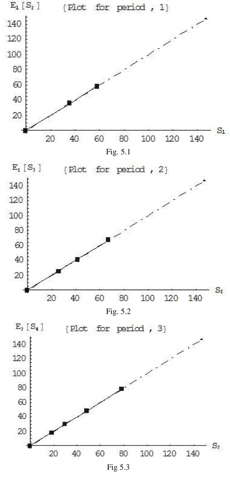
If we plot Mn along horizontal axes (X axes) and En[Mn+1]
along vertical axes (Y axes) i.e. if (Mn , En[Mn+1] ) represents a
point in that rectangular plane, then when the process Mn is
martingale X co-ordinate and Y co-ordinate of every points are equal and so every point will lie on the diagonal line. If the process is super martingale then the points will lie above the diagonal line and for sub martingale they will lie below the diagonal.
V. ANALYSIS AND FINDINGS
First let us verify for discounted stock price and risk neutral probability. When the program runs the input box will appear with the tags as follows.
“Input the number of last period”
We enter 8. (but this program will work for any number of periods)
Then it asks for the types of the input. In this case if we want to use the input as 1 then the program will ask for the specific values of stock price, up & down factor, interest. Otherwise we use the input is 0 (zero) to use the default values as follows,
Stock price S0 = 50
Up factor u = 1.3 Down factor d = 0.8
Interest rate (money market) r = 0.12.
The next option is to decide about to check for the Stock price (input 1) or Discounted stock price (input 2). We choose the 2nd option.
The last option is to decide about choice of kind of probability. We can use either risk neutral probability (input 1) or random probability (input 2).
Here the program generates probability randomly using the command “Random ]” of Mathematica that returns random number between 0 ( zero ) and 1. Finally we get the following output.
921
.
141
)
921
.
141
](
[
)
](
[
8 7 87
S
HHHHHHH
E
S
E
3361
.
87
)
3361
.
87
](
[
)
](
[
8 7 87
S
HHHHHHT
E
S
E
7453
.
53
)
7453
.
53
](
[
)
](
[
8 7 87
S
THHHHHT
E
S
E
074
.
33
)
074
.
33
](
[
)
](
[
8 7 87
S
TTHHHHT
E
S
E
3533
.
20
)
3533
.
20
](
[
)
](
[
8 7 87
S
TTTHHHT
E
S
E
5251
.
12
)
5251
.
12
](
[
)
](
[
8 7 87
S
TTTTHHT
E
S
E
70774
.
7
)
70774
.
7
](
[
)
](
[
8 7 87
S
TTTTTHT
E
S
E
74323
.
4
)
74323
.
4
](
[
)
](
[
8 7 87
S
TTTTTTT
E
S
E
---
Fig. 5.1
Fig. 5.2
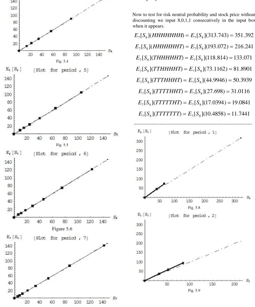
Fig. 5.4
Fig. 5.5
Figure 5.6
Fig. 5.7
Since every point is lying on the diagonal line the process is a Martingale process.
Now to test for risk neutral probability and stock price without discounting we input 8,0,1,1 consecutively in the input box when it appears.
392
.
351
)
743
.
313
](
[
)
](
[
8 7 87
S
HHHHHHH
E
S
E
241
.
216
)
072
.
193
](
[
)
](
[
8 7 87
S
HHHHHHT
E
S
E
071
.
133
)
814
.
118
](
[
)
](
[
8 7 87
S
THHHHHT
E
S
E
8901
.
81
)
1162
.
73
](
[
)
](
[
8 7 87
S
TTHHHHT
E
S
E
3939
.
50
)
9946
.
44
](
[
)
](
[
8 7 87
S
TTTHHHT
E
S
E
0116
.
31
)
698
.
27
](
[
)
](
[
8 7 87
S
TTTTHHT
E
S
E
0841
.
19
)
0394
.
17
](
[
)
](
[
8 7 87
S
TTTTTHT
E
S
E
7441
.
11
)
4858
.
10
](
[
)
](
[
8 7 87
S
TTTTTTT
E
S
E
---
Fig. 5.8
Fig. 5.10
Fig. 5.11
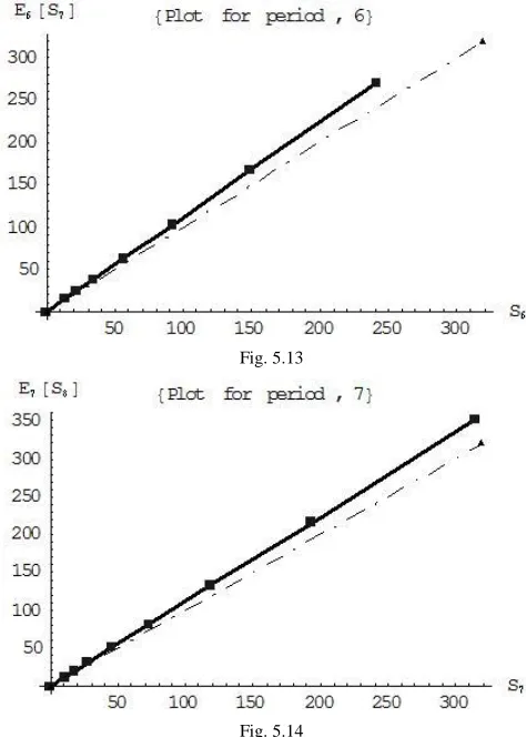
Fig. 5.12
Fig. 5.13
Fig. 5.14
Since every point is lying over the diagonal line the process is a super-martingale process.
For stock price process under random probability we input consequently 8,0,1,2 where the random probability p > p` where p` is the solution of the equations[1],
p` × u + q` × d = 1, p` + q` = 1 (5.1) to get the following output
508
.
273
)
743
.
313
](
[
)
](
[
8 7 87
S
HHHHHHH
E
S
E
313
.
168
)
072
.
193
](
[
)
](
[
8 7 87
S
HHHHHHT
E
S
E
577
.
103
)
814
.
118
](
[
)
](
[
8 7 87
S
THHHHHT
E
S
E
7396
.
63
)
1162
.
73
](
[
)
](
[
8 7 87
S
TTHHHHT
E
S
E
2244
.
39
)
9946
.
44
](
[
)
](
[
8 7 87
S
TTTHHHT
E
S
E
1381
.
24
)
698
.
27
](
[
)
](
[
8 7 87
S
TTTTHHT
E
S
E
8542
.
14
)
0394
.
17
](
[
)
](
[
8 7 87
S
TTTTTHT
E
S
E
14105
.
9
)
4858
.
10
](
[
)
](
[
8 7 87
S
TTTTTTT
E
S
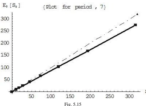
Fig. 5.15
Which is the graph for the last period only. Since every point is lying under the diagonal line this process is a sub-martingale process.
VI. DISCUSSIONS
It has been observed that if we run the program frequently for the series of inputs as 8,0,1,2 using random probability instead of risk neutral probability, sometimes it shows stock price process is super martingale and sometimes sub martingale. So there exists a probability measure for which stock price process is martingale. From the theoretical point of view[1] the measure is obtained by solving the equations 5.1.
It is observed that when the value of p assigned by the random number generator “Random ]” = p > p` the stock price process is super martingale and when p < p` the stock price process is sub martingale. Here for the default values of the parameters u = 1.3 and d = 0.8, the value of p` is 0.4 which is obtained by solving the equations 5.1 and p = 0.143517 assigned by the random number generator. As a result in the last graph it shows that the stock price process is sub martingale.
So “p(random)<p`” leads the stock price process to sub martingale and “p(random)>p`” leads the stock price process to super martingale. And for a variable to be martingale the Sn+1 VS En[Sn+1] graph must coincide with the diagonal line
for every value of n.
But if we consider the stock price which is super martingale for the given set of data, it is observed that with the increase of n (number of period) the slope of the straight line increases i.e. the ratio of expectation of the stock price at next period (n+1) with the stock price at n is increasing with the increase of stock price. So the quantity of gained money by an arbitrager will increase with the increase of stock price i.e. He or she will gain as more as the stock price when the stock price is super martingale. The same reason will explain the loss of an arbitrager in case of sub martingale.
VII. CONCLUSION
Confinement to the discrete settings is motivated by the fact that grasping the intuitions is convenient in discrete settings. The intuitions like risk-neutral probabilities, conditional expectations, martingale and different stochastic processes (involved in discrete time binomial asset pricing model) as explored and programmed paves the path of assuming further research in many of the challenging directions of Mathematical Finance. The intuition of measurability is also important for the functions of random variable and for the stochastic process in this context. Other asset pricing models like Black-Scholes model, Cox-Ingersoll-Ross model (CIR model) etc. which are still in use in the market with some changes can be used to explore similar ideas through the method used in this paper.
REFERENCES
[1] Shreve,Steven, 2004. Stochastic Calculus for Finance- I: The Binomial Asset Pricing Model. Springer Finance.R.
[2] Hull, C, John, 2006. Options, Futures and Other Derivatives, 6/E. [3] Benninga Simon and Wiener Zvi. 1997. The Binomial Option Pricing
Model, Mathematics in Education and Research(MiER), Vol. 6, No. 3 [4] Benninga Simon and Wiener Zvi. 1997. Binomial Option Pricing, the
Black-Scholes option Pricing Formula and Exotic Option. Mathematics in Education and Research (MiER), Vol. 6, No. 4, pp. 11-14.
[5] Roussas, G. George, 2005, An Introduction to Measure-theoretic Probability. Elsevier Academic press.
[6] Cox J.C., Ross S. A., Rubinstein M., 1979, Option Pricing: A simplified approach, Journal of Financial Economics, Vol. 7, pp. 229-263. [7] Dietmar P. J. and Matthias Reimer, 1996, Binomial models for option
valuation- examining and improving convergence, Applied Mathematical Finance, Vol. 3, Issue 4, pp. 319-346.
[8] Rangarajan K. Sundaram, 1997, Equivalent Martingale measure and risk-neutral pricing an expository note, The Journal of Derivatives, Vol. 5, No. 1, pp. 85-98.
[9] Stanly R. Pliska, 2001, Introduction to Mathematical Finance Discrete time models, Black well publishing.