Low Memory Set-Partitioning in Hierarchical Trees Image Compression Algorithm

Abstract— The Set Partitioning in Hierarchical Trees (SPIHT) image compression algorithm is very efficient, has low

computational complexity, and generates an embedded

compressed bit-stream that can be efficiently decoded at several data rates (qualities). Unfortunately it needs a huge amount of computer memory due to using three linked lists to store the coordinates of the image pixels. In addition the S PIHT has complex memory management due to the random access to these lists.

This paper proposes a new algorithm termed S ingle List

-S PIHT (-S L-S ). The proposed -S L-S algorithm has very low memory requirements as it needs about six times less memory than the original S PIHT. This is achieved by using a single list and two state mark bitmaps instead of the three lists that are used by the original S PIHT. In addition, the proposed S LS has simpler memory management because once a pixel is added to the list, it will never be removed. This will permit to impleme nt the list as a simple ordered array that is accessed sequentially. Moreover, the size of the list can be predefined which avoids the dynamic memory allocation problem. This memory reduction and management simplification make the S LS algorithm very suitable for hardware implementation. Furthermore, S LS has better compression performance as compared to the original S PIHT. The price paid for these features is very slight increment in the algorithm's complexity as compared to the original S PIHT.

Index Term— Embedded coding, Low Memory Set Partitioning image Compression, S PIHT, Wavelet image

compression, Zero-tree coding.

I. INT RODUCT ION

The Discrete wavelet Transform (DWT) has gained a wide popularity in signal processing in general and in image compression in particular due to its interesting features such as good energy compaction capability, localization across time (or space) and frequency, and the ability to represent the image at several resolutions [1]. Briefly speaking, the DWT makes use of frequency selective two channel filter bank (low-pass and high-(low-pass) to decompose the input signal into low and high frequency bands referred to as subbands. For image applications, the separable 2-Dimentional (2-D) DWT is usually performed by which each row of the image is first transformed using the filter-bank. The same filter-bank is then applied vertically to each column of the transformed image. The result is four subbands, termed LL1 (horizontally and

vertically low-pass), HL1 (horizontally high-pass and

vertically low-pass), LH1 (horizontally low-pass and vertically

high-pass), and HH1 (horizontally and vertically high-pass).

To increase the efficiency of the DWT, multiple

decomposition stages is recursively performed on the LL1

subband because it is smoothed version of the original image and thus still highly correlated (i.e., LL1 is decomposed to

LL2, HL2, LH2, and HH2 and so on). On the other hand, there

is generally little gain by further decomposing the other subbands. The subbands are organized into K+1 resolution levels, R0, R1…RK, where K is the number of DWT

decomposition levels. The lowest resolution level consists of the single LLK subband. Each successive resolution level

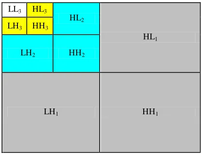
contains the three subbands which are required to reconstruct the image with twice the horizontal and vertical resolution. For example, for K = 3, R0 = {LL3}, R1 = {LH3, HL3, HH3},

R2 = {LH2, HL2, HH2}, and R3 = {LH1, HL1, HH1}, as shown

in Figure (1). This wavelet decomposition is referred to as dyadic or Mallat decomposition [2], [3].

LL3 HL3

HL2

HL1 LH3 HH3

LH2 HH2

LH1 HH1

Fig. 1. an image with 3 (2-D) DWT decomposition levels

Wavelet-based set partitioning image compression techniques such as the SPIHT [4] and the Set Partitioning Embedded bloCK (SPECK) [5] algorithms are the benchmark for the state-of-the-art wavelet-based image compression techniques [6]. These schemes employ some kind of significance testing for sets of pixels, in which the set is tested to determine whether the maximum magnitude in it is above a certain threshold. If the set is significant (SIG), it is partitioned; and if the set is insignificant (ISIG), it is represented by one symbol. The same process is repeated for the SIG sets until all pixels are encoded. The main advantages of these schemes are they have relatively low computational complexity, their performance is comparable to the best -known image coding algorithms , and they generate an embedded compressed bit-stream which can be truncated at

Low Memory Set-Partitioning in Hierarchical

Trees Image Compression Algorithm

Ali Kadhim Al-Janabi

any point while maintaining the best possible quality for the selected bit rate [5], [7]. The embedding property is very interesting feature in heterogeneous networks such as the Internet as users may have different resource capabilities in terms of processing speed, available memory and power. Accordingly, each user can request an image quality t hat fits his need [8]. The price to be paid for these advantages is the high memory requirements as these algorithms use linked list structures to keep track of which sets/pixels need to be tested . At high rates, the lists sizes may be larger than the image size. In addition, the linked list memory management is complex due to the continual process of adding and removing elements to and from these lists. Finally, the size of the lists cannot be pre-allocated because the number of list entries can’t be determined in advance as it depends on the compression bit -rate and on the amount of image details. This problem can be solved by using either dynamic memory allocation or pre -allocating the lists to the maximum size. The former solution slows the algorithm and the latter one increases its memory requirements [9].

Several works that reduced the memory requirements of the set partitioning algorithms are presented in the literature. A reduced memory version of SPIHT algorithm termed No List SPIHT (NLS) is presented in [10]. NLS uses one list and a state table that requires four bits per coefficient. However, NLS still requires about 56% of additional memory with respect to size of the image. In addition, the size of the list and the state table are fixed. This means that NLS needs the same memory regardless of the compression bit-rate. This is a problem for applications that need low bit-rate (quality) compressed images. A low memory SPECK algorithm is presented in [11]. It adopted the method of NLS to reduce the memory of SPECK. Therefore it has exactly the same limitations of NLS. Another low memory algorithm termed Modified SPIHT (MSPIHT) is presented in [12]. It uses a two bit state mark table and a list of size of ¼ the image size to store the maximum value of zerotree set’s coefficients. MSPIHT has lower memory than NLS. However, it merges the sorting and the refinement passes into one pass. This leads to reduce the algorithm’s performance due to violating the embedding principle [7], [13].

In this paper, we propose a new algorithm that is based on SPIHT. The new algorithm termed Single List SPIHT (SLS) makes use of a single list and a two bit state mark table only instead of the three lists that are used by the original SPIHT. In addition, the proposed SLS has simpler memory management because once a pixel is added to the list it will never be removed. This will permit to implement the list as a simple ordered 1-D array that is accessed sequentially in First In First Out (FIFO) manner which is the fastest memory access method [14].

The remainder of the paper is organized as follows: section II gives brief review for the SPIHT algorithm. Section III introduces the new SLS algorithm. Section IV gives an analytical study of the memory requirements of the SPIHT, NLS, MSPIHT and the SLS algorithms. Section V covers the

experimental results of these algorithms. Finally, Section VI gives the concluding remarks of the paper.

II.

SPIHT

The SPIHT algorithm [4] exploits the correlation between the wavelet coefficients that exists across the DWT image subbands (the inter-band correlation) by grouping the related coefficients into trees called Spatial Orientation Trees (SOTs). More specifically, every coefficient at a given resolution level (except the highest level) is related to four coefficients at the next level of similar orientation. The coefficient at the lower level is called the parent, and the four children at the next level are called the offspring and the set of all parent's children at all levels are called the descendent. The SOTs are constructed as follows: the pixels in LLK subband are formed

into groups of 2×2 adjacent pixels. Out of these, the top -left pixel of each group, is not part of any tree, i.e. it has no offspring. Each of the other three pixels has four offspring in groups of 2×2 pixels in subbands LHK, HLK, and HHK

respectively. Then, the pixels in LHk, HLk, and HHk, K ≥ k >

1, are linked with subbands at the next level LHk-1, HLk-1, and

HHk-1 as follows: each pixel at coordinates (i, j) from the LHk,

HLk, and HHk acts as a root for the pixels at coordinates (2i,

2j), (2i+1, 2j), (2i, 2j+1), and (2i+1, 2j+1) in LHk-1, HLk-1 and

HHk-1 respectively. Evidently, the LH1, HL1, and HH1 have no

offspring. Figure (2) depicts part of the SOTs for the first group of 2×2 pixels in a DWT image with 2 decomposition levels.

The SPIHT algorithm makes use of three linked lists, called List of Insignificant Sets (LIS), List of Insignificant Pixels (LIP), and List of Significant Pixels (LSP). In all lists each entry is identified by a coordinate (i, j), which in the LIP and LSP represents individual pixels, and in the LIS represents the roots of the SOTs . In addition to roots coordinates, every entry in LIS has a type field that makes the set of type A or B. A set of type A represents a root for all its descendants (a complete SOT) whereas a set of type B represents a root for all its descendants excluding its direct offspring.

The algorithm consists of four stages: initialization, sorting

pass, refinement pass , and quantization step update. At the initialization stage, it first computes the maximum bit-plane (n) based on the maximum value of the DWT image and it is given by:

⌊

|

| ⌋

where I is the DWT Image, cij is a wavelet coefficient at

location (i, j), and  x  is the nearest integer ≤ x. Then, it initializes the LIP with the coordinates of all the pixels in the lowest resolution level (i.e. LLK subband), the LIS with all the

coordinate of pixels in LLK subband that have offspring as

type A sets, and the LSP as an empty list.

At each bit-plane except the first (the maximum), the encoding consists of two passes: the sorting pass and the refinement pass. Only the sorting pass is made for the first bit -plane. The sorting pass identifies the new SIG coefficients and the refinement pass codes the coefficients that are found SIG at previous passes. For a given bit-plane n, a coefficient cij is

considered SIG with respect to n if

|

|

respect to n if the set contains one or more SIG coefficients; otherwise it is ISIG.

During the sorting pass, the entries in LIP (which represent the (i, j) coordinates of the corresponding pixels) are tested for significance with respect to n. If the pixel is ISIG, a (0) is transmitted to the compressed bit-stream. On the other hand, if the pixel is SIG, a (1) and a sign bit representing the sign of that pixel (e.g., 0 for positive and 1for negative pixel) are transmitted to the bit-stream, and the entry is removed from LIP and added to end of LSP to be refined in the next bit-plane passes. Next, the entries in LIS (which represent the (i, j) coordinates of the roots of the SOTs) are tested. If the entry is of type A, its SOT is tested for significance. If the SOT is ISIG, a (0) is transmitted (i.e., the whole SOT is represented by a single bit). On the other hand, if the SOT is SIG, a (1) is transmitted, and the set’s four offspring are tested as follows: if an offspring is SIG then a (1), and its sign bit are transmitted, and its coordinates are added to the end of LSP. Otherwise (the offspring is ISIG), a (0) is transmitted and its coordinates are added to LIP. Finally, if the set has grandchildren, it is moved to the end of LIS as a type B set. The type B sets are tested for significance as follows: if any of the four offspring of the B set is SIG, a (1) is transmitted, the set is removed from LIS, and its four offspring are added to the end of LIS as type A sets to be tested in the current pass. On the other hand, if the B set has no SIG offspring, a (0) is transmitted and the set remains in LIS to be tested in next bit-plane passes.

In the refinement pass, all entries in the LSP, except those which have been added to it during the current pass, are refined by outputting its nth MSB to the bit-stream. For the quantization step, n is decremented by 1 and the sorting and refinement passes begins again for the next bit-plane.

From this brief description, we can deduce that SPIHT has

the following drawbacks:

 It needs a huge amount of memory due to using the lists. More precisely the LIP and LSP lists which store the (i, j) coordinates of individual pixels dominate the total storage. The maximum number of entries in each list is equal to the number of image pixels. On the other hand, the LIS has less memory requirement because it stores the (i, j) coordinates of the roots of the SOTs. In addition, the roots in the highest level (LH1, HL1, and

HH1 subbands) are not stored because they don't have

descendants. The size of these subbands is 3/4 the image size. Thus the maximum size of LIS is 1/4 the image size. Therefore, the maximum working memory of SPIHT is at least 2.25 times the image size.

 It has complex memory management as the list nodes are added, deleted, or moved from one list to another.  The list sizes can't be pre-allocated. So, it may use either

the slow dynamic memory allocation or initializing lists to the maximum size.

III. THE PROPOSED SINGLE LIST SPIHT (SLS) ALGORIT HM

The proposed SLS overcomes the huge memory requirements and the complex memory management drawbacks of the original SPIHT. The basic idea of the new SLS is based on the fact that the LIP and LSP lists are constructed from the offspring (the four children) of a root that belongs to a SIG SOT. So, instead of storing the offspring in these lists, they can be recomputed in each pass. Evidently, this will increase the algorithms' complexity. On the other hand, the SLS algorithm greatly simplifies the memory management problem (as shown shortly). Consequently, this complexity increment is compensated by the reduced memory management overhead.

The algorithm makes use of a single list termed the List of Root Sets (LRS). Like LIS, LRS stores the (i, j) coordinates of the roots of the SOTs. So LRS has exactly the same size as LIS. However, LRS differs by the following two points:

 Once a set is added to LRS, it will be never removed. Thus LRS can be implemented as a simple 1-D array that is accessed sequentially in First In First Out (FIFO) manner. In contrast, the LIS must be implemented as a linked list that is accessed in random manner dueto the continual process of adding and removing elements to and from it.

 The type field is used differently. A set of type A is untested set or a set that has no SIG SOT whereas a set of type B has one or more SIG SOT. In other words, a set in LRS is initialized as type A and becomes of type B when one of its SOTs becomes SIG.

In addition, SLS replaces the LIP and LSP lists (which dominate the total memory usage) by state mark bits. More specifically, each pixel in LLK is provided by a single status

provided by two status bits termed  to determine the type of the pixel as follows:

  = 0: New ISIG Pixel (NIP). A NIP is an ISIG pixel that is not yet tested. It may belong to the offspring of type A sets in LRS that just become SIG in the current bit-plane pass.

  = 1: Visited ISIG Pixel (VIP). A VIP is a pixel that is tested ISIG in the previous passes. It may belong to the offspring of the sets of type B in LRS (i.e., sets that became SIG in the previous bit-plane passes). It should be noted that the SPIHT store the (i, j) coordinates of these VIPs in the LIP list that are coded in the sorting pass.

  = 2: New SIG Pixel (NSP). A NSP is a pixel that just becomes SIG in the current bit-plane pass.

  = 3: Visited SIG Pixel (VSP). A VSP is a pixel that is tested SIG in the previous passes . It may belong to the offspring of type B sets in LRS (i.e., sets that became SIG in the previous bit-plane passes). It should be noted that the SPIHT store the (i, j) coordinates of these VSP pixels in LSP that are coded in the refinement pass.

The SLS algorithm consists of an initialization stage and several bit-planes coding passes. At the initialization stage, SLS first computes and outputs the maximum bit-plane n. Then it initializes the LRS to the (i, j) coordinates of the pixels in LLK subband that have offspring as type A sets.

The first bit-plane pass starts by coding pixels in LLK

subband. A pixel cij in LLK is coded by testing it for

significance with respect to bit-plane n. If cij is still ISIG, a (0)

is outputted to the bit-stream. On the other hand, if the pixel cij

becomes SIG, a (1) and its sign bit are outputted to the bit-stream and its status bit ij is updated to 1. Next, the sets of

LRS (which are sets of type A) are sequentially processed as follows: the SOT of the set is tested for significance with respect to n. If the SOT is ISIG, a (0) is outputted (i.e., the whole SOT is represented by a single bit). On the other hand, if the SOT is SIG, a (1) is outputted, the set’s type is changed to type B set, and each one of the set’s four offspring (which is an NIP) is tested for significance with respect to n. If it is still ISIG, a (0) is outputted to the bit-stream, and it is marked as a VIP. On the other hand, if the pixel becomes SIG, and (1) and its sign bit are outputted to the bit-stream, and it is marked as a NSP. Finally, if the set has grandchildren, the four offspring are added to the end of LRS as type A sets to be coded in the current bit-plane pass.

Each one of the next bit-plane coding passes starts by coding the pixels in LLK. These pixels are coded according to

their types depending on the value of their status bits . If ij =

0, the pixel cij is ISIG, it is coded in the same way as was done

in the first pass, and if ij = 1 (the pixel is a SIG), it is refined

by outputting its nth bit to the bit-stream. Notice that the

sorting and refinement passes are merged for the pixels in LLK

subband which may reduce the Peak Signal to Noise Ratio

(PSNR) performance of the algorithm due to not preserving information ordering. However, since the size of LLK is small

as compared to the size of the whole image, the reduction is very small.

Next, the LRS list is scanned two times. In the first scan, only the sets of type B are processed by computing its four offspring. A type B set may contain the VIPs and pixel that are found SIG in the previous passes but that are still marked as (NSPs). A NSP is marked as VSP in order to refine it later in the second LRS scan pass. On the other hand, if the pixel is a VIP, it is coded exactly in the same way as coding a NIP. Notice that this step is equivalent to coding the pixels in the list LIP during the sorting pass in the original SPIHT. This means that both algorithms code the VIPs in the same order. Therefore, SLS has the same embedding properties as SPIHT.

In the second LRS scan pass , all the sets in LRS are processed. If the set is of type A, it is processed exactly in the same way as was done in the first pass . On the other hand, if the set is of type B, only the VSPs of the set’s four offspring are refined by outputting their nth bit to the bit-stream. Finally

n is decremented by 1 to start a new bit-plane coding pass.

It should be noted that coding the VSPs of the type B sets in the second LRS scan pass is equivalent to refining the pixels in the list LSP during the refinement pass in the original SPIHT algorithm. This means that the proposed SLS algorithm merges the NIPs and the VSPs. In contrast, the MSPIHT algorithm [12] merges the VIPs and VSPs by merging the sorting and the refinement passes . It can be shown that the VIPs have highest effect on distortion reduction than the NIPs and VSPs (which have nearly the same distortion reduction effect) [7], [13]. Consequently, merging the VIPs and VSPs as done in [12] may result in PSNR reduction, whereas merging the NIPs and the VSPs slightly enhances the PSNR of the SLS algorithm (as will be shown next).

IV. MEMORY AND COMPLEXIT Y ANALYSIS

In this section we will compare the memory requirements of the auxiliary list(s) in the proposed SLS algorithm to that of SPIHT, NLS and MSPIHT algorithms. In addition, we will study the effects of the memory reduction on the complexity of the proposed SLS algorithms. Let:

I: an image of size M × N pixels.

NLIP: number of entries in LIP.

NLSP: number of entries in LSP.

NLIS: number of entries in LIS.

b =



log

(M)



+



log

(N)



(3)

Then total memory required in SPIHT (in bits).

M

= b (N

+ N

+ N

) (4)

In the worst case,

N

= N

= M × N

N

= (M × N) / 4.

Thus the maximum working memory requirement in SPIHT is [11]:

(

)

(5)

The memory requirement of NLS and MSPIHT are fixed and are given by [12]:

(

)

(6)

(

)

(7)

Where W is the number of bits used to store the wavelet coefficient (e.g., 16 bits)

The proposed SLS algorithm uses only the list LRS, a single status bit for pixels in LLk subband, and two status bits for

pixels in the other subbands. However, as LLK has small size

and in order to simplify the analysis , all pixels are assumed to have two status bits. So, the maximum working memory requirement in SLS is:

(

)

(8)

For instance, for grayscale image of size 512×512 pixels, b = 2 × log2(512) = 18 bits and W = 16 bits . Hence the total

memory required by the SPIHT, NLS, MSPIHT, and SLS are:

₍

)

= 1327104 bytes = 1296 KB

{ ( ) }

= 294912 bytes = 288 KB

{ ( ) }

= 172032 bytes = 168 KB

{ ( ) }

= 212992 bytes = 208 KB

The memory ratio between the algorithms is

= 6.23:1.38:0.8:1

It can be seen that the proposed algorithm has reduced the memory requirement by factors of 6.23, and 1.38 in comparisons to SPIHT, and NLS respectively. The other advantage of SLS over NLS is that the working memory of NLS is fixed whereas the working memory of SLS is variable and it depends on compression bit-rate. On the other hand, although the SLS has slightly higher memory requirement than MSPIHT, SLS has the advantage of preserving information ordering while the MSPIHT don’t have this characteristic because as mentioned before, it merges the sorting and refinement passes into one pass which leads to reduce the algorithm’s performance [13].

The second interesting feature of SLS over the other algorithms is the simple memory management. As shown, the LRS in SLS is easily implemented as 1-D array that is accessed in FIFO manner because the new nodes are added to the end of the array. In contrast, in SPIHT, the LIP and LIS must be implemented as linked lists that are accessed randomly due to the continued process of nodes removing and insertion (i.e., the added nodes must be put in the same position of the removed ones). It should be noted that adding an item to the end of an array is very simple process that can be performed on fly because it requires a constant time regardless of the size of the array. On the other hand, the time needed to removing and insertion nodes randomly from and to a linked list increases with the size of the list [14]. It is worth to noting that the reduced complexity of SPIHT is mainly due to using the LIP and LSP lists as only the elements in these lists (VIPs and VSPs) are tested and coded in the individual bit-plane passes. On the other hand, the SLS needs to re-compute the offspring in each bit-plane pass in order to code the VIPs and VSPs. Evidently this process increases complexity of the SLS algorithm. From this analysis, we can deduce that the SLS and SPIHT have about the same complexity because the increased complexity of re-computing the offspring is compensated by the complexity reduction of the list management. The simulation results of the algorithms presented in the next section will demonstrate this analysis.

V. EXPERIMENT AL RESULT S

Noise Ratio (PSNR) versus the compression bit-rate (the average number of bits per pixel (bpp) for the compressed image). PSNR is given by:

(9)

Where max_pix is the maximum value of the pixel and MSE is Mean-Squared Error between the original and the reconstructed images defined as:

∑

∑

[

]

10)

where Io is the original image, Ir is the reconstructed image, and MN is the image size (number of pixels). Evidently, smaller MSE and larger PSNR values correspond to lower levels of distortion.

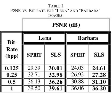
Table (1) shows the PSNR versus bit-rate for the SPIHT and the proposed SLS algorithms. The results of SPIHT are obtained by implementing the Public License Matlab program presented by Dr. Mustafa Sakalli and Dr. William A. Pearlman [15] using the same test images. The table clearly depicts that SLS has slightly better PSNR than SPIHT for all bit-rates for the two images . These results demonstrate that the merging the bits of the New ISIG Pixels (NIPs) and the Visited SIG pixels (VSPs) by the adopted coding method increases the algorithms' efficiency. This feature is unique to the proposed algorithm because the other reduced memory algorithms have lower PSNR than SPIHT [7], [10], [13].

TABLE I

PSNR VS.BIT-RATE FOR "LENA" AND "BARBARA"

IMAGES

PSNR (dB)

Bit

-Rate

(bpp)

Lena

Barbara

SPIHT

SLS

SLS

0.125

29.39

30.01

24.03

24.61

0.25

32.71

32.98

26.92

27.28

0.5

36.13

36.26

30.88

31.10

1

39.50

39.61

36.06

36.20

As mentioned before, the complexity of the SLS algorithm is very close to that of the original SPIHT due to the simplification in memory management. In order to demonstrate this, the SLS and SPIHT are implemented under the same environments (using C++ and the same computer). Table (2) represents the complexity of the SLS and SPIHT represented by the processing time (measured in milliseconds (msec)) required by the algorithm to encode and to decode the "Lena" image at several bit-rates. The processing time of the

2-D DWT is not computed since it is the same for both algorithms. As it can be shown, the proposed SLS has a very slight increment in the processing time of coding and decoding with respect to the original SPIHT. These results verify our complexity analysis presented in the previous section.

TABLE II

PROCESSING TIME VS.BIT-RATE FOR "LENA" IMAGE

Coding time

(msec)

Decoding time

(msec)

Bit

-Rate

(bpp)

SPIHT

SLS

SLS

0.125

15

16

5

7

0.25

20

22

10

11

0.5

26

28

20

22

1

31

32

25

26

VI. CONCLUSION

In this paper, we developed a low memory version of SPIHT algorithm. The proposed SLS make use of a single list with size of ¼ the image size. In addition it replaces the LSP and LIP lists (which have sizes of about 2 times the image size) by 2 bits state mark bitmap. The theoretical analysis and experimental results clearly showed that the proposed SLS algorithm has better PSNR than SPIHT and it has nearly the same coding time as the SPIHT. This means that we reduced the memory requirements by about six times and enhanced the performance of SPIHT without affecting its simplicity and without paying additional overhead cost. The reduced memory requirement and management of the SLS algorithm makes it very suitable for memory constrained portable hand held devices . Furthermore, as the SPIHT is extended to Multispectral [16], and to 3-D image compression systems [17], the current work can also be very useful for these image compression applications benefiting from its reduced memory and simplicity.

REFERENCES

[1] Shi Y. Q. and Sun H., “Image and Vide o C ompre ssion for Multimedia Engineering: Fundame ntals, Algorithms, and

Standards,” 1st _{edition, CRC Press, 2000.}

[2] Salomon D., “Data Compression: the C omple te Re fe re nce,” third edition, Springer, 2004.

[3] Lawson S. and Zhu J., “Image Compression using Wavelets and JPEG2000: a Tutorial,” IEE Electronic & Communication Journal, pp. 112-121, June 2002.

[4] A. Said and W. A. Pearlman, “A New, Fast, and Efficient Image C ode c Based On Set Partitioning in Hierarchical Tre es,” IEEE T ransactions on Circuits and Systems for Video T echnology, Vol. 6, No. 3, pp. 243-250, June 1996.

Communications and Image Processing, Proceedings of SPIE, Vol. 3653, pp. 294-305, January 1999.

[6] Ranjan, K. et al, "Listless Block-tree Set Partitioning Algorithm for Ve ry Low Bit-rate Embe dde d Image C ompre ssion," Elsevier, International Journal of Electronics and Communications, pp 985-995, 2012.

[7] Rabbani M. and Joshi R., “An Overview of the JPEG 2000 Still Image C ompre ssion Standard,” Signal Processing: Image Communication, Vol. 17, No. 1, pp. 3 -48, Jan. 2002. [8] T aubman D., “Successive Refinement of Vide o: Fundame ntal

Issues, Past Efforts and New Directions,” Int. Symp. on Visual Communication and Image Processing, Vol. 5150, pp. 791-805, July 2003.

[9] Chrysafis C. et al, “SBHP-A Low C omplexity Wavelet C ode r,” IEEE Int. Conf. Acoust., Speech and Sig. Proc. (ICASSP2000), vol. 4, pp. 2035-2038, June 2000.

[10] F. W. Wheeler and W. A. Pearlman “SPIHT Image Compression without Lists,” Proceedings of IEEE International Conference on Acoustics, Speech and Signal Processing, ICASSP 2000, vol. 4, pp. 2047–2050, June 2000.

[11] Latte, M. V., N. H. Ayachit, et al., "Reduce d Me mory Listle ss SPEC K Image Compression," IEEE Digital Signal Processing Vol. 16 No. (6), pp 817-824, 2006.

[12] Jianjum, W. and Bo Liu, "Modifie d SPIHT Base d Image C ompression for Hardware Implementation," IEEE Computer Society, second International Workshop on Computer Science and Engineering, pp 572-576, 2009.

[13] Ordentlich E. et al, “A Low-Complexity Modeling Approach for Embe dde d C oding of Wavelet Coefficients,” Proc. IEEE Data Compression Conf. (Snowbird), pp. 408 -417, March 1998. [14] Berman A. M., “Data Structure s via C ++: O bje cts by

Evolution,” OXFORD University Press, 1st

edition, 1997. [15] http://www.cipr.rpi.edu/research/SPIHT

[16] Zhong Cuixiang, Huang Minghe, "Furthe r Improve me nt of SPIHT for Multispe ctral Image C ompre ssion," IEEE International Forum on Information Technology and Applications, pp 337-340, 2010.