ISSN : 2230-7109 (Online) | ISSN : 2230-9543 (Print)
Analysing Resolution Parameters of Different Direction
of Arrival Estimation Algorithm for
Un-correlated Environment
1
Dhusar Kumar Mondal,
2Aritra Mondal,
3Pranoy Das,
4Chayan Seth,
5B N Biswas
1Dept. of ECE, SKFGI, Mankundu, Hooghly, WB, India
Abstract
High resolution Direction Of Arrival (DOA) estimation algorithm enhance the performance of smart antenna system, the key technology to solve spectrum scarcity problem. This paper presents the detection capability of conventional Bartlett and Capon algorithm and subspace based MUSIC algorithm. A large no of simulation study is carried out in this paper to investigate the resolution of different DOA algorithms like Bartlett method, Capon Method and MUSIC in an un-correlated sources environment based on uniform linear array. The work come out with the plot of resolution curve of above three algorithm with variation of different design parameters for selection and practical implementation of any algorithm.
Keywords
SDMA, Resolution Curve, MUSIC Algorithm, DOA Estimation, Un-correlated Sources
I. Introduction
The high demand on the usage of the wireless communication
system calls for higher traffic handling capacities. The system
capacity can be improved either increasing its frequency bandwidth by allocating new portion of frequency spectrum to wireless services. But since the electromagnetic spectrum is a limited resource, it is not easy to get new spectrum allocation without the international allocation on the global level. Instead
we can increase spectrum efficiency by increasing the frequency
reuse factor within the same geographical area which is a very challenging task. Because it caused co-channel interference by which the security of data as well as SNR will be decreases. With the advances in digital Communication techniques, the spectrum
efficiency can be improved by various multiple access techniques
which allow mobile users to access whole bandwidth resource and hence improves the system’s capacity.
Fig. 1: Concept of SDMA
So a new multiple access technique is introduce known as Space Division Multiple Access (SDMA) additionally introducing the dimension space with the existing technique like Frequency Division Multiple Access (FDMA), Time Division Multiple Access (TDMA) and Code Division Multiple Access (CDMA).
This Technique is implemented with the help of Smart Antenna [1-2]. The Smart Antenna System (SAS) employs the array antenna technology and the digital signal processing which enables it to form a beam to a desired direction by suppressing other direction propagation components as in the case of isotropic antenna. In this way, Signal-to-Interference Ratio (SNR) improves by focussing the beam towards the desired user and forming nulls towards the interferers. Ultimately the performance of SAS greatly depends on the performance on DOA estimation.
In the paper the performance of MUSIC algorithm and its resolution curve are investigated in different parametric situation with MATLAB as a simulation tool. The performance of these algorithms is analysed by considering parameters like number of array elements, number of snapshots, signal to noise ratio which results in optimum array design for Smart Antenna system.
II. Basic Theory
Let us first assume that k uncorrelated sources transmit signals to
an n-element uniform linear array with interelement distance d. To study the resolution of the DOA Algorithm we assumed, (1) all the sources are completely un-correlated to each other and the signals come in antenna array in direct path (2) antenna elements in this array are isotropic and non-dispersive in nature and mutual coupling effect is neglected to reduce the mathematical complexity (3) noise is AWGN with zero mean.
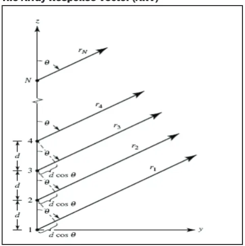
The concepts of the ‘array response vector’and the ‘signal auto-covariance matrix’ is an urgent need to implement any of DOA estimation algorithm. The received signal auto-covariance matrix Rxx and the desired signal auto-covariance matrix Rss will be utilised to calculate spatial spectrum [3].
The Array Response Vector (ARV)
(1)
Assuming that an antenna array along z axis is composed of identical isotropic elements and each element receives a
time-delayed version of the same plane wave with wavelength λ. In other words, each element receives a phase-shifted (ψ) version
of the signal.
The ARV is a combination of the steering vector and the response of each individual element to the incident wave. The ARV of of kth source is [4]
(2)
where n is the total number of antenna elements in the array and
θk is the elevation angle of kth source. ARV simplifies to the SV
A(θ):
A(θ)=[a(θ1), a(θ2), a(θ3),….., a(θk)] (3)
B. Received Signal Model
Under this model, the received signals can be expressed as a superposition of signals from all the sources and linearly added noise represented by the following equation:
(4)
Where ,σn2 be the noise power, I be the identity matrix
and the a(θk) is the array factor.
X(t) is the complex baseband equivalent received signal vector at the antenna array
( )
t
[
x
1(
t
),
x
2(
t
),
x
(
t
)
]
X
=
N (5)A single observation x(t) from the array is often referred to as a snapshot. Now in matrix notation x(t) can be written as follows:
(6)
C. Signal Auto-covariance Matrices
In reality, the expected value cannot be obtained exactly, since an
infinite time interval is necessary to estimates. Hence, the average of sufficiently enough number of data or snapshots (M) over a finite interval must be used in practical implementations.[5,6] The
received signal auto-covariance matrix Rxx and the desired signal auto-covariance matrix Rss are given by the following equation:
(7)
The physical signification of Rxxis that it is nothing but the signal
received by the antenna array. After getting all the matrices the directions of arrival of the sources are determined by the DOA
algorithm. Basically non-parametric DOA estimation are classified
as:
Conventional DOA Estimation Method. Subspace DOA Estimation Method.
III. Conventional DOA Estimation
The conventional methods are the earliest methods of DOA Estimation which are based on the incoming signal scanning the
beam of the radiation pattern, and surveying the space of signals
above a certain threshold. Two methods are usually classified as
conventional methods,
The Conventional Beamforming Method/Bartlett method.
•
Capon’s minimum Variance Method.
•
A. Conventional Beamforming Method / Bartlett Method
The Conventional Beamforming Method (CBF) is the earliest method of spatial analysis and it is also referred to as the Bartlett method. The idea is to scan across the angular region of interest in discrete steps are implemented here and whichever direction produces the largest output SNR then it is the estimate of the
desired signal’s direction. More specifically, as the look direction θ is varied incrementally across the space of access. The spatial
spectrum of the beam former is measured by the following equation:
(8)
The estimate of the DOA is the angle θ that corresponds to the
peak value of the output power spectrum. The poor resolution is
a significant limitation of this method.
B. Capon’s Minimum Variance Method
It is also known as the Minimum Variance Distortion less Look (MVDL). The MVDL is an attempt to overcome the poor resolution problem associated with the Bartlett method and it
results a significant improvement of conventional beam forming
method. In this method, the output power is minimized with the constraint that the gain in the desired direction remains same. Solving this constraint optimization problem for the weight vector we obtain the Capon’s Spatial Spectrum:
(9)
(10)
The MVDL only requires an additional matrix inversion compared to the CBF and exhibits greater resolution in most cases.
IV. Subspace Based DOA Estimation
The other group of DOA estimation algorithms are called the subspace methods. The received signal space can be separated into two subspace like as:
The signal subspace
•
The noise subspace
•
The signal subspace is the subspace spanned by the columns of
A(θ) and the subspace orthogonal to the signal subspace is known as the noise subspace. MUSIC (MUltiple SIgnal Classification)
ISSN : 2230-7109 (Online) | ISSN : 2230-9543 (Print)
A. The MUSIC Algorithm
The popularity of the MUSIC algorithm is very large due to its generality. However, this generality is accompanied with the expense that the array response must be known for all possible combinations of source parameters; i.e., the response must be either measured (calibrated) and stored. It is applicable to any arbitrary
arrays but known configuration and response and it can be used to
estimate multiple parameters per source (e.g. azimuth, elevation, range, polarization, etc.). MUSIC requires apriori knowledge of the second-order spatial statistics of the background noise and
interference field. This method involves a correlation analysis of
the array signals followed by Eigen decomposition method and signal / noise space information.
B. MUSIC Spatial Spectrum
Inside the algorithm, the subspace estimation step is typically achieved by Eigen decomposition of the auto-covariance matrix of the received data Rxx. Furthermore, it can be easily shown that Rxx can be written in the following form:
where E = [e1, e2, . ., eN], Es= [e1, e2, . ., eK], En = [eK+1, eK+2, . ., eN], Λ= diag{λ1, λ2, . ., λN}, Λs= diag {λ1, λ2, . . ., λK}, Λn= diag {λK+1, λK+2, . . , λN}, and Λs = Λs− σn2I.
Once the subspaces are determined, the DOAs of the desired signals can be estimated by calculating the MUSIC spatial spectrum overthe region of interest [9]
(11)
Due to imperfections in deriving Rxx, the noise subspace Eigen
values will not be exactly equal to σn2. They can be distinguished
from the signal subspace eigen values. Although the MUSIC
provides the maximum detection efficiency, they are achieved at
a considerable cost in computation and storage and in either low SNR scenarios or closely spaced sources (less than 5 degrees) then multiple peaks observed in the measurements and MUSIC’s performance reduces dramatically [10-11].
V. Simulation Results
Common Parameters : No. of Sources (S) = 3; No. of Snapshot (M) = 100; Sources Angle= -30, 0, 30; SNR = 10 dB
Simulation-1:
From the fig.4 and 5 it is seen that for Bartlett and Capon the
3dB beam width gradually decreasing with respect to the no. of elements. That means we cannot operate, these two algorithms for lower no. of elements. But for MUSIC as 3dB beam width is very narrow, slightly decreasing with respect to the no. of elements, gives reasonable level of resolution for lower no. of array elements also. MUSIC has very less amount of dependency upon N. For Bartlett and Capon can not be implemented for small array size of 5 or less.
5 6 7 8 9 10 11 12
0 2 4 6 8 10 12 14 16 18 20
No. of Antenna E lements -->
3dB Beam Width (degree)-->
R es olution Curve of Half-power B eam W idth for different DOA
CB F CAP ON MUS IC
Fig. 4: Resolution curve (3dB Beamwidth vs no. of elements).
4 5 6 7 8 9 10 11 12
-25 -20 -15 -10 -5 0
No. of Antenna E lements -->
Minimum value of P(theta) between peak (dB)-->
R es olution Curve of Minimum value of P (theta) for different DOA
CB F CAP ON MUS IC
Fig. 5: Resolution curve (Minimum value of Pseudospectra vs no. of elements)
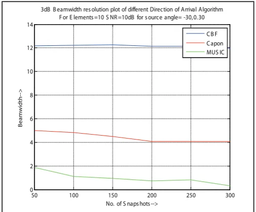
Simulation-2:
Parameters: No. of Elements (N) = 10;
50 100 150 200 250 300
0 2 4 6 8 10 12 14
No. of S naps hots -->
Beamwidth-->
3dB B eamwidth res olution plot of different Direction of Arrival Algorithm For E lements =10 S NR =10dB for s ource angle= -30,0.30
CB F Capon MUS IC
50 100 150 200 250 300 -30
-28 -26 -24 -22 -20 -18 -16 -14 -12
No. of S naps hots -->
Spatial Spectrum P(theta)-->
Minimum value of P (theta) res olution plot of different Direction of Arrival Algorithm F or E lements =10 S NR =10dB for s ource angle= -30,0.30
CB F Capon MUS IC
Fig. 7: Resolution Curve (Minimum Value of Pseudospectra vs Varying No. of Snapshots)
Decrease in value of Pseudospectra for MUSIC with increase in no. of snapshots indicates the improvement in performance where as Bartlett and Capon’s methods do not indicates any appreciable improvement.
Simulation-3
Parameters: No. of Sources (S) = 4; No. of Elements (N) = 10; Sources Angle = (-60,-20,10,50);
10 15 20 25 30 35 40 45 50 55 60 -80
-70 -60 -50 -40 -30 -20
S NR (dB )->
Peak to Minima differance of Spacial Spectrum (dB)->
P s eudo S pectra of MUS IC Algorithm F or ULA of S ources = -20,-60,10,50. Antenna Array E lements = 10 S naps hot= 100
Fig. 8: Resolution Curve for MUSIC (Minimum Value of Pseudospectra vs SNR).
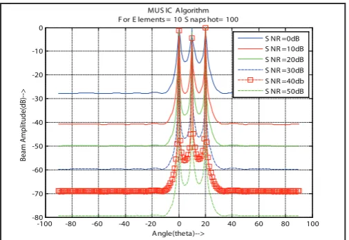
Simulation-4
Parameters: Sources Angle= (0, 10, 20);
-100 -80 -60 -40 -20 0 20 40 60 80 100
-80 -70 -60 -50 -40 -30 -20 -10 0
Angle(theta)-->
Beam Amplitude(dB)-->
MUS IC Algorithm F or E lements = 10 S naps hot= 100
S NR =0dB S NR =10dB S NR =20dB S NR =30dB S NR =40db S NR =50dB
Fig. 9: Performance of MUSIC Algorithm by Varying SNR
Simulation-5
Parameters: SNR= 40dB; Angle of sources= 0o, 3o, 6o.
-100 -80 -60 -40 -20 0 20 40 60 80 100
-80 -70 -60 -50 -40 -30 -20 -10 0
Angle(theta)-->
Beam Amplitude(dB)-->
MUS IC Algorithm
F or E lements = 10 S naps hot= 100 S NR = 40dB
Fig. 10: Detection Performance of MUSIC Algorithm for 30 Differences
From the above resolution curve it is seen that for increasing SNR the minimum value of Pseudo Spectra is decreasing very sharply. That means for higher value of SNR the MUSIC can detect two consecutive sources which angular distance with respect to antenna is very small (near to 10o) and in 40dB SNR MUSIC can
detect sources up to 3o deference.
VI. Conclusion
Uniform Linear Array with any DOA estimation algorithm can only detect the azimuth angle or elevation angle depending upon orientation of array. An in depth analysis of three algorithm MUSIC, Bartlett, Capon studied in this paper, shows there variation in performance with different design and implementation parameters like No of elements in array, No of snapshots taken for one psudospectra calculation, SNR etc. Though MUSIC seems to be the excellent one, among these three, but other two also can be implemented where low resolution is tolerable, as cost of implementation is attractive. Different design and implementation parameter can easily be selected for practical application from the entire curves plotted here depending upon the algorithm choose.
References
[1] Dhusar Kumar Mondal,"Studies of Different Direction of Arrival (DOA) Estimation Algorithm for Smart Antenna in Wireless Communication”, International Journal of Electronics & Communication,Vol. 4, Issue-SPL-2, Jan-Mar2013.
[2] Dhusar Kumar Mondal,"Study of Spectral Music Direction of Arrival Estimation Algorithm of Smart Antenna Using Half-Wavelength Dipole Uniform Linear Array”, International Journal of Electronics & Communication, Vol. 5, Issue-SPL-2, Jan-Mar 2014.
[3] Constantine A. Balanis, Panayiotis I. Ioannides, “Introduction to Smart Antennas”, Synthesis Lecture on Antennas#5. 2007 Morgan & Claypool Publishers.
[4] Gaurav Chaitanya, Ankit Jain, Nitin Jain,"Performance Analysis of Direction of Arrival Estimation Algorithms for Smart Antenna for Mobile Communication Systems”,
ISSN : 2230-7109 (Online) | ISSN : 2230-9543 (Print)
Vol. 3, Issue 7, July-2012.
[5] RahmatSanudin, Nurul H. Noordin, Ahmed O. El-Rayis, NakulHaridas, Ahmet T. Erdogan, TughrulArslan,“Analysis of DOA Estimation for Directional and Isotropic Antenna Arrays”, 2011 Loughborough Antennas & Propagation Conference 14-15 November 2011, Loughborough, UK. [6] R. Schmidt,“Multiple emitter location and signal parameter
estimation”, IEEE Trans. Antennas Propagation, Vol. 34, No. 3, pp. 276–280, Mar. 1986.
[7] A. Swindlehurst,“Alternative algorithm for maximum likelihood DOA estimation and detection”, IEE Proc. Radar Sonar Navig., Vol. 141, No. 6, pp. 293–299, Dec. 1994. [8] C. P. Mathews, M. D. Zoltowski,“Eigen-structure techniques
for 2-D angleof arrival with uniform circular arrays”, IEEE Trans. Signal Process., Vol. 42, No. 9,pp. 2395–2407, Sept. 1994.
[9] Tanuja S. Dhope(Shendkar),"Application of MUSIC, ESPRIT and ROOT MUSIC in DOA Estimation”, World Journal of Science and Technology 2011, 1(8), pp. 20-25. [Online] Available: http://www.worldjournalofscience.com, [10] Frank Gross,"Smart Antennas for Wireless Communications
with MATLAB", McGraw Hill Publication, 2005.