Analysis Of Reaction Diffusion Problems Using
Differential Quadrature Method
Mohamed Salah, R.M. Amer and M.S.Matbuly
Faculty of Engineering, Zagazig University, Zagazig, 44519, Zagazig, Egypt.
Abstract-- In this paper, a hybrid technique of differential
quadrature method and Runge-Kutta fourth order method is employed to analyze reaction-diffusion problems. The obtained results are compared with the available analytical ones. Further, a parametric study is introduced to investigate the influence of reaction and diffusion characteristics on behavior of the obtained results.
Index Term-- Reaction-diffusion, Differential Quadrature,
Runge-Kutta.
1. INTRODUCTION
Reaction-diffusion problems frequently arise in engineering, chemical, medical and biological systems. Thermal wave propagation, Fisher and FitzHugh-Nagumo are some models for such problems. Thermal wave physics play an ever-increasing role in the study of material parameters. It has been employed in optical investigations of solids, liquids, and gases with photo-acoustic and thermal lens spectroscopy. Thermal waves have also been used to analyze the thermal and thermodynamic properties of materials and for imaging thermal and material features within a solid sample [1]. Fisher model plays an important role in the spatial spread of gene in population [2]. FitzHugh-Nagumo model can be applied to investigate behavior of heart, excitable cells and muscles [3].
Reaction–diffusion problems have been extensively solved using various techniques. Due to the nonlinearity and complexity of such problems, only limited cases can analytically be solved [4-7]. Yan applied the projective Riccati equation method to solve Schrodinger equation in nonlinear optical fibers [4]. Then Mei, Zhang and Jiang employed the same method to get the exact solutions for some reaction-diffusion problems [5]. Abdusalam applied a factorization technique to find exact traveling wave solutions [6]. Zhaosheng employed Lie technique to solve fisher model in terms of elliptic functions [7]. Literature on the numerical solution of reaction–diffusion equations is sparse; David, Curtis and John introduced time integration methods to solve thermal wave propagation [8]. Marcus applied Finite difference method to study the dynamics of predator–prey interactions [9].As well as, Chen et al. employed the finite element method to solve advective reaction-diffusion equations [10]. Then Christos et al. applied also the same method to solve the problem with boundary layers [11]. Recently differential quadrature method has been efficiently employed in a variety of engineering problems [12].Meral and Sezgin used this method and finite
difference method with a relaxation parameter to solve nonlinear reaction-diffusion equation in one and two dimensions [13]. Moreover, Meral applied differential quadrature method and implicit Euler method to solve density dependent nonlinear reaction-diffusion equation [14]. Wu and Liu have been introduced the generalization of the differential quadrature method to solve linear and non linear differential equations [15].
In spite of all these efforts, analysis of Reaction– diffusion problems is still of significant interests. This research employs a hybrid technique of differential quadrature method (DQM) and Runge-Kutta fourth order method (RK4) for solving reaction-diffusion problems. The obtained results are compared with the previous analytical ones. Furthermore, a parametric study is introduced to investigate the effect of reaction and diffusion parameters on behavior of the obtained results.
2. NUMERICAL PROCEDURE
The main strategy is to employ DQM to reduce the problem to a system of ordinary differential equations then to apply RK4 to solve the reduced system as follows:
2.1. Thermal wave propagation
Propagation of thermal waves through a rectangular plate, is governed by [16]:
2 2
2 0
2 2 2( ) , t 0, (0,0) (x, y) (a, b)
U U U
U U U
t x y
(1)
Where: U is a temperature, α and β are diffusion parameters in direction of x and y, respectively, γ and δ are reaction parameters, a and b are plate dimensions in direction of x and y, respectively and U0 is a maximum temperature of the system.
Along the external boundaries, the temperatures can be described as:
1 ( , , ) 1 1( , )
(0, , )
U
a U o y t b f y t
y t x
(2-a)
2 ( , , ) 2 2( , )
( , , )
U
a U a y t b f y t
a y t x
3 ( ,0, ) 3 3( , )
( ,0, )
U
a U x t b f x t
x t y (2-c)
4 ( , , ) 4 4( , )
( , , )
U
a U x b t b f x t
x b t y
(2-d)
Where , and ,( 1,4),
i i i
a b f i are known functions.
The initial temperature may be described as:
U x y( , ,0)g x y( , ) (3) where g (x, y) is a known function.
Solution of Eqs.(1), (2) and (3) can be obtained as follows: 1- Discretize the spatial domain using
Chebyshev-Gauss-Lobatto grid points[12], such as:
( 1)
1 cos , i 1, 2, , N
2 1 i a i x N (4- a) ( 1)
1 cos , 1, 2, , M
2 1 j b j y j M (4-b)
2- Apply the method of differential quadrature in terms of nodal temperature, such that:
1
(
,
, )
(
,
, )
N x
ik k j
i j k
U
A U x
y
t
x
y
t
x
(5-a)1
( , , ) ( , , )
M y
jl i l
i j l
U
A U x y t x y t
y
(5-b) 2 2 1 ( , , ) ( , , ) N xik k j
i j k
U
B U x y t
x y t
x
(5-c) 2 2 1 ( , , ) ( , , ) M yjl i l
i j l
U
B U x y t x y t
y
(5-d) Where p ijA and Bijp , (p = x, y) are the first and second order weighting coefficients with respect to p [12].
3- On sustainable substitution from Eqs. (5) into (1), one can reduce the problem to the following system of ordinary differential equations as:
( , , ), ( , , ), , (1 1 2 1 , , ) ,
( ,i j, ) ij N M
dU
q U x y t U x y t U x y t
x y t
dt
Or simply
11 21
( , , , , ), i 1, N and j 1,M.
( i, j, ) ij NM
dU
q U U U t
x y t
dt
(6) Where 2 0 2 1 1 ( , , ) ( , , ) ( ) ,
i 1, N and j 1, M.
N M
x y
ij ik k j jl i l ij ij
k l
q B U x y t B U x y t U U U
(7)4- Update the temperature using RK4 such that [17]:
0 0 1 2 3 4
1
( , , ) ( , , ) 2 2 ,
6
ij ij ij ij
i j i j
U x y t t U x y t H H H H
(8)
Where
1 ( 11, 21, , , )0
ij
ij NM
H tq U U U t , (9-a)
11 21
1 1 1
2 ( 11 , 21 , , , 0 )
2 2 2 2
NM ij
ij NM
H H H t
H tq U U U t (9-b)
11 21
2 2 2
3 ( 11 , 21 , , ,0 )
2 2 2 2
NM ij
ij NM
H H H t
H tq U U U t (9-c)
11 21
4 ( 11 3 , 21 3 , , 3 , 0 )
ij NM
ij NM
H tq U H U H U H t t
(9-d) Where
1 0 2 1 P P 1
t
t
t
t
t
t
t
2.2.Fisher model
This model suggests that population density is governed by [18]:
2
0
2 ( ), t 0, 0 x a
U U
D U U U
t x
(10)
Where: U(x, t) is the population density, t and x are time and location respectively,U0 is a maximum population density, γ is
the reaction factor defining the migration rate and D is the diffusion coefficient defining the reproduction rate.
The boundary and initial conditions of such model may be also described as:
1 (0, ) 1 1( )
(0, )
U
a U t b f t
t x (11-a)
2 ( , ) 2 2( )
( , ) U
a U a t b f t
a t x (11-b)
Where
,
and
,(
1, 2),
i i i
a b
f
i
are known functions.The initial temperature can be described as:
( ,0) ( )
U x g x
Where g (x) is a known function.
The proposed technique can be applied to reduce Eqs. (10), (11) and (12) to the following system of ODEs:
(x ,t) (x ,t) 0 (x ,t) 1
, i 1,2, , N
i i i
N i
ij j
dU
D B U U U U
dt
(13)
Where Bij, (i, j = 1,N) are previously defined through Eqs.(5).
Equations (13) can be also solved using Runge-Kutta fourth order method as previously explained in thermal wave model.
2.3.FitzHugh-Nagumo model
This model suggests that cardiac potential is governed by [18]:
2
2 ( )( 1), t 0, 0 x a,0 1
U U
D U U U
t x
(14)
Where: U (x, t) is the cardiac potential at position x and time t,
represent the threshold for excitation, D is the diffusion coefficient and γ is rate parameter of reaction term.Potential along external boundaries can be described as:
1 ( , ) 1 1( )
(0, )
U
a U o t b f t
t x
(15 – a)
2 ( , ) 2 2( )
( , )
U
a U a t b f t
a t x
(15– b)
Where
,
and
,(
1, 2),
i i i
a b
f
i
are known functions.The initial potential may be also described as:
( ,0) ( ),
U x g x (16)
where g (x) is a known function.
The method of differential quadrature can be applied to reduce Eqs. (14-16) to the following system of ODEs:
(x ,t) (x ,t) (x ,t) (x ,t)
1
( )( 1) , i 1, 2, , N
i i i i
N i
ij j dU
D B U U U U
dt
(17)
Where Bij, (i, j = 1, N) is previously defined with thermal
model.
Runge-Kutta method can be also employed to solve Eqs.(17) as in the previous models.
3. NUMERICAL RESULTS
To ensure the efficiency of the proposed technique (DQM + RK4), the three models are solved and compared with the available analytical solution [16,18].Furthermore, a parametric study is introduced to investigate the effects of different reaction and diffusion parameters on the obtained results.
3.1. Results for thermal wave propagation
Consider a one-dimensional problem of thermal wave propagation (along x-direction:
1 2 0 1, 2 8, 3 4 1 2 3 4 3 4 0
a a U a a b b b b f f
).
While 1
2
1 1
( ) 1 tanh 2 t , ( ) 1 tanh(1 2 ) ,
2 2
1
g(x) (1 tanh ), 0 x 1.
2
f t f t t
x
The exact solution for such problem can be obtained as [16 ]:
1
( , ) (1 tanh( 2 )), 0,0 1
2 exact
U x t x t t x
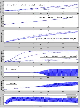
A one dimensional numerical scheme is designed with Δt = 0.0005 and N = 5 → 15.To measure the errors of the obtained results, root mean square of errors are calculated such as[17].
2 1
Root mean square of errors . . . ( ) /
NP
exact i
R M S of errors U U NP
WhereU is the obtained approximate solution while
exact
U
is the exact solution in [16]. N is the number of nodes alongx-direction while P is the number of time steps.
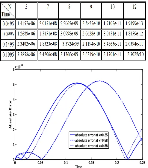
Table 1 shows that (for Δt = 0.0005 and N=10) the obtained results agree with the analytical ones [16] with
8
.
. .
10
R M S of errors
. As well as, Fig. (1-a) shows that for different times and locations, the proposed technique leadsto accurate results within absolute error
8
1.4 10
exactU
U
.Table I
Root mean square of errors for one dimensional thermal wave propagation with 1, U 1, 1, 8
o
Fig(1-a) One dimensional absolute error distribution at different instants and locations.
Fig.(1-b).Two dimensional absolute error distribution at instant 0.005990
Consider also a simple two dimensional problem with
1 2 3 4 1,
a a a a
1 2 3 4 1 2 3 4
2 b b b b f f f f 0 and g x y( , ) sin xsin y,0 x, y 1
This can be solved exactly as [19]: 2 2
( , , ) sin sin t
U x y t x ye
The design of the numerical scheme is extended to two dimensions. Table 2 shows that for Δt = 0.00001, N = 8 and M = 7, the obtained results agree with the analytical ones [19]
with 7
. . . 10
R M S of errors . Fig. (1-b) shows also (for two
dimensional problems), that the proposed technique leads to
accurate results with absolute error 6
5 10
exact
U U
Table II
Root mean square of errors for two dimensional thermal wave propagation at 0.00001, 8, 7
t N M
Fig. 2. Temperature distribution for different reaction and diffusion Parameters
Fig.2 shows that temperature increases with increasing the values of α as much as γ ˂ 8. While, it decreases with increasing the values of α as much as
8
. In general, temperature increases with increasing the values of γ. Fig. 2 shows also that the computational stability of the proposed technique is more affected with the values of α where theinstability is expected when.
2.1 .3.2.Results for Population density propagation model
In this example, it's assumed that:
1 2 0
1,
1 20
a
a
U
D
b
b
. While0 0.05 0.1 0.15 0.2 0.25
0 0.2 0.4 0.6 0.8 1 1.2 1.4x 10
-8
Time
A
b
s
o
lu
te
Er
ro
r
absolute error at x=0.25 absolute error at x=0.58 absolute error at x=0.88
0 0.1 0.2 0.3 0.4 0.5
0.6 0.7 0.8 0.9 1
0 0.1 0.2 0.3 0.4 0.5 0.6 0.7 0.8 0.9 1 0 0.5 1 1.5 2 2.5 3 3.5 4 4.5 5
x 10-6
X Y
A
b
s
o
lu
te
e
rr
o
r
1 2 2 2
1 1
( ) , ( ) ,
[1 exp( 5 t/ 6)] [1 exp( / 6 5 t/ 6)]
f t f t
2
1
( ) , 0 1.
g x x
The exact solution for such problem can be obtained as [18 ]:
2
1
U (x, t) , 0,0 1
[1 exp( / 6 x) 5 t/ 6]
exact t x
Table III shows that (for Δt = 0.0005 and N=10) the obtained results agree with the analytical ones [18] with
11
.
. .
10
R M S of errors
. As well as, Fig. 3 shows that for different times and locations, the proposed technique leads to accurate results with absolute error ≤ 10-10.Table III
Root mean square of errors for fisher equation with 1, U 1, 6 o
at
different times.
Fig. 3. Population density error fluctuations at different instants and locations
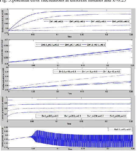
Fig. 4. Variation of the population density with the reaction and diffusion parameters.
As well as a parametric study is introduced, through fig. 4, to investigate the influence of population density by the different values of reaction and diffusion parameters. For the prescribed boundary and initial conditions, the rate of reproduction is increased with increasing both of the values for
and D. Also, the computational instability is expected when D2.1.3.3 Results for cardiac potential model
In this example, it's assumed that :
1 2 0 1, 1 2 0
a a U D b b
While:
2
1
2
1
1 1 1 (1 )
( ) (1 ) ( ) tanh ,
2 2 2 4
1 1 1 1 (1 )
( ) (1 ) ( ) tanh 2(1 )
2 2 2 4 4
1 1
( ) (1 ) (1 ) tanh 2(1 ) , 0 1, 0 1
2 2 4
f t t
f t t
x
g x x
The exact solution for such problem can be obtained as [18 ]:
Table IV shows that (for Δt = 0.0005 and N=10) the obtained
results also agree with the analytical ones [18] with
15
. . . 10
R M S of errors . As well as, Fig. 5 shows that for
different times and locations, the proposed technique leads to
accurate results within absolute error ≤ 1.2 10-14.
Table IV
Root mean square of errors for FitzHugh-Nagumo model with 0.5 at different times.
0 0.05 0.1 0.15 0.2 0.25 0
1 2 3 4 5 6x 10
-11
Time
A
b
s
o
lu
te
Er
r
o
r
0 0.05 0.1 0.15 0.2 0.25 0
0.2 0.4 0.6 0.8 1 1.2x 10
-14
Time
absolute poten
tial error
absolute potential error at x=0.25,=0.3
Fig. 5.potential error fluctuations at different instants and x=0.25
Fig. 6. Variation of the cardiac potential with the reaction diffusion and Threshold voltage parameters
Fig. 6 shows that the cardiac potential increases with
increasing the values for both of γ and . It increases also
with increasing the diffusion parameter .
While, the cardiac potential decreases with increasing the
values of . As well as the figure shows
that the computational instability is expected when .
4. CONCLUSION
A hybrid technique consists of differential quadrature method and Runge-Kutta fourth order method is employed to solve three reaction-diffusion problems. The validity of the proposed technique is proved by comparing the obtained results with the previous analytical ones. The technique
needs a small number of grid points and a little computational effort to obtain an accurate results with
absolute error 6
5 10
. Furthermore, a parametric study is introduced to investigate the influence of reaction and diffusion characteristics on behavior of the obtained results.
REFERENCES
[1] J.Opsal ,A.Rosencwaig , D.L.Willenborg ,Thermal-wave detection and Thin-film thickness measurements with laser beam deflection, Applied Optics,1983; 22(20):3169-76.
[2] R.A.Fisher ,The wave of advance of advantageous genes, Ann. Eugenics 7,1937;353–69.
[3] G. Hariharan ,K. Kannan , Haar wavelet method for solving
FitzHugh-Nagumo,International Journal of Computational and Mathematical Sciences, 2010;
4(6):560-64.
[4] Z.Y .Yan, Generalized method and its application in the higher-order nonlinear Schrodinger equation in nonlinear optical fibres, Chaos Solitons and Fractals, 2003;16(5):759-66.
[5] J.Mei ,H.Zhang , D.Jiang , New Exact Solutions For A Reaction-Diffusion Equation And A Quasi-Camassa Holm Equation, Applied Mathematics E-Notes,4 2004;85-91.
[6] E.S.Fahmy , H.A.Abdusalam , Exact Solutions for Some Reaction Diffusion Systems withNonlinear Reaction Polynomial Terms, Applied Mathematical Sciences,2009;3(11):533-40
[7] F.Zhaosheng , Traveling waves to a Reaction–diffusion equation, Discrete and continuous dynamical system, 2007;382-90. [8] L.D.Ropp ,N.J.Shadid , C.C.Ober , Studies of the accuracy of time
integration methods for reaction–diffusion equations, Journal of Computational Physics 194. 2004:544–74.
[9] R.G.Marcus , Finite-Difference Schemes for Reaction–Diffusion Equations Modeling Predator–Prey Interactions in MATLAB, Bulletin of Mathematical Biology(2007).doi: 10.1007/s11538-006-9062-3.
[10] B.Liu ,M.B.Allen , H.Kojouharov , B.Chen , et al. Finite-Element Solution of Reaction-Diffusion Equations with Advection, Computational Mechanics.1996:3-12.
[11] C.Xenophontos ,L.Oberbroeckling , On the finite element approximation of systems of reaction- diffusion equations by p/hp methods. Global Science, 2010;28(3):386-400.
[12] C. Shu , Differential quadrature and its application in engineering,
London: Springer Verlag; 2000. [13] G.Meral andM.S.Tezer , Solution of nonlinear reaction-diffusion
equation by using dual reciprocity boundary element method with finite difference or least squares method. Advances in Boundary Element Techniques, 2008;317-22.
[14] G.Meral , Solution of density dependent nonlinear reaction-diffusion equation using differential quadrature method, World Academy of Science, Engineering and Technology 41. 2010;1178-83.
[15] T.Y.Wu ,G.R. Liu , A differential quadrature as a numerical method to solve differential equations, Computational Mechanics.1999; 24(3):197–205. doi:10.1007/s004660050452.
[16] V. Kajal , Numerical solutions of some reaction-diffusion equations by differential quadrature method,Int. Appl. Math and Mech.2010; 6 (14): 68-80.
[17] W.Y.Yang ,W.Cao , T.Chung ,J. Morris , et al, Applied numerical methods using matlab, Hoboken, New Jersey: John Wiley & Sons;2005.
[18] M. Bastani ,D.K.Salkuyeh, A highly accurate method to solve Fisher’s equation, Indian Academy of Sciences. 2012;78(3):335-46. [19] E. Kreyszig , Advanced Engineering Mathematics, Columbus :