Abstract— Structured grid generation methods have been used for many years to discretize the solution domain in fluid dynamics simulations. Various differential methods have been employed for this purpose but the traditional method, which transforms a logical grid in the computational domain to a boundary-fitted grid in the physical domain, is employing a set of poison equations. In this paper a new grid generation method is introduced in which the differences between coordinates of boundary nodes of a simple initial grid and final grid are used as the boundary condition of a set of poison equations known as grid generation equations. These Poison equations are solved on the initial grid to obtain the displacement of nodal coordinates and construct the final grid. Two dimensional grid generation examples are finally presented and the grid qualities are compared with the results of an available differential grid generation method. The underlying ideas are clearly extendible to three-dimensional problems as well.
Index Term— Displacement of Boundary Nods, Initial Grid,
Structured Grid Generation, Poison Equations.
I. INTRODUCTION
Numerical solution of equations, which describe fluids flows in practical problems, is a usual approach in Computational Fluids Dynamics (CFD). This approach requires powerful discretization methods to discrete the differential terms in equations and the physical domain. Grid generation strategies are used to discrete physical domains and in the structured or unstructured generated grids [1,2], a set of elements are generated throughout the domain regarding the boundaries shapes. Accuracy and efficiency of numerical solution of equations are strongly affected by the employed grid generation methods [3,4].
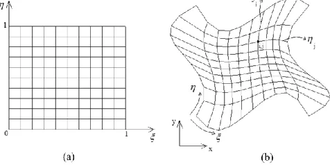
In 2D structured grid generation a physical domain is correspondent to a logical domain as shown in figure 1. The intersection of the coordinate lines
i and
j is known as the grid point
i,j in the physical domain (figure 1b) [5]. Traditional methods for mapping the unit square onto the physical domain are algebraic and differential grid generation methods. In algebraic grid generation methods the position ofAli Ashrafizadeh is with Khajeh Nasir Toosi University of Technology, Tehran, Iran. (e-mail: [email protected]).
Razieh Jalalabadi iss with Khajeh Nasir Toosi University of Technology,Tehran, Iran. (Corresponding auth, phone: +98-912-7390344;
e-mail: [email protected]).
nods in logical domain is changed to their new position in physical domain usually by using an interpolation technique [6]. But in differential grid generation methods, some constraints are used as grid generation equations and when solved, the logical grid is mapped on to the physical grid [7].
Fig. 1. The Cartesian logical grid (a) and the Physical grid (b).
A set of widely used differential grid generation equations proposed by Thompson, Thames and Mastin (TTM) [8] is:
xx
yy
P
,
(1a)
xx
yy
Q
,
(1b)
P and
Q
, the control functions which are used for better control of the distribution of grid lines, need to be known at all nodal points before the solution. Several methods have been proposed to calculate these functions some of which use some 1-dimensional or multi-dimensional interpolation techniques to calculate these functions in the domain regarding to their values on the boundaries [9,10,11]. Boundary values are calculated using (1a) and (1b) and paving layers in physical domain. Paving layers are two layers of grid generated adjacent to the boundaries using a simple algebraic method as shown in Fig. 2.In 1D interpolation techniques, the following one-dimensional formulas can be used to calculate the internal values of the source functions using their corresponding boundary values:
jC
jP
S
C
j
P
N
P
,
1
(2a)
i
C
iQ
W
C
i
Q
E
Q
,
1
(2b) In multi-dimensional interpolation techniques, the internal values of the source functions are obtained in the domain using a multi-dimensional set of formulas or through the solution of a Dirichlet boundary value problem.
Structured Grid Generation Via Constraint on
Displacement of Internal Nodes
Fig. 2. Paving layers used to calculate nodal values of P and Q near the boundaries of the physical domain.
Although some schemes have been proposed to solve (1a) and (1b) directly [11], the usual method to solve these equations is inverting equations analytically, linearizing and then solving them numerically in the logical domain. When inverted, the system of equations to be solved is:
x
P
x
Q
J
x
g
x
g
x
g
22
2
12
11
2
(3a)
y
P
y
Q
J
y
g
y
g
y
g
22
2
12
11
2
(3b) The most usual approach in the orthogonal grid generation, as another robust method in differential grid generation, is a method proposed by Ryskin and Leal [12]. Based on the assumptions of continuity and orthogonality of the coordinatelines and by imposing the orthogonality
condition,
g
12
x
x
y
y
0
, the following gridgeneration equations are obtained:
0
1
x
f
x
f
(4a)0
1
y
f
y
f
(4b)f is the distortion factor and is defined as follows:
2 2
2 2 11 22
y
x
y
x
g
g
f
(5)Calculation of the nodal values of distortion factor in the domain is a major step in the orthogonal grid generation and is discussed in a number of publications [12, 13, 14]. Most commonly, f is calculated first at the boundaries and then interpolated into the domain.
The idea underlined in the above two classical methods, is mapping logical domain onto the physical domain by two Laplace equations. These grid generation equations are in fact constraints on the mapping functions
x
(
,
),
y
(
,
)
and are solved on the logical grid.In the new structured grid generation method presented here, two linear differential equations are used to constraint the boundary displacement of an initial grid instead of mapping functions
x
(
,
),
y
(
,
)
. In the multi-dimensional interpolation technique applied, two Poison equations are solved to obtain the displacement of nodal coordinates in the physical domain.Using simple algebraic grid generation techniques, an initial grid, with the nodal coordinates
x0,y0
, can be generated for a domain as shown in Fig.3. This initial simple grid is located in the physical
x,y space. The idea is to find a way to displace the boundaries to conform them to the boundaries of target geometry in physical domain (Fig.3b). Obviously the displacement vectors which connect the initial boundary nodes to the target boundary nodes can be calculated, so a multi-dimensional interpolation technique is employed to find the displacements of the internal nodes. Here two elliptic equations are used as grid generation equations which interpolate the boundary displacements (interpolants) into the domain to generate the physical grid.Fig. 3. A simple initial grid (a) and the physical domain (b).
By using simple algebraic methods, several initial grids can be generated for any domain. The shape of initial grid can affect the computational cost and the method of solving grid generation equations.
Several possible initial grids generated for physical domains are introduced next and the discretization scheme is presented afterwards.
B. The Initial Grid
Fig. 4. Partially adapted initial grids. Adapted to the corner points(a), adapted to one boundary(b), adapted to two boundaries(c) and adapted to three
boundaries(d).
As shown in Fig. 4, the initial grid can share only the corner points with the target geometry or both the corner points and some boundaries. An FEM or FVM discretization method can be applied to solve the differential grid generation equations for all initial grids. These schemes can also be applicable for some special geometries in which a simple, not adapted initial grid may have distorted quadrilateral cells. Such a domain is shown in Fig. 5.
(a) (b)
Fig. 5. Two kinds of simple, not adapted initial grid for a special geometry
Using FEM or FVM discretization method to solve the differential grid generation equations, the user can solve the grid generation problem in multi steps. In this approach an increment of boundary displacement is used as boundary condition and an intermediate target domain is generated in each step. Each intermediate grid serves as the initial grid for the next target grid and has distorted quadrilateral cells. In the final step, the target domain is the target geometry.
Several target domains for a simple geometry is shown in Fig. 6. As it will be shown in the result section, using this technique help us to avoid folding in complex geometries and generate a smoother grid.
In this paper an Element-Based Finite Volume method has been used for the solution of grid generation equations.
(a) (b)
(c) (d)
Fig. 6. Using multi step technique in a grid generation problem
Algebraic methods can be used as a robust and fast method to generate simple or partially adapted grids. In order to generate simple initial grid, the corners of final geometry is connected with straight lines, but in partially adapted grid, the user choose some of the boundaries from final domain as adapted boundaries and generate other boundaries by connecting the corresponding corners with straight lines. After generating the boundaries of initial domain, the initial grid is generated with Transfinite Interpolation Technique (TFI) [6]. The TFI formulation used here for generating is as follows:
1 , 1 , 1 , 1 1 , 1 , , , 1 , 1 , , , 1 , 1 1 , 1 , , , , M M N M N M N N j M j M j j i i N i N i j i
R
C
R
C
R
C
R
C
R
C
R
C
R
C
R
C
R
(6)
In this formula the coordinate of node
i,j is generated by using the coordinates of boundary nodes in a (M×N) grid.C. Numerical Solution of Grid generation Equations
The equations used to interpolate the boundary displacements into the domain, in order to obtain the coordinates of internal nodal points, are two poison equations as follows:
P
,
y
x
x
x
x
2 0 2 2 0 2 2 0
(7a)
Q
,
y
y
x
y
y
2 0 2 2 0 2 2 0
(7b)The boundary conditions for these equations are the displacements calculated on the boundaries. So for partially adapted grids (as shown in Fig. 4b, c, d),
x
,
y
0
for boundaries which should be displaced to conform to the target geometry and
x
,
y
0
for adapted boundaries.Defining
)
(
),
(
x
q
y
q
x
y
(8) The integral of (7a) over the control volume with volume Vi and surface Si, is0
S
d
q
dV
q
i i S V
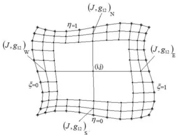
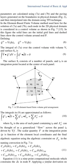
(9)The surface Si consists of a number of panels, and iP is an integration point located at the center of each panel.
Fig. 7. A 2D element-based finite volume grid arrangement.
The integrals in (9) are approximated as follows:
0
F
S
q
S
d
q
ip ip ip ip ip S ip i
(10)where Sip is the area of each panel containing iP and Fip can be thought of as a generalized „„flow‟‟ across the panel iP driven by
f
. The scalar quantity F at the integration pointip
is function of the element local coordinates and the final algebraic equation using the algebraic constraint onF
ip in the naming convection in Fig. 7 is:SE SE NE NE SW SW NW NW S S N N E E W W P P
x
C
x
C
x
C
x
C
x
C
x
C
x
C
x
C
x
C
)
(
)
(
)
(
)
(
)
(
)
(
)
(
)
(
)
(
(11)Equation (11) is a nine-point computational molecule which constrains the
x
in node P. Applying a similar derivation on (7b), another algebraic equation relating
y
i,
i and
i for each interior node is generated. These equations can be written in the following matrix forms:
A
1(
x
)
b
1 (12a)
A
2
y
b
2
(12b) The nodal values of(
x
)
i,
y
i,
i and
i prescribed for adjacent boundary nodes, are used as boundary conditions of these equations.visualize the details of performance of all methods better. Finer (2121) grids are generated in two other geometries.
The proposed grid generation equations are solved by FDM method in one step and also by FVM solver through multi steps and with two different initial grids.
In order to compare the grid quality, skewness has been chosen as a parameter to measure the quality of grids. Skewness of a cell which is between 0 and 1 measures the deviation from the orthogonality of the coordinate lines.
The computational cost in elliptic grid generation depends mostly on the cost of the solution of the grid generation equations. Both TTM equations and the proposed equations are linear poison equations and so the computational cost is similar.
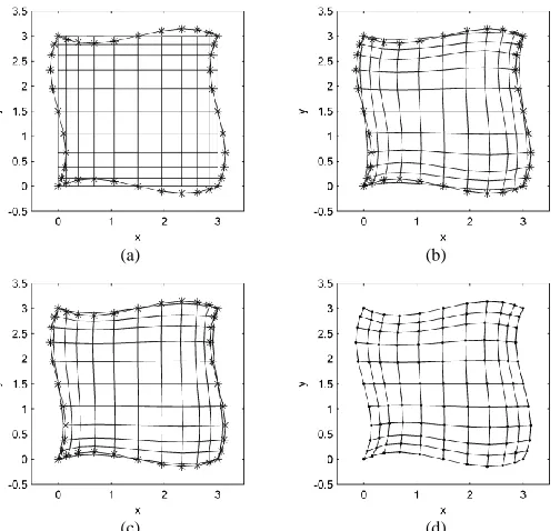
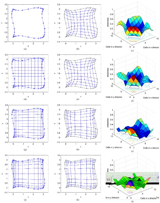
Fig. 8 shows the discretized boundaries and the (1111) grid generated by TTM and new proposed equations in first domain. The boundary nodes of physical domain are represented by * signs and initial grids for each solver is shown in Fig.8d,8g,8j. The grid generated by TTM solver and FDM solver are similar. FVM solver with simple initial grid generates a different smoother grid but as shown in Fig. 8k and 8l, by using FVM solver in multi steps with the partially adapted initial grid shown in Fig. 8j, a smoother grid is generated. As there are 10 cells along each coordinate line in the grids, each quality measure diagram shows the relevant skewness quantity for all 100 cells on a three-dimensional plot containing 1010 data points.
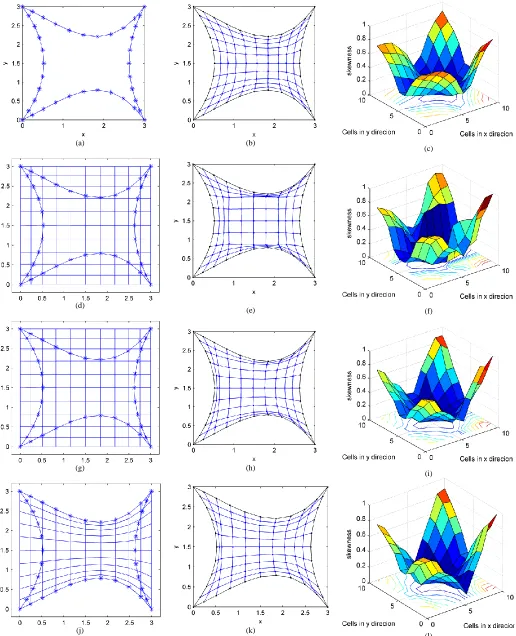
Fig. 9 shows the second domain in which TTM method generates a smooth grid but FDM implementation of proposed equations generates a folded grid. The initial grid for FDM solver and simple initial grid for FVM solver are similar for this geometry. As it is shown in Fig. 8g to 8l, the partially adapted initial grid, help FVM solver to generate a smoother grid. Again the skewness parameter is shown for all 100 cells on a three-dimensional plot.
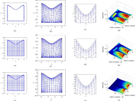
In Fig. 10 a finer (2121) grid is generated in third sample domain. FVM solver has been used only for multi step solution for this domain and initial grid for FDM and FVM solution are similar for this geometry. As shown in three-dimensional skewness plot which contains 2020 data points in the domain, FVM solver generates a smoother grid compared with FDM and TTM solver.
Fig. 11 shows the (2121) grids generated around an airfoil. The nodes around the airfoil are distributed uniformly and initial grids are shown around half of the airfoil and FVM solver has been used only for multi step solution. The skewness parameter is again shown for all 400 cells on a three-dimensional plot. As shown in Fig. 11d, h and l, TTM and
(a) (b)
(c)
(d) (e)
(f)
(g) (h)
(i)
(j) (k)
(l)
Fig. 8.The Physical domain (a), TTM grid (b),quality measures for TTM grid (c), the initial grid for FDM one step solution (d),the grid obtained by the proposed method via FDM (e), quality measures for FDM grid (f), a simple initial grid (g), the grid obtained by the proposed method via FVM for simple initial
(a) (b)
(c)
(d)
(e) (f)
(g) (h)
(i)
(j) (k)
(l)
Fig. 9.The Physical domain (a), TTM grid (b),quality measures for TTM grid (c), the initial grid for FDM one step solution (d),the grid obtained by the proposed method via FDM (e), quality measures for FDM grid (f), a simple initial grid (g), the grid obtained by the proposed method via FVM for simple initial
(a) (b) (c) (d)
(e) (f) (g) (h)
(i) (j) (k) (l)
Fig. 10.The Physical domain (a), TTM grid (b), a larger view of a section of north boundary (c), quality measures for TTM grid (d), the initial grid for FDM one step solution(e),the grid obtained by the proposed method via FDM (f), a larger view of a section of north boundary (g), quality measures for FDM grid (h), a
(a) (b) (c) (d)
(e) (f) (g) (h)
(i) (j)
(k) (l)
Fig.11.The Physical domain (a), TTM grid (b), a larger view the grid around airfoil (c), quality measures for TTM grid (d), the initial grid for FDM one step solution(e),the grid obtained by the proposed method via FDM (f), a larger view the grid around airfoil (g), quality measures for FDM grid (h), a partially adapted initial grid (i), the grid obtained by the proposed method via FVM for partially adapted initial grid(j), a larger view the grid around airfoil (k), quality measures for FVM solution of equations on partially adapted initial grid (l).
IV. CONCLUSION
In this paper, after reviewing the two most commonly used classical methods of elliptic grid generation, a new elliptic grid generation method was proposed. In this method the general idea was similar to the previous methods; solving a multi-dimensional interpolation problem, but the interpolants were different parameters. In the simple differential method presented, an initial grid was deformed to conform to the given physical boundaries and the differences between coordinates of boundary nodes of an initial grid and the final grid are used as interpolants. Two poison equations are introduced as grid generation equations and the boundary conditions are the interpolants discussed. FDM scheme in one step and FVM scheme in both one step and multi steps have been used to solve the equations and the skewness diagram is presented to study the smoothness of final grids better. FVM solver generates smoother grids with better quality especially in complex geometries and with a partially adapted grid as an initial grid. As a result, it can be mentioned that the proposed
method solve grid generation problem from a different viewpoint and in general this method is computationally similar to TTM method while both methods provide grids with comparable qualities.
REFERENCES
[1] R. W. Noack, D. A. Anderson, “Solution-Adaptive Grid Generation using Parabolic Partial Differential Equations”,
Journal of The American Institute of Aeronautics and
Astronautics, Vol. 28, pp.1016-1023, 1990.
[2] D. L. Marcum, N. P. Weatherill, “Unstructured Grid Generation Using Iterative Point Insertion and Local Reconnection”, Journal
of The American Institute of Aeronautics and Astronautics, Vol.
33, pp. 1619-1625, 1995.
[3] C. Conti, R. Morandi, R. M. Spitaleri, “An algebraic–elliptic algorithm for boundary orthogonal grid generation”, Journal of
Applied Mathematics and Computation, Issue 162, pp. 15–27,
2005.
[4] Y. Zhang, Y. Jia, S. S.Y. Wang, “2D nearly orthogonal mesh generation with controls on distortion function”, Journal of
Computational Physics, Issue 218, pp. 549–571, 2006.
Conference, Ecole Polytechnique, Montreal, Canada, May 25-28, 2009.
[6] Peter R. Eiseman, Yung K. Choo and Robert E. Smith, “Algebraic Grid Generation with Control Points”, Finite elements fluid, Vol. 8, pp. 97-116, 1992.
[7] P. Barrera-Sánchez, F.J. Domínguez-Mota, G.F. González-Flores, Longina J.Castellanos Noda y Ángel A.Pérez Domínguez, “Area Functionals For High Quality Grid Generation”, 4º Congreso Internacional, 2º Congreso Nacional sobre Métodos Numéricos en Ingeniería y Ciencias Aplicadas, México, 2007.
[8] J. F. Thompson, F. C. Thames and C. W. Mastin, “Automatic Numerical Generation of Body-Fitted Curvilinear Coordinate System for Fields Containing Any Number of Arbitrary Two-Dimentional Bodies”, Journal of Computational Physics, Vol. 15, pp. 299-319, 1974.
[9] P.D.Thomas and J.F.Middlecoff, “Direct Control of the Grid Points Distribution in Meshes Generated by Elliptic Equations”,
Journal of the American Institute of Aeronautics and
Astronautics, Vol. 18, pp. 652-656, 1980.
[10] A. Ashrafizadeh, G. D. Raithby, “Direct Design Solution of the Elliptic Grid Generation Equations”, Journal of Numerical Heat
Transfer, Vol. 50, pp. 217-230, 2006.
[11] S. P. Spekreijse, “Elliptic Grid Generation Based on Laplace Equations and Algebraic Transformations”, Journal of
Computational Physics, Vol. 118, pp. 38–61, 1995.
[12] G.Ryskin & L.G.Leal, “orthogonal mapping”, Journal of
Computational Physics, Vol. 50, pp. 71–100, 1983.
[13] Andrei Bourchetin and Ludmila Bourchetin, “On generation of Orthogonal Grids”, Journal of Applied Mathematics and
Computing, Vol. 173, pp. 767-781, 2006.
[14] R. duraiswami and A. Prosperetti, “Orthogonal Mapping in Two Dimensions”, Journal of Computational Physics, Vol. 98, pp. 254-268, 1992.