Techniques for Optimization in Time Delay Estimation from Cross Correlation Function

Techniques for Optimization in Time Delay

Estimation from Cross Correlation Function

1.

Noor Shafiza Mohd Tamim,

Farid Ghani

1.

School of Computer and Communication Engineering, 2. School of Computer and Communication Engineering

1.

Universiti Malaysia Perlis, 2. Universiti Malaysia Perlis [email protected]

2._{[email protected]}

Abstract-- Measuring delay using cross correlation technique with signals that are corrupted by noise and are received at two spatially separated sensors often result incorrect measurement. This paper presents a new technique that is Hilbert transform of FFT pruned cross correlation function to improve the accuracy of time delay estimates. To investigate the performance of this technique, frequency algorithms are provided to generate synthetic complex base band signals. For each iteration, it generates two sets of signal. We have to specify input parameters to the simulation model any time delay of signal 2 from signal 1, length and number of complex base band signals to be generated. S uch model imitate real -life system, and by varying the uncorrelated complex base band signals to various S NR conditions, further analysis can be performed to compare the performance of this new technique with other existing techniques such as parabolic interpolation, zero crossing of Hilbert transform and FFT pruning.

Index Term-- FFT Pruning, Hilbert Transform, cross correlation, analytic signal, quadrature demodulation

I. INTRODUCTION

Cross correlation method(CCM) is a well known technique for measuring time delay estimation(TDE) and is being used in various communication and voice processing systems[1].This paper examines problems associated with time delay estimation using conventional cross correlation method when two signals corrupted with noise(assuming noise is white) are received at two spatially seperated sensors and when both signals are not integral multiple of the sampling period due to low sampling frequency [5]. Under these circumstances, received signals will not overlap exactly during correlation process causing inaccuracy in the delay estimates. However, by interpolating the correlation function of two received complex base band signals, new peak that represents the new time delay estimate will be compared with the peak from non-interpolated cross correlation function. Therefore, we can prove if the results after interpolation are better when actual delay value is known. In this study, a new technique to improve time delay estimates is proposed. This technique is based on Hilbert transform of FFT pruned cross correlation function. Its performance is compared with the existing technique like FFT pruning, parabolic interpolation and zero crossing of Hilbert transform. For generation of synthetic complex base band signals, all the stages of the algorithm are implemented in frequency domain.

The initial synthetic signal is generated with infinite SNR prior to varying this synthetic signals to other various SNR conditions.

II. COM PLEX BASEBAND SIGNALS GENERATION A. Complex Base Band Signal With Infinite SNR

In this simulation model, the length of the signal to be generated within finite time observation is given by: L2k k=0,1,2,….P (1) This signal length is chosen so that we can later use FFT pruning method. Delay to the first L-point discrete time random signal x1[n] that indicates the time of signal

propagation from the transmitter to receiver 1 is defined as a fix delay value, d1=(L/4)∆T with ∆T is normalized time

interval. Delay of signal received at receiver 2, d2 that will

be input by user during the simulation must be greater than d1 and the maximum delay value allowed between x2[n] and

x1[n] is d2<(L/4)∆T. x2[n] can be computed directly as in (6)

when d2 is integer. However, (6) cannot be used when d2 is

non integer, since only the value of the discrete time signal at integer location is known. Therefore, unsampled points of x2[n] when d2 is non integercan be computed using inverse

CTFT of the DTFT x2[n].

 



 



d e

X d

n x n

x_{2 1 2 1( )} j (n d2)

2 1 ] [ ]

[ 





 (2)

) (

)) ( sin( 2

1 ] [

2 2 )

(

2 2

d n

d n d

e n

h j n d

  





 

   



 

(3)

[ ] ₁[ ] ₂[ ] 1

2n x k h n k

x N

o k

 









, d2≠integer (4)

Next stage is to transform x1[n] and x2[n] into its

frequency domain simply by taking its FFT. If d2 is an

integer, x2[n] can be transformed directly in its frequency

domain as in (5) by using delay property in DFT:







 1 2 /

1

1[ ] [ ]

L

o n

L kn j

e n x k

X  (5)

X_2[k_]X_1[k_].ej2kd2/N _{, d}

2=integer (6)

Next stage filters the L-points complex signals with a band pass filter and yields XBP[k]. A simple band pass filter is a

combination of zeros padding which pin down the low frequency components prior followed by any type of window function such as Tchebyshev window to pin up the high frequency components. Since the L-point signal spectrum is evaluated from 0Hz to twice the maximum frequency, 2fmax of the signal, therefore the first half of L

can be applied simply by deleting the negative frequency half of the filtered signal [4]. Discrete time analytic band pass signal is defined in frequency domain as :

   

   

 

    

 





1 1

0 ] [

] [ 2

0 ]

[

] [

L k 2 L for

2 L k for k X

1 -2 L k 1 for k X

k for k X

k X

BP BP BP

BP

The new centre frequency of analytic band pass signal will be down converted to base band centered around 0Hz by performing quadrature demodulation [6].

B. Complex Base Band Signal with Various SNR Conditions

Generating complex base band signals with various SNR conditions can be done simply by adding scaled random noise to signal with infinite SNR. The SNR values for each case can then be computed as following:

    

 

    

 









 



| ] [ |

| ] [ |

log 20 )

( ₁

0 1

0

10 _L

n a L

n CB

n r

n x

dB

SNR (8)

where xCB[n] is complex base band signal with infinite SNR

and ra[n] is the scaled random noise with a as the noise

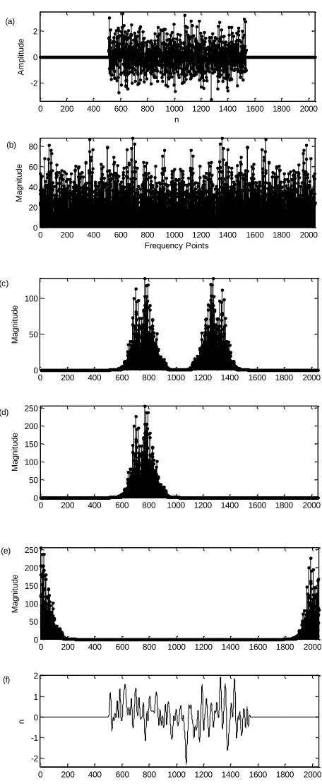
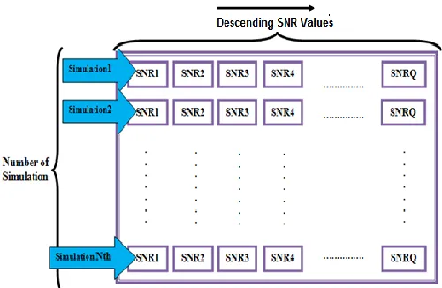
coefficient ranging from 0.1 to 2.0 with increment step size of 0.1. However, SNR range in this simulation model is not restricted within this range, but it can be further decreased by increasing noise coefficient value. Fig. 2 depicts averaging from 50 simulations of generating complex base band signals to standardize decrement in SNR values as the noise coefficient value is increased. The final outcome of the whole simulation model is as shown in Fig. 3 which generates received complex base band signals x1[n] and

x2[n] for various SNR conditions ranging from 16dB down

to -11dB. These sets of data are ready for correlation process prior to applying interpolation to the cross correlation function for optimizing the time delay estimation.

0 200 400 600 800 1000 1200 1400 1600 1800 2000 -2

0 2

n

A

m

p

lit

u

d

e

0 200 400 600 800 1000 1200 1400 1600 1800 2000 0

20 40 60 80

Frequency Points

M

a

g

n

it

u

d

e

(a)

(b)

0 200 400 600 800 1000 1200 1400 1600 1800 2000 0

50 100

M

a

g

n

it

u

d

e

0 200 400 600 800 1000 1200 1400 1600 1800 2000 0

50 100 150 200 250

M

a

g

n

it

u

d

e

(c)

(d)

0 200 400 600 800 1000 1200 1400 1600 1800 2000 0

50 100 150 200 250

M

a

g

n

it

u

d

e

0 200 400 600 800 1000 1200 1400 1600 1800 2000 -2

-1 0 1 2

n

(e)

(f)

Fig. 1. (a) Delayed random signal. (b) Signal in transform domain. (c) Signal after band pass filtering. (d) Analytic Band pass signal. (e) Signal after quadrature demodulation. (f) Complex base band signal infinite SNR

Fig. 2. SNR values versus Noise Coefficients, a

Fig. 3. Automated Synthetic Complex Baseband Signals Generation

III. TIM E DELAY ESTIM ATION

A. Time Delay Estimation from CCM

By having N x Q sets of received complex base band signals x1[n] and x2[n], we can directly correlate these two signals to

obtain the time delay estimate.

N

N n

CB CB

CB [] [ ] 2[ ]

1

) 1 (

1 2

,

1 





  

From each correlation function, information on amplitude and its corresponding delay index for maximum peak and its two left and right neighboring points will be extracted. This information is required for parabolic interpolation. Moreover, information on the maximum peak can be used to perform analysis on the accuracy of time delay estimate that is obtained from the conventional cross correlation meth od. The mean square error of delay estimate is given as:



B. FFT Pruning to CCM

Besides taking time delay estimates directly from cross correlation method, we apply FFT pruning to the cross correlation function to see if the accuracy of the delay estimates value can be improved. Conventional FFT pruning based on integral of power of two has been widely used and independently discovered by many and it is proved to be satisfactory if the data was band limited or nearly so [7]. FFT pruning is also known as FFT interpolation. It is an algorithm which eliminates operations on zeros, when number of input points is less than number of transform points, the number of butterflies may be reduced [3]. This is

done by appending zeros between the new and old Nyquist frequency when it is in transform domain and this is equivalent to increasing the sampling frequency in order to obtain high resolution of signal in its time domain after taking its inverse Fourier transform. Consider if we have a set of data, x[n∆T] of length N where the normalized sampling interval ∆T is 1 and n=0,…,N-1. We wish to interpolate to any factor of interpolation, Ti-1 as long N and

Ti-1 is an integral of power of 2.

NT MT_i (11) Therefore, length of sequence after FFT pruning is given by

M:

N T

T M

i



 (12)

Number of zeros to be inserted between the old and new Nyquist frequency is simply M-N. Length of correlation function of two N length sequences is given by 2N-1. Therefore, prior to employing FFT pruning to the cross correlation function, we must do single zero padding at the end of the correlation sequence to yield sequence length that is integral of the power of two. The following algorithm shows FFT pruning approach being applied to the cross correlation function in its transform domain, X[k] for peak detection using any factor of interpolation, Ti-1.

        

        

   

  

  

   

  

1 1

2 ], [

2 0

1 2 0 1

], [ ] [

M m 2 N M for N k 2 N k X

2 N -1) -(M m 2 N for

N m for 2 N k 0 k X

m

X (13)

We take the inverse Fourier transform of X[m] to get the interpolated cross correlation function. In simulation, lag indices, k is from –(N-1) to N-1 with normalized time interval ∆T equals to one, and after FFT interpolation, lag indices k can be defined as:

1 1

1 ,...,( 1)

2 ) 1 ( , 1 ) 1

(   _    _    _

 

i i

i T

j N

T N T N

k (14)

C. Parabolic Fit Interpolation

Parabolic interpolation is one of the most widely used techniques to locate the optimum peak of the correlation function. Generally, the magnitude of the correlation function has a shape close to the Gaussian function, and therefore parabolic interpolation can be considered as an appropriate technique to get good time delay estimation. In this application, parabolic fitting is performed in the vicinity of maximum discrete point correlation coefficients . A parabola uses a second order polynomial:

yax2bxc (16) It can be described uniquely by the peak from cross correlation function and its two left and right neighboring points, so that the maximum point of the parabolic curve passes through all the three points:

y[x_1]ax_2₁bx_1c (17a) y[x₀]ax₀2bx₀c (17b)

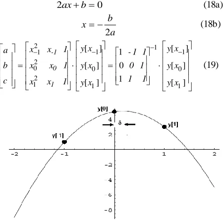
Since we have three input sample values and their corresponding indices, the x- value returned is the deviation of the parabola peak from the second (center) point indicated as δ in Fig. 4. It is straight forward that the derivative at the maximum peak, dy/dx of (12) which represents the slope is zero. Therefore:

2axb0 (18a) a b x 2 

 (18b)

                                                                  ] [ ] [ ] [ 1 0 1 ] [ ] [ ] [ 1 0 1 1 1 0 1 2 1 2 0 2 1 x y x y x y 1 1 1 0 1 1 x y x y x y 1 x x 1 x x 1 x x c b a 1 0 1 (19)

Fig. 4. Parabolic Fit Interpolation

D. Zero Crossing of Hilbert Transformation

The zero crossing of Hilbert transformed correlation function can also be employed to improve time delay estimation. We can visualize information of delay estimates in a more convenient way as the derivative to the cross correlation function converts the maximum of cross correlation to zero crossing [12]. Hilbert transform to the cross correlation function, y(t) in time and frequency domain is defined by (20) and (21) respectively.

 

 t d

t y t y



 1 ()

) ( ^

(20)

( ) ( ) ( /2)sgn( ) ( )( sgn( )) ^

 



 Y e   Y j

Y  j   (21a)

          0 for 0 for 0 for     1 0 1 )

sgn( (21b)

From (21), clearly can be seen that Hilbert Transform has the effect of shifting the negative frequency components of y(t) by +900 and the positive frequency components by -900. In frequency domain, correlation function can be represented as the multiplication process and Hilbert transform to the correlation function is simply implemented by multiplying the Hilbert transform transfer function H(ω)=-jsgn(ω) to the correlation function y[n].

        1 -L n 0 for 1 -2L n L for n x n x 0 ] [ ]

[ 1,2

2 ,

1

  

 H X X

Y   

Apart from that, Hilbert transform to the correlation function can be obtained by taking its analytic signal to the correlation function where the real part of analytic signal is the real value of the correlation function and the imaginary

part is the Hilbert transformed of the correlation function [4].

-250 -200 -150 -100 -50 0 50 100 150 200 250 -40 -20 0 20 40 60 A m p lit id e

-250 -200 -150 -100 -50 0 50 100 150 200 250 -50 0 50 lag index A m p lit u d e

Fig. 5. (a) Correlation function. (b) Hilbert T ransformed Correlation Function

From Fig. 5(a), when the correlation function passes through a maximum, its Hilbert transform will pass through zero [12]. In real measurement, it often occurs that the received signal does not hit the multiple of sampling instant during a sampling process by ADC. As a result, the zero crossing may occur at a point not explicitly defined by the data points. Therefore a simple linear interpolation between two data points which are the local minimum and maximum lie below and above zero respectively can be employed in order to locate the actual location for the delay estimates . Another advantage of using this technique is when peak is fairly broad, we do not have to the take the derivative of the cros s correlation function to locate the maximum [12]. This enables a very simple search process to be used to determine the delay.

E. Hilbert Transform of FFT Pruned Correlation Function

Hilbert transform of FFT pruned cross correlation function is a new technique proposed. It is a combination of two techniques, which are FFT pruning and Hilbert transform. FFT pruning helps to increase the resolution of time intervals, ∆T and by taking Hilbert transform to the FFT pruned cross correlation function, it is more convenient for us to focus on smaller area prior to employ linear interpolation between the two maximum and minimum data points lie below and above zero respectively.

-70 -60 -50 -40 -30 -20 -10 0 10 20 30 40 -20

0 20

-70 -60 -50 -40 -30 -20 -10 0 10 20 30 40 -20

0 20

-70 -60 -50 -40 -30 -20 -10 0 10 20 30 40 -20

0 20

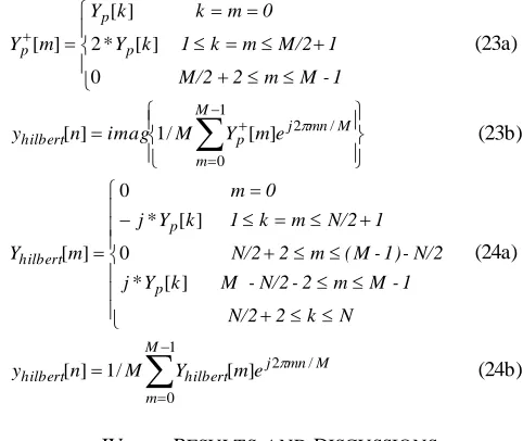
A further advantage of using this technique compared to FFT pruning technique only is FFT pruning technique provides time interval resolution limited to 2k while linear interpolation may be performed for any factor not limited to 2k. The following algorithm shows Hilbert transform of FFT pruned cross correlation function Yp[k] of length M, and

there are two methods. The first method is by taking analytic signal to the FFT pruned Yp[k]. In the second

method is by applying +900 phase shift to the FFT pruned Yp[k]:

    

  

   

  



1 -M m 2 M/2

1 M/2 m k 1 k Y

0 m k k Y

m

Y p

p

p

0 ] [ * 2

] [

]

[ (23a)

   

   







  1

0

/ 2 ] [ /

1 ]

[

M

m

M mn j p

hilbertn imag M Y me

y  (23b)

  

   

 

  

 

  

    





N k 2 N/2

1 -M m 2 -N/2 M k Y j

N/2 -1) -( M m 2 N/2

1 N/2 m k 1 k Y j

0 m

m Y

p p

hilbert

] [ * 0

] [ * 0

]

[ (24a)



 

1

0

/ 2 ] [ /

1 ] [

M

m

M mn j hilbert

hilbertn M Y me

y  (24b)

IV. RESULTS AND DISCUSSIONS

Generation of complex base band signals x1[n] and x2[n] is

very useful in investigating the performance of interpolation techniques that have been applied to the cross correlation function in order to optimize time delay estimates. Fig. 7 compares the result of the accuracy in estimating time delay with and without employing interpolation . Number of iteration is 100, delay of signal x2[n] from signal x1[n] is set

11.3∆T and the factor of interpolation in FFT technique is 8 which yields sampling interval resolution of 0.125∆T. It can be seen that interpolated time delay estimates are improved for all decreasing SNR conditions. Regardless with or without interpolation, the error is increasing as SNR value is decreasing.

Fig. 7. T ime Delay Estimates with Various SNR Conditions

Parabolic interpolation which is the simplest technique to be implemented is seen to be a good technique by looking at overall SNR conditions. Zero crossing of Hilbert transform provides poor result at low SNR conditions. At high SNR conditions above 11dB, FFT pruning provides accurate time delay estimates for the case that often occur when both signals to be correlated do not overlap exactly due t o low sampling frequency by ADC. For example, if delay of signal 2 from signal 1 is 100.125∆T, (we assume transmitter and receivers are located at the same horizontal axis), peak after interpolation with factor interpolation of 8 is exactly at lag index 100.125∆T. Definitely in real scenario decimation value of both signals is not restricted to multiple of the sampling interval resolution, but may fall at any value. For example at 100.121∆T, the accuracy of delay estimates can be further optimized by taking Hilbert transformation to the FFT pruned cross correlation function. Table I concentrates on time delay estimation after all the four interpolation techniques have been applied to the cross correlation function. Both signals are considered here with high SNR value ranging from 5dB to 21dB. Delay of signal 2 from signal 1 has been set as 100.121∆T. It can be seen that zero crossing of Hilbert transform technique and Hilbert transform of FFT pruned cross correlation function technique provide good results, but with a slightly higher computational load.

TABLE I

INTERP OLATED TIME DELAY ESTIMATES AT HIGH SNRCONDITIONS

a SNR

(dB)

Parabolic FFT Pruning Hilbert Transform _{FFT Pruned of Hilbert Transformed}

Time Delay

(∆T)

Error |∆T|

Time Delay (∆T)

Error |∆T|

Time Delay

(∆T)

Error |∆T|

Time Delay

(∆T) Error _|∆T|

0.050 21 100.1249 0.0001 100.125 0.004 100.125 0 100.125 0 0.070 19 100.0910 0.03422 100.125 0.004 100.125 0 100.125 0 0.090 17 100.0747 0.05031 100.125 0.004 100.125 0 100.125 0 0.105 15 100.0329 0.09211 100.125 0.004 100.125 0 100.125 0 0.130 13 100.0019 0.1231 100.125 0.004 100.125 0 100.125 0 0.165 11 99.9686 0.1564 100.125 0.004 100.125 0 100.125 0

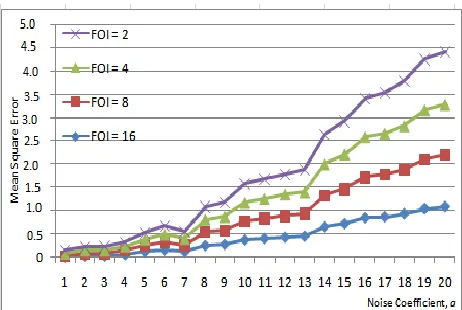
Fig. 8 compares performance of FFT interpolation technique applied to the cross correlation function for various factor of interpolation. It begins with factor of interpolation 2 and yields time interval resolution of 0.5∆T up to factor of interpolation 8 and yields time interval resolution as small as 0.0625∆T. It can be seen that the accuracy of time delay

Fig. 8. T ime Delay Estimates for Various Factor of Interpolations

VII. CONCLUSIONS

Interpolation techniques applied to the cross correlation function have proved to produce better time delay estimates. Parabolic method is easy to implement as it only uses the peak and its two neighboring values . FFT technique requires all correlation function samples, and is complex in computation process. However, at high SNR condition when both signals to be correlated do not overlap exactly , parabolic technique can never produce zero error as compared to the other three interpolation techniques. Zero crossing of Hilbert transform provides good results at high SNR conditions. Hilbert transform of FFT pruned correlation function technique provides perfect time delay estimates when both signals to be correlated have delay that is not multiple of sampling instant. The accuracy of all the techniques decreases as SNR value increases . Cross correlation method is the most basic time domain approach often used to resolve the time delay estimation problem in various applications, for example in radar and sonar technologies. The received signal reflected from the target is the delayed version of the transmitted signal and by measuring the delay, we can estimate the location of the target [11]. However, often the detection problem gets more complicated in practice as the received signal is corrupted with additive random noise from the transmission medium or electrical monitoring system as well.

REFERENCES

[1] Jacob Benesty, Jingdong Chen, Yiteng Huang, ‘T ime Delay Estimation via Linear Int erpolation and Cross Correlation’, IEEE Transactions on Speech and Audio Processing, Volume-12, No-5, September 2004

[2] Jingdong Chen, Yiteng (Arden) Huang, Jacob Benesty, ‘T ime Delay Estimation via Multichannel Cross Correlation’, IEEE International Conference on Audio, Speech and Signal Processing ICASSP 05, Volume-3,page iii/49-iii52, May 2005

[3] Sverre Holm, ‘FFT Pruning Applied to Time Domain Interpolation and Peak Localization’, IEEE Transactions on Acoustics, Speech, and Signal Processing, Volume-35, No-12, December 1987

[4] S. Lawrence Marple, ‘Computing the Discrete Time Analytic Signal via FFT ’, IEEE Transactions on Signal Processing, Volume-47, No-9, September 1999

[5] Xiaoming Lai, Hans Torp, ‘Interpolation Methods for T ime Delay Estimation Using Cross Correlation Method for Blood Velocity Measurement’, IEEE Transactions on Ultrasonics, Ferroelectrics, and Frequency Control, Volume-46, No-2, March 1999 [6] S. Lawrence Marple, ‘Estimating Group Delay and Phase Delay via

Discrete T ime Analytic Cross Correlation’, IEEE Transactions on Signal Processing, Volume-47, No-9, September 1999

[7] William G. Hawkins, ‘FFT Interpolation for Arbitrary Factors: A Comparison to Cubic Spline Interpolation and Linear Interpolation’,

IEEE Nuclear Science Symposium and Medical Imaging Conference, Vol. 3, On page(s): 1433-1437 vol.3, 1994

[8] E. Oran Brigham, ‘The Fast Fourier Transform: An Introduction to Its T heory and Application’, Prentice Hall, November 1973 [9] Win C. van Etten, ‘Introduction to Random Signals and Noise’,

Wiley, 2005

[10] Patrick Gaydecki, ‘Foundations of Digital Signal Processing: Theory, Algorithms and Hardware Design’, T he Institution of Electrical Engineers, 2004

[11] Sanjit K. Mitra, Digital Signal Processing: A Computer Based Approach, McGraw Hill, 2006