e-ISSN: 2278-067X, p-ISSN: 2278-800X, www.ijerd.com
Volume 12, Issue
2
(
Febr
uary 2016), PP.26-40
Simulation of Two-Phase Flow and Heat Transfer in
Shell-Tubes Heat Exchanger
Ahmed A. Maraie
1, Ali Ahmed M. Hassan
2, Mohamed Salah Hassan
2,
TahaEbrahim M. Farrag
3, Mamdouh M. Nassar
11Department of Chemical Engineering, Faculty of Engineering, Minia University, Minia, Egypt
2Mechanical Power Engineering & Energy Department, Faculty of Engineering, Minia University, Minia, Egypt 3
Department of Chemical Engineering, Faculty of Engineering, Port Said University, Port Said, Egypt
Abstract:-Heat transfer of two-phase flow in shell and tubes heat exchanger (HEx.) were investigated
experimentally and simulated using a computational fluid dynamics (CFD) for a two-phase flow. Heat transfer to flow of mixture (air–water) through tubes side heating by a flow of hot water in shell side was considered in this study. A computer model using flow simulation of SolidWorks® Premium 2014 edition has been developed and performed for a studied heat exchanger by applying several operating conditions. Important flow quantities of mixture of (air-water) such as void fraction, liquid velocity, pressure drop and temperature distribution were estimated at different inlet flow rates.Comparison of the obtained results of temperature, pressure drop and overall heat transfer coefficients show good agreement with experimental data. The results contour plots reveal that an appearance of the gas phase into the liquid stream play an important role in the distribution of phase, velocity, pressure, and temperature in tubes of the shell-tubes HEx. Results generally indicate to that the increasing of overall heat transfer coefficient, and pressures drop as ReSG increases for a fixed low ReSL due to
increase of turbulence and mixing action in the water stream as result of a continuous interaction of the two-phase in tubes of HEx. Thus, the performance of shell and tubes heat exchanger is more efficient and improved for two-phase more than one phase flow in tubes. So, the simulation model by a CFD has more ability to capture and the interpretation for main flow features compared to an experimental model.
Keywords:-Simulation; Shell and Tubes; SolidWorks; CFD; Air–water; Two Phase.
I.
INTRODUCTION
Heat exchanger is a mechanical device which is used for the purpose of exchange of heat between two fluids at different temperatures. There are various types of heat exchangers available in the industry, however the shell and tubes type heat exchanger is probably the most used and widespread type of the heat exchanger’s classification. It is used most widely in various fields such as oil refineries, thermal power plants, chemical industries and many more. This high degree of acceptance is due to the comparatively large ratio of heat transfer area to volume and weight, easy cleaning methods, easily replaceable parts etc. Shell and tubes type of heat exchanger consists of a number of tubes through which one fluid flows. Other fluid flows through the shell which encloses the tubes. The heat exchange between the two fluids takes through the wall of the tubes [1].
In the literature the design and analysis of shell and tubes type of heat exchanger has been done through various modes viz. theoretically, experimentally, by making software models, etc. Due to a limitation of experimental data setup, computer simulations are alternatively used to help understand the flow behavior. So the intense development for CAD and CAE facilities have given a good tools to the actual working conditions, and henceforth find their accuracy and compatibility with the desired functions. Computational fluid dynamics is a powerful tool for fluid dynamics and thermal design in industrial applications, as well as in academic research activities. Based on the current capabilities of the main CFD packages (such as FLOTHERM, ICEPAK, FLUENT, Ansys, SolidWorks, and CFX) suitable for industry and the nature of industrial applications, understanding the physics of the processes, introducing adequate simplifications and establishing an appropriate model are essential factors for obtaining reasonable results and correct thermal design [2, 3].
efficiency and economical design or optimization. Although the most existent designs use experimental methods, but as an outcome of growth and development of numerical methods and the soft-wares which can solve the PDEs, the tendency for analyses of fluid flow and heat transfer are appeared. So because of expense and time wasting of empirical assessments and hardness of turbulence conditions verification and details in heat exchangers, a reliable modeling is desired for a two-phase flow of a shell and tubes heat exchanger designing.
II.
THEORETICAL ANALYSIS
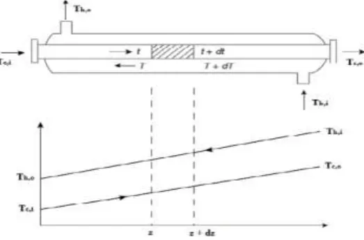
The main assumptions applied for the energy balance on the tested heat exchanger shown in Fig.(1) are;
Mass flow rate is constant.
There is no heat loses to environment.
No shaft work is done by the fluid.
Fig. 1: Heat Transfer in Counter-Current Heat Exchanger
Kays and London [10] came up with a method in 1955 called the effectiveness–NTU method, which greatly simplified heat exchanger analysis. This method is based on a dimensionless parameter called the heat transfer effectiveness ε, defined as [11];
𝜀 =
𝑄Q𝑚𝑎𝑥
=
𝐴𝑐𝑡𝑢𝑎𝑙 𝑒𝑎𝑡 𝑡𝑟𝑎𝑛𝑠𝑓𝑒𝑟 𝑟𝑎𝑡𝑒
𝑀𝑎𝑥𝑖𝑚𝑢𝑚 𝑝𝑜𝑠𝑠𝑖𝑏𝑙 𝑒 𝑒𝑎𝑡 𝑡𝑟𝑎𝑛𝑠𝑓𝑒𝑟 𝑟𝑎𝑡𝑒………….. (1)
The actual heat transfer rate in a heat exchanger can be determined from an energy balance on the hot or cold fluids and can be expressed as;
𝑄 = 𝐶
𝑐𝑇
𝑐,𝑜𝑢𝑡− 𝑇
𝑐,𝑖𝑛= 𝐶
𝑇
,𝑖𝑛− 𝑇
,𝑜𝑢𝑡 ………….. (2)where
𝐶
𝑐= 𝑚
𝑐𝐶𝑝
𝑐 and𝐶
= 𝑚
𝐶𝑝
are the heat capacity rates of the cold and the hot fluids, respectively. Also, to determine the maximum possible heat transfer rate in a heat exchanger, must be recognize that the maximum temperature difference in a heat exchanger is the difference between the inlet temperatures of the hot and cold fluids. That is;∆𝑇 = 𝑇
,𝑖𝑛− 𝑇
𝑐,𝑖𝑛………….. (3)Therefore, the maximum possible heat transfer rate in a heat exchanger is;
𝑄
𝑚𝑎𝑥= 𝐶
𝑚𝑖𝑛𝑇
,𝑖𝑛− 𝑇
𝑐,𝑖𝑛 ………….. (4)where
𝐶
𝑚𝑖𝑛 is the smaller of𝐶
and𝐶
𝑐.𝑄 = 𝜀𝑄
𝑚𝑎𝑥= 𝜀𝐶
𝑚𝑖𝑛𝑇
,𝑖𝑛− 𝑇
𝑐,𝑖𝑛 ………….. (5)The effectiveness of a heat exchanger depends on the geometry of the heat exchanger as well as the flow arrangement [11-13]. Also, the effectiveness relations of the heat exchangers typically involve the dimensionless group is called the number of transfer units (NTU) and is expressed as [11];
𝑁𝑇𝑈 =
𝑈𝐴𝐶𝑚𝑖𝑛
………….. (6)
In heat exchanger analysis, it is also convenient to define another dimensionless quantity called the capacity ratio
𝑐
as [11];𝑐 =
𝐶𝑚𝑖𝑛𝐶𝑚𝑎𝑥 ………….. (7)
The effectiveness of a heat exchanger is a function of the number of transfer units NTU and the capacity ratio
𝑐
. That is [11];𝜀 = 𝑓(𝑁𝑇𝑈, 𝑐)
………….. (8)Effectiveness relations have been developed for a large number of heat exchangers as shown in many textbooks [11-13]. The value of the effectiveness ranges from 0 to 1. The effectiveness of a heat exchanger is independent of the capacity ratio
𝑐
for NTU values of less than about 0.3 [11]. NTU relation with known𝑐
and𝜀
for an one-shell and one-tubes pass heat exchanger with a counter current flow is [11];𝑁𝑇𝑈 =
1𝑐−1
𝑙𝑛
(
𝜀−1
𝜀𝑐 −1
)
………….. (9)Then with known a specification dimensions of a heat exchanger, the overall heat transfer coefficient can be calculated using Eqn. (6) after rearrangement as follow;
𝑈 =
𝐶𝑚𝑖𝑛 𝑁𝑇𝑈𝐴 ………….. (10)
So, using Eqn. (10) to evaluate overall heat transfer coefficient (U) then plot as a function of Reynolds number of cold water (ReSL) and air (ReSG) at superficial average velocities.
III.
EXPERIMENTAL FACILITY AND MEASUREMENTS TECHNIQUE
A. Experimental Setup
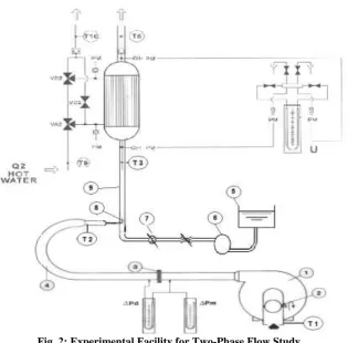
A schematic diagram of the experimental facility is presented in Fig.(2). The water was drawn from a water tank (5) by a centrifugal pump (6). The water flow-rate was controlled by a flow regulator and measured by a calibrated Rotameter (7) with an accuracy of ±2%. The air was delivered by a centrifugal blower (1) through a steel pipe connect with reduction pipe (4) then ended by air distributer. The air flow-rate was regulated by an air regulator (damper) (2) and measured by flow meter (orifice plate) (3) and related to differential manometer (ΔPd, ΔPm) with an accuracy of ±2%. The water and the air were mixed in a mixing
chamber and the two-phase mixture passed through pipeline of the flow development section (9). Then the flow entered the tubes of heat exchanger where hydrodynamic patterns and heat exchange were occurred. Afterwards, the flow entered the heat exchange section (shell and tubes heat exchanger) where the temperatures of inlet for air (T1, T2), inlet and outlet of two-phase flow (T3, T5) respectively, and inlet and outlet of heating water (T9, T10)
Fig. 2: Experimental Facility for Two-Phase Flow Study.
(1) Centrifugal blower; (2) Air Regulator (damper); (3) Flow-meter (orifice plate ID=40 mm); (4) Steel pipe (64 mm) connect with a reduction pipe (25 mm) ; (5) Water tank; (6) Centrifugal pump followed by water flow regulator; (7) Rotameter (8) Inlet air distributor (9) Mixing chamber (flow development section).
Special attention was paid to the design of the heat exchange section in order to obtain a negligible heat transfer into the environment that can distort the overall heat transfer coefficient calculation. Therefore, main specification and dimensions of used shell-tubes heat exchanger are shown in Table1.
Table 1.Specifications of Used Heat Exchanger
Description Unit Value
Shell diameter mm 80
Tube outer diameter mm 18
Tube inner diameter mm 15.875
Number of tubes -- 4
Length of tubes mm 610
Exchange Area m2 0.138
Construction material of Shell -- S.S. 321 Construction material of Tubes -- Copper
B. Experimental Measurements Technique
IV.
MODELING & SIMULATION PROCESS
Heat transfer to flow of (air–water) mixture through a tubes of Shell and tubes HEx. is analysed with a flow simulation of SolidWorks® Premium 2014 edition. The numerical simulations presented here are based on the two-fluid, regarding the liquid phase (water) as the continuous and the gas phase (air) as the dispersed phase. Continuity equation of the liquid and gas phases with a source term that takes into account the death and birth of bubbles caused by coalescence and break-up processes, the momentum conservation, and the energy equation were solved. The Turbulence Intensity and Length (I-L) model was applied for turbulence modeling in continuous phase.The solution process generally involved three major steps which are;
A. Making of Software Model
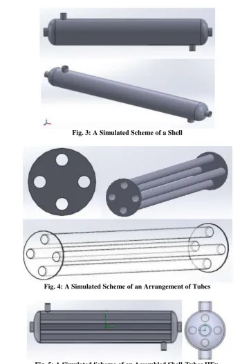
Using a derived dimensions (in Table.1) of shell-tubes HEx. shown in Fig.(2) create software model using flow simulation of SolidWorks® Premium 2014 edition. The parts individually as well as in assembly are as shown in Figs.(3-5).
Fig. 3: A Simulated Scheme of a Shell
Fig. 4: A Simulated Scheme of an Arrangement of Tubes
B. Input Physical Domains and Boundary Conditions
Here locating fluid domains on the model HEx., then applied the boundary conditions loads on the various faces and edges of the overall assembly. The boundary condition loads applied are shown in Fig.(6).
Fig. 6: A Simulated Scheme of the Loaded Boundary Conditions
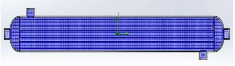
C. Mesh Generation and Steady State Thermal Simulation
This is the final and the most important step of analysis. The mesh has been generated to perform finite element analysis. In generating the mesh a compromise between computer speed and mesh quality has been adopted. The generated mesh along with its information has been shown in Fig.(7).
Fig. 7: A Simulated Scheme of the Generated Mesh Along
Then, the created model of shell and tubes heat exchanger exactly of the above derived dimensions is solved out under steady state thermal simulation. The results obtained were quite familiar with general considerations about the hierarchical nature of temperature, pressure, and void fraction profiles and turbulence zones of flow in tubes of a heat exchanger.
V.
RESULTS & DISCUSSION
A. Experimental Results
A number of verification runs were undertaken prior to the data logging. A series of tests for single-phase water flow were conducted to establish the validity of the system and test technique. All observations for the flow pattern by leaving the liquid flow rate fixed, flow patterns were observed for various air flow rates. The liquid flow rate was then adjusted and the process was repeated. All of the observed data points (6 points) were repeated four time to ensure of measurement. Then, evaluate U by using Eqn.(10) as a function of superficial Reynolds number of cold water (ReSL) and air (ReSG) [14]:
𝑅𝑒𝑆𝐿 = 𝜌𝑤𝑢𝑜𝐿𝑑𝑖
𝜇𝑤 ………….. (11)
𝑅𝑒𝑆𝐺 = 𝜌𝑔𝑢𝑜𝑔𝐷
𝜇𝑔 ………….. (12) where;
𝜌𝑤 : Density of water, (kg/m3)
di : Inside diameter of test tube section of a heat exchanger, (m) 𝑢𝑜𝐿 : Superficial average velocity of water in the test tube section, (m/s).
𝜇𝑤 : Viscosity of water at average temperature, (kg/m.s).
𝑢𝑜𝑔 : Superficial average velocity of air in the test tube section of steel pipe, (m/s).
D : Inside diameter of test tube section of steel pipe, (m)
𝜇𝑔 : Viscosity of water at average temperature, (kg/m.s).
The measurements in two-phase flow were performed for different air–water flow regimes. The water superficial velocity changed in the range from 0.035 to 0.213 m/s while the air superficial velocity varied from 0.7 to 3.14 m/s. The uncertainty of the temperature and pressure drop measurements in tubes-side were ranged ±(0.0328-0.206oC) and ±(0.037-1.36mmHg) respectively forquadruplicate replicate measurements of heat exchanger.
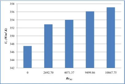
The overall heat transfer coefficients through heat exchanger between one phase (hot water) and two phase flow (mixture of cold water/air) are illustrate in Figs.(8-10). The main behavior for each one are shown that, overall heat transfer coefficient increase due to appears air with water flow, this reveals to increase of turbulence through tubes leading to decrease thickness of boundary layer inside tubes. An increase percent of the overall heat transfer coefficient for ReSL =651.05 reaches to (1.55, 1.87, 2.48, and 2.77%) for ReSG values (2692.7,
4071.37, 9499.86, and 10867.75) respectively. While for ReSL= 1953.14, percent reach (4.78 and 7.28%)
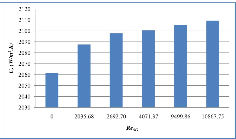
respectively, and for ReSL=3906.28 percent increase reach to (1.25, 1.76, 1.88, 2.13, and 2.32%) for ReSG values
(2035.68, 2692.7, 4071.37, 9499.86, and 10867.75%) respectively. This behaviour described in Figs.(8-10) reveals to that, the overall heat transfer coefficients increase in two-phase of the gas Reynolds number increased for a fixed ReSL in HEx. Generally increased as the air flow rate was increased for each fixed liquid flow rate.
Also, the increase in U was more significant at low ReSL than at high ReSL due to at low liquid flow rates, the
turbulence level in the liquid stream is small before being introduced into the gas stream. The introduction of the gas phase into the liquid stream increases the turbulence level which results in a high overall heat transfer coefficient. However, at high ReSL the turbulence level is already high and the effect of the gas-phase on U is
not that pronounced.
Fig. 8: Comparison of Overall Heat Transfer Coefficient vs. Air Reynolds Number at
Constant Liquid Flow Rate (ReSL=651.05)
342 344 346 348 350 352 354 356 358
0 2692.70 4071.37 9499.86 10867.75
U,
(
W/m
2.K
)
Fig. 9: Comparison of Overall Heat Transfer Coefficient vs. Air Reynolds Number at
Constant Liquid Flow Rate (ReSL=1953.14)
Fig. 10: Comparison of Overall Heat Transfer Coefficient vs. Air Reynolds Number at
Constant Liquid Flow Rate (ReSL=3906.28)
Also, comparison of the overall heat transfer coefficients estimated by using NTU-method in the current study are approximately comparable with that estimated by using a Log Mean Temperature Difference (LMTD) method that discussed by Maraie et al. [9]for the same range of ReSG and ReSL. The differences percent
were low for a fixed value of ReSL =651.05 were (1.63, 1.69, 4.38, and 4.36%) for ReSG values (2692.7, 4071.37,
9499.86, and 10867.75) respectively. While for ReSL= 1953.14, percent reach (1.64 and 1.54%) respectively, and
for ReSL=3906.28 percent decrease reach to (0.54, 0.12, 0.03, 0.1, and 0.003%) for ReSG values (2035.68, 2692.7,
4071.37, 9499.86, and 10867.75%) respectively. These low deviation between results of both methods indicate to the efficient use of both methods to analysis of heat exchangers with a high accuracy.
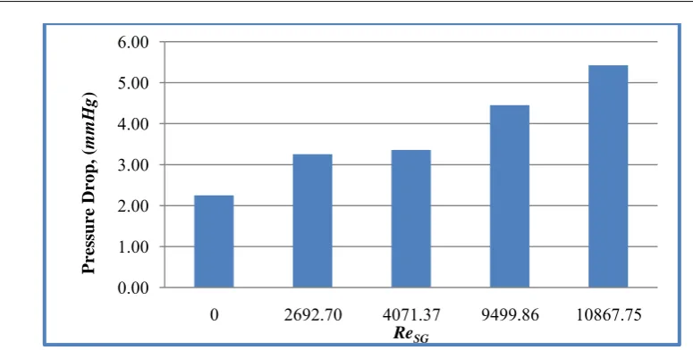
Comparison of the pressure drop of heat exchanger between one phase (cold water) and two phase flow (cold water/air mixture) are illustrate in Figs.(11-13). The main behavior for each one are shown that, pressure drop through pipe side increase due to appears air with water flow, this reveals to increase of turbulence through tubes leading to increase the pressure drop through tubes as discussed by Maraie et al. [9].
960 980 1000 1020 1040 1060 1080 1100
0 9499.86 10867.75
U,
(
W/m
2.K
)
ReSG
2030 2040 2050 2060 2070 2080 2090 2100 2110 2120
0 2035.68 2692.70 4071.37 9499.86 10867.75
U,
(
W/m
2.K)
Fig. 11: Comparison of Tubes Pressure Drop vs. Air Reynolds Number at
Constant Liquid Flow Rate(ReSL=651.05)
Fig. 12: Comparison of Tubes Pressure Drop vs. Air Reynolds Number at
Constant Liquid Flow Rate (ReSL=1953.14)
Fig. 13: Comparison of Tubes Pressure Drops vs. Air Reynolds Number at
Constant Liquid Flow Rate (ReSL=3906.28)
0.00 1.00 2.00 3.00 4.00 5.00 6.00
0 2692.70 4071.37 9499.86 10867.75
P re ss ure Dro p, ( m m H g ) ReSG 0.00 5.00 10.00 15.00 20.00 25.00 30.00 35.00 40.00
0 9499.86 10867.75
P re ss ure Dro p, ( m m H g ) ReSG 0.00 20.00 40.00 60.00 80.00 100.00 120.00 140.00 160.00 180.00 200.00
0 2035.68 2692.70 4071.37 9499.86 10867.75
B. Simulation Results
The simulations were carried out as 3-D for one phase (cold water) and, two-phase (air-cold water) flow in a shell-tubes HEx. based on Turbulence Intensity and Length (I-L) model, and solved in a flow simulation of SolidWorks premium 2014. Residual converged, the solutions are extracted and the obtained results are illustrated by figures able to capture the main features of the flow with heat transfer in shell-tubes heat exchanger. Several simulations were carried out using progressively larger number of grid points, until practically no change in the liquid velocity profiles was observed beyond a finite number of grids. At the pipe inlet, uniform liquid velocity, temperature, and turbulence intensity have been specified; a relative average static pressure of zero was specified at the pipe outlet. No slip boundary conditions were used at wall. Convergence criterion used was 1.0*10−5 for all the equations except for energy equation was 1.0*10−9.
1) One-Phase Flow:At the tubes side inlet, uniform gas and liquid velocities, temperature, and turbulence intensity have been specified; a relative average static pressure of zero was specified at the tubes outlet. No slip boundary conditions were used at wall. Average uniform liquid velocity profile are specified for initiating the numerical solution. In this analysis, a superficial velocity in tubes ranged between 0.035-0.212m/s for cold water at the inlet are specified. For the heat transfer cases, hot fluid water at 325 K enters at the top of the HEx..
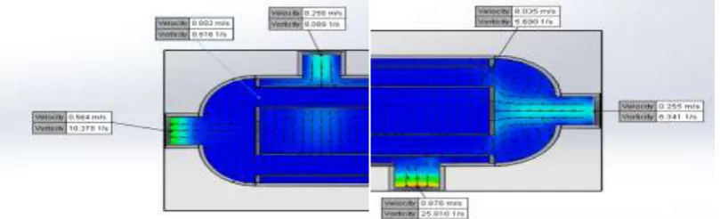
Velocity distributions in shell and tubes HEx. for basic design is shown in Fig.(14), for a single phase flow of a cold water in tubes. The average inlet velocity into the tubes is 0.035 m/s then decrease gradually along the length of tubes to exit at 0.002 m/s, due to the loses by friction with wall of tubes. The highest velocity of flow occurs at the inlet section of tubes then the velocity developing to reach a fully homogeneous distribution of turbulence at endings part of tubes. In contrast the average inlet velocity into the tubes side was 0.255 m/s side due to the load of pressure acts by pump then exit from tubes side at 0.564 m/s.
Fig. 14: Contours of Average Velocity DistributionsatConstant Liquid Flow Rate(ReSL=651.05)
The turbulence distributions of the inlet and outlet water in shell and tubes are shown in Fig.(15), in which the inlet tubes velocity was 0.035 m/s, as presented the vorticity distribute in a high value at inlet zone of tubes (5.69 1/s) then continue of mixing the fluid to developing then reach a homogeneity distribution at outlet zone with decreasing of the average velocity (0.002 m/s) as a result of drag forces due to friction with a tubes wall. Also note that a decreasing of vorticity as a result of the fully developing of a homogeneous turbulence distribution.
Fig. 15: Turbulence Distributions of Inlet & Outlet Water in Shell & Tubes
The contour of temperature is shown in Fig.(16). Contours of temperature can explain performance of HEx. clearly. Certainly temperature’s profiles are derived flow’s profiles. Using contours of temperature that are exhibited graphically, the analysis of temperature differences in HEx. length is possible.
Fig. 16: Contours of Temperatures Distributions at Constant Liquid Flow Rate(ReSL=651.05)
As shown in the outlet temperature recorded by a simulation of the tubes zone is about 305.80K, while it recorded experimentally about 305.84 K in tube-side, and for shell-side was about 318.07 K while experimentally was 316.75 K. These results indicate the compatibility of simulation models for heat exchanger with a laboratory model.
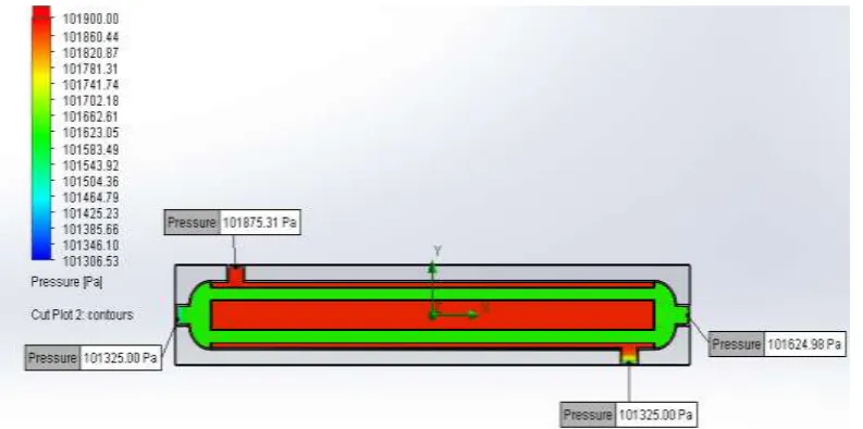
The pressure distribution through a HEx. is shown in Fig.(17), whereas there is no great difference between input and output points due to a used HEx. with a small size, and a low flow rate used in run of the experiments. But in general, there is a good agreement of values of pressure drops between both of simulated and experimental values as shown in Table 2.
Fig. 17: Contours of Pressure Distributions Through a HEx. at Constant Liquid Flow Rate(ReSL=651.05)
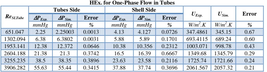
between 0.0013-0.389%. It have great values compared to shell-side, due to a small diameter of used tubes with respect to a shell-side diameter.
Table 2.Comparison Between Experimental and Simulation Results of a Shell-Tubes HEx. for One-Phase Flow in Tubes
ReSLTube
Tubes Side Shell Side
UExp. USim. Error
∆PExp. ∆PSim. Error ∆PExp. ∆PSim. Error
mmHg mmHg % mmHg mmHg % W/m2.K W/m2.K %
651.047 2.25 2.25003 0.0013 4.13 4.127 0.0726 347.4861 345.15 0.67 1302.094 6.38 6.3802 0.0031 5.88 5.89 0.1701 693.4115 689.24 0.60 1953.141 12.38 12.372 0.0646 10.38 10.356 0.2312 1003.071 998.78 0.43 2604.188 21.38 21.3 0.3742 16.5 16.39 0.6667 1349.68 1345.79 0.29 3255.235 38.5 38.35 0.3896 23.63 23.58 0.2116 1725.74 1721.66 0.24 3906.282 55.63 55.44 0.3415 37.88 37.74 0.3696 2061.567 2057.32 0.21
2) Two-Phase Flow:At the tubes side inlet, uniform gas and liquid velocities, temperature, turbulence intensity and average volume fractions have been specified; a relative average static pressure of zero was specified at the pipe outlet. No slip boundary conditions were used at wall. Average mass fraction and uniform liquid velocity profile are specified for initiating the numerical solution. Convergence criterion used was 1.0*10−5 for all the equations except for an energy equation was 1*10-9. In this analysis, a superficial velocity in tubes ranged between 0.035-0.212m/s for cold water, and 0.0002-0.002 mass fraction of air at the inlet are specified. For the heat transfer cases, hot fluid water at 325 K enters at the top of the HEx.
Velocity distribution in shell and tubes HEx. for basic design is shown in Fig.(18) for a two phase flow of an air/cold water in tubes. The average inlet velocity into the tubes is 0.286 m/s then decrease gradually along the length of tubes to exit at 0.024 m/s, due to the loses occur by friction with wall of tubes. The highest velocity flow occurs at the inlet section of tubes with great vorticity value (27.472 1/s) then the velocity developing to reach a fully homogeneous distribution of turbulence at endings part of tubes with low average velocity (0.024
m/s) and small value of vorticity (2.703 1/s). In contrast the average inlet velocity into the tubes side was 1.68
m/s due to the load of pressure acts by pump then exit from tubes side at 1.777 m/s.
As shown in Fig.(18) the average inlet velocity of two phase flow (0.286 m/s) was greater than of one phase flow that shown in Fig.(14) it's about (0.035 m/s), due to presence of air that leading to increasing the turbulence and vorticity through tubes of a HEx.
Fig. 18: Contours of Average Velocity Distributionsat Constant Flow Rates
(ReSL=651.05 and ReSG=2692.70)
Fig. 19: Contours of Temperatures Distributionsat Constant Flow Rates
(ReSL=651.05 and ReSG=2692.70)
As shown in the outlet temperature recorded by a simulation of the tubes-side is about 305.94K, while it recorded experimentally about 305.98 K in tubes-side, and for shell-side was about 317.33 K while experimentally was 316.75 K. These results indicate the compatibility of simulation models for heat exchanger with a laboratory model.
The local air void fractions and their variation along the tubes for the two-phase flow condition are shown in Fig.(20). The temperature, and velocity distributions appear clearly along the tubes at the same sites that have high uniform turbulence and low vorticity as shown in Figs. (19 & 20). That reveal a type of the flow’s distribution is effective parameter of heat exchangers rate of heat transfer, whereas the relatively low flow rates in tubes for highest void fractions occurring in that area. It is noteworthy that while flow mixing and heat transfer are enhanced upstream of the tubes, void fractions are higher locally on the downstream side as a result of wake turbulence and stagnation as shown in Fig.(20).
Fig. 20: Contours of Mass Fraction Distributions of Mixture (Air-Cold Water) in Tubes
at Constant Flow Rates(ReSL=651.05 and ReSG=2692.70)
The pressure distribution through a HEx. is shown in Fig.(21), whereas there is no great difference between input and output points along tubes due to a used HEx. has a small size, and low flow rate used in run of the experiments. In general, there is a good agreement of values of pressure drops between both of simulated and experimental values as shown in Table 3.
Fig.21: Contours of Pressure Distributions Through a HEx.at Constant Flow Rates
Table 3 represent a comparison of the overall heat transfer coefficients obtained by using (I-L) model, and experimental values.
Table 3. Comparison between Experimental and Simulation Results of a Shell-Tubes HEx. for Two-Phase Flow in Tubes
ReSGTube ReSLTube
Tubes Side Shell Side
UExp. USim. Error
∆PExp. ∆PSim. Error ∆PExp. ∆PSim. Error
mmHg mmHg % mmHg mmHg % W/m2.K W/m2.K %
2692.70 651.05 3.25 3.26 0.308 4.13 4.128 0.048 352.89 350.72 0.615 4071.37 651.05 3.36 3.33 0.893 4.13 4.123 0.169 354.00 351.89 0.596 9499.86 651.05 4.45 4.42 0.674 4.13 4.126 0.097 356.12 354.14 0.556 10867.75 651.05 5.43 5.39 0.737 4.13 4.127 0.073 357.12 355.21 0.536 9499.86 1953.14 28.80 28.58 0.764 10.38 10.36 0.193 1051.06 1044.25 0.648 10867.75 1953.14 34.02 33.75 0.794 10.38 10.36 0.193 1076.16 1072.69 0.322 2035.68 3906.28 93.98 93.2 0.830 37.88 37.75 0.343 2087.54 2075.75 0.565 2692.70 3906.28 97.65 96.83 0.840 37.88 37.75 0.343 2097.83 2074.23 1.125 4071.37 3906.28 107.32 106.3 0.950 37.88 37.75 0.343 2100.48 2119.58 0.910 9499.86 3906.28 148.80 147.34 0.981 37.88 37.75 0.343 2105.52 2088.96 0.786 10867.75 3906.28 176.98 175.23 0.989 37.88 37.75 0.343 2109.37 2091.2 0.861
Results predicted by simulations illustrate that the turbulent intensity increases as the flow passed through tubes. The increased turbulent intensity helps improving the rate of heat transfer in the heat exchanger. Generally the overall heat transfer coefficients of two-phase flow are greater than the heat transfer coefficients of the one-phase flows.A comparison of the overall heat transfer coefficients show that, there is a good agreement between both of experimental and the simulated results. It is been predicted compatibility by this model with an average error of 0.322-1.125%. The good thing about these results is the constant difference from experimental results and consistency with the real systems, i.e. with higher pressure drop, higher heat transfer is achieved. Therefore, it could be state that type of the flow’s distribution is effective parameter in HEx’s rate of heat transfer and consequently in heat recovery quantity of it. Also, the pressure drop in shell and tubes sides are presented in Table 3, in which the pressure drop in the shell is under-predicted by the (I-L) model by almost 0.048-0.343%. As well the pressure drop in tube side (straight tubes) is predicted with an average error between 0.308-0.989%. The two-phase flow effects on pressure drop is captured by the CFD model for the full range of exit qualities. The two-phase flow effect on pressure drops is more pronounced for the CFD results compared to the experimental data. This discrepancy may indicate inaccurate wall heat transfer and bubble departure modeling that gives rather unrealistic void development along the channel [15].
VI.
CONCLUSIONS
Single and two-phase flow RANS CFD simulations were performed for the shell-tubes heat exchangers. A three-dimensional turbulent flow structure and the heat transfer performance of the shell-tubes heat exchanger have been investigated. Results predicted for both single and two-phase are in good agreement overall with the test data, and the for main flow features at known exit qualities was captured by the CFD model similar to the patterns observed in the Labs experimental data.The predicted by simulations of velocity, temperature, and pressure drops distributions illustrate that the turbulent intensity increases as the flow passed through tubes due to presence of a dispersed air that leading to induced strong vortices. However, the increased turbulent intensity helps to reducing a flow resistance as a result of adding a dispersed air and improving the rate of heat transfer. So, the developed CFD methodology is useful for understanding the flow behavior and predicting main flow features effect on thermal hydraulic performance of shell-tubes HEx.
REFERENCES
[1]. V.P. Dubey, R.P. Verma, P.S. Verma, and A.K. Srivastava, "Steady State Thermal Analysis of Shell and Tube Type Heat Exchanger to Demonstrate the Heat Transfer Capabilities of Various Thermal Materials using Ansys", Global Journal of Researches In Engineering, Vol. 14(4), 2014.
[2]. S. Lin, J. Broadbent, and R. McGlen, "Numerical study of heat pipe application in heat recovery systems", Applied Thermal Engineering, Vol. 25, pp.:127-133, 2005.
[3]. M.H. Saber, and H.M. Ashtiani, "Simulation and CFD Analysis of heat pipe heat exchanger using Fluent to increase of the thermal efficiency", In Proceedings of 5th IASME/WSEAS International conference on Continuum Mechanics, Vol. 183, 183-189, 2010.
[5]. P. Patel, and A. Paul, "Thermal Analysis of Tubular Heat Exchanger by Using Ansys", International Journal of Engineering Research & Technology, Vol. 1(8), pp.: 1-8, 2012.
[6]. A. Gopi Chand, A.V.N.L. Sharma, G. Vijay Kumar, and A. Srividya, “Thermal Analysis of shell and tube heat exchanger using MATLAB and FLOEFD software”, International Journal of Engineering Research & Technology, Vol. 1(11), pp.: 3276 –3281, 2012.
[7]. E. Ozden, and I. Tari, “Shell side CFD analysis of a small shell-and-tube heatexchanger”, Energy Conversion and Management, Vol. 51(5), pp.: 1004 – 1014,2010.
[8]. M. R. Rahimi, A. Askari, and M. Ghanbari, "Simulation of Two Phase Flow and Heat Transfer in Helical Pipes", 2nd International Conference on Chemistry and Chemical Engineering (IPCBEE), Vol.14, pp.: 117-121, 2011.
[9]. A.A. Maraie, A.A.M. Hassan, M.S. Hassan, T.E.M. Farrag, and M.M. Nassar, "An Investigation of Heat Transfer for Two-Phase Flow (Air-Water) in Shell and Tubes Heat Exchanger", International Journal of Innovative Research in Science, Engineering and Technology, Vol. 5(1), pp.: 414-427, 2016. [10]. W.M. Kays, and A.L. London,Compact heat exchangers: a summary of basic heat transfer and flow
friction design data, National Press, 1955.
[11]. Cengel Y.A., Heat Transfer: A Practical Approach, 2nd edition, McGraw-Hill, 2003. [12]. J.P. Holman, Heat Transfer, 8th ed., McGraw-Hill, 2001.
[13]. F.P. Incropera, and D.P. DeWitt, Fundamentals of Heat and Mass Transfer, 4th Edition, John Wiley & Sons, 1996.
[14]. D. Kim, “Heat Transfer Correlations for Air-Water Two-Phase Flow of Different Flow Patterns In a Horizontal Pipe”, KSME International Journal, Vol.15(12), pp.: 1711-1727, 2001.