Abstract—This paper proposes a new approach for solving the complicated environmental protection power dispatch (EPPD) problem for modern power system. In the work, pollutant emission and generation cost, which are two conflicting objective functions, are taken into account concurrently within the optimization process. Then, the proposed interactive bi-objective programming with valuable trade-off (IBPVT) approach is applied to obtain an pareto-optimal solution, which is an emission-cost trade-off solution, by following the intention of the decision maker. The salient feature of the proposed approach is that it can provide a flexible and compromising solution through an easy and interactive process to help power systems obtain the optimal emission-cost power dispatch. Two test cases have been demonstrated and proven to obtain the superior features. The encouraging simulation results show that the proposed approach is capable of obtaining high quality solutions for practical EPPD problems.
Index Terms—Environmental protection power dispatch, interactive bi-objective programming with valuable trade-off, pareto-optimal solution.
I. INTRODUCTION
The rising awareness about environmental protection has forced modern power systems to remedy their operation strategies for reducing pollutant emission of thermal generation units. Since power dispatch is the fundamental issue during the operation process, it should be an attractive concern to take both emission and generation cost into account. A survey of the literature on power dispatch indicates that various methods have been proposed for solving the environmental protection power dispatch (EPPD) problem [1]-[7]. In the authors’ previous effort, a single objective programming approach, in which the emission was treated as a constraint within a permissible limit, was developed to solve the EPPD problem [2]. However, the single objective programming method has the problem of requiring the trade-off relations between generation cost and emission. In another research direction, the bi-objective
Manuscript received March 29, 2013. This work was supported in part by the National Science Council of the Republic of China, Taiwan, under Grant NSC-97-2221-E-129-020-MY3.
Po-Hung Chen and Feng-Jih Wu, and Li-Ming Chen are with the Department of Electrical Engineering, St. John’s University, New Taipei City, 25135 Taiwan (e-mail: [email protected]; [email protected]; [email protected]).
Hung-Cheng Chen is with the Department of Electrical Engineering, National Chin-Yi University of Technology, 41107 Taichung, Taiwan (e-mail: [email protected]).
An Liu is with the Department of Computer Science and Information Engineering, St. John’s University, New Taipei City, 25135 Taiwan (e-mail: [email protected]).
power dispatch problem was converted to a single objective problem by linear combination of the different objectives through weighted values [3], [4]. However, the units of the different objective functions may be different. Moreover, there is no direct corresponding transformation relationship, meaning that weighted values cannot be used to represent the importance of different objective functions. Hence, it is difficult to determine the weighted value using intuition. Obviously, a complete and efficient approach for solving the EPPD problem is still required.
Recently, multi-objective algorithms have also been used to solve the EPPD problem [1], [5]-[7]. Since these algorithms search a population of candidate solutions instead of a single candidate solution during the solution process, multiple solutions can be found in one single run. However, electric utilities usually prefer the simple and interactive EPPD software to provide the best compromise solution rather than a set of solutions. Therefore, a new bi-objective formulation combined with the developed IBPVT method is proposed in this paper.
A global optimization technique called particle swarm optimization (PSO) [8], [9] has been used to solve real time issues and aroused researchers' interest due to its flexibility and efficiency. Limitations of the classic greedy search technique, which restricts allowed forms of fitness functions, as well as continuity of the variables used, can be entirely eliminated. Our previous work on PSO approach [10] is applied in this paper as a solution tool for the IBPVT approach. The feasibility of the proposed method was demonstrated on two different systems and then compared with the real-coded PSO, GA, and evolutionary algorithm methods regarding solution quality and computational efficiency.
II. PROBLEM FORMULATION A. List of Symbols
i
P : output energy of generator i for dispatched hour,
) (⋅
i
F : generation cost function of generator i, )
(⋅ i
E : Emission function of generator i,
i a bici
i e fi
: coefficients of the generation cost functions for generator i, considering valve-point effects,
i
α βiγi i
ζ λi
: coefficients of the emission functions for generator i,
D
P : energy demand for dispatched hour,
L
P : transmission network losses of system,
ij
B : B coefficients for loss calculation,
Environmental Protection Power Dispatch for Modern
Power System
pre i
P : output energy of generator i before dispatched
hour,
i
UpR : up ramp limit of generator i,
i
DownR : down ramp limit of generator i, max
i
P : maximum energy output limit of generator i,
min
i
P : minimum energy output limit of generator i, lower
j i
PZ, : lower bound of the j-th prohibited zone for generator i,
upper j i
PZ, : upper bound of the j-th prohibited zone for generator i,
i
PZ : number of prohibited zones for generator i,
Cost : cost function for optimization approach,
i
NP : normalized power output of generator i,
Fitness : fitness function for PSO, applied on power dispatch,
w : weight factor for fitness function, Obj
N_ : normalized Obj, min
Obj : minimum Obj value of initial generation, max
Obj : maximum Obj value of initial generation,
PB : penalty function for power balance constraints. B. Objective Functions
The objective of power dispatch problem is to minimize two competing objective functions, total generation costs and emission of a power system over an appropriate period (usually one hour), while satisfying several equality and inequality constraints. Due to the highly non-linearity characteristics of power systems and generators, power dispatch belongs to a class of bi-objective nonlinear programming optimization containing equality and inequality constraints as stated below:
1)Generation cost
Generally, the generation cost function is usually expressed as a quadratic polynomial. However, it is more practical to consider the valve-point effects for fossil-fuel-based plants. Therefore, the cost function considered in this paper can be represented as below:
F Pi( )i = +ai b P c Pi i+ i i2+ ×ei sin( (f Pi imin−Pi)) (1) 2)Emission
The total emission in (ton/h) of atmospheric pollutants such as sulpher oxides and nitrogen oxides caused by the operation of fossil-fueled thermal generation can be expressed as
( ) 2 i iP
i i i i i i i i
E P =α β+ P+γ P +ζ eλ (2)
C.Constraints
The available operating range of generators is restricted by their mechanical and electrical characteristics, such as ramp rate limits, prohibited zones, and bounded power output. These practical constraints to generator operations must be taken into account to achieve effective power operations.
1)Power balance
The total power output of generators must be always equal the sum of the power demands and the network losses, as expressed in (3).
1
m
i D L
i
P P P
= = +
∑
(3)Since power plants are spread out geographically, transmission network losses should be taken into account. To calculate network losses, the B coefficient method is commonly used by the power utility industry. It can be expressed as a quadratic function, as shown in (4).
0 00
1 1 1
m m m
L i ij j i i
i j i
P P B P B P B
= = =
=
∑∑
+∑
+ (4)2)Ramp rate limits
The power output of a practical generator cannot be adjusted instantaneously without limits. The operating range of all on-line units is restricted by their ramp rate limits during each dispatch period. Therefore, the subsequent dispatch output of a generator should be limited between the constraints of up and down ramp rates, as shown in (5). pre pre
i i i i i
P −DownR ≤ ≤P P +UpR (5) 3)Prohibited operating zone and generation limits
Each generator has its generation capacity, which cannot be exceeded at any time. Moreover, a typical thermal unit may have a steam valve in operation, or a vibration in a shaft bearing, which may result in interference and discontinue input-output performance-curve sections, called prohibited zones. Therefore, in practical operation, adjusting the power output of a unit must avoid all capacity limits and unit operations in prohibited zones. The feasible operating zones of a unit can be described as follows:
min
,1
, , 1
max ,
, 2,3,..., i
lower
i i i
upper lower
i i j i
i j upper
i i
i PZ
P P P
P P P j PZ
P P P
−
⎧ ≤ ≤
⎪ ⎪
≤ ≤ =
⎨ ⎪
≤ ≤ ⎪⎩
(6)
The main objective of power dispatch is to minimize the total generation cost and emission of specific operating intervals, while satisfying all inequality/equality constraints, as stated below:
1
1 ( ) min
( ) m
i i i m
i i i
Total Fuel Cost F P
Total Emission E P
=
=
⎧
= ⎪
⎪ ⎨
⎪ =
⎪⎩
∑
∑
subject to (3), (5) and (6)III. THE IBPVT APPROACH
This paper proposes the IBPVT approach which uses a simple interactive method to satisfy users’ preferences and obtains the more valuable trade-off pareto-optimal solution for the bi-objective function. In the solving process, users do not need to input a weighted value, but only need to make a choice of favorite objective function and the bi-objective problem can be solved smoothly. The main advantage of this method is in providing a larger programming space in the modeling process which is not limited to a single objective programming model. The problems of bi-objective programming can be easily solved so as to provide users with more favorable solutions and a more convenient operating environment.
A. Theoretical Interpretation
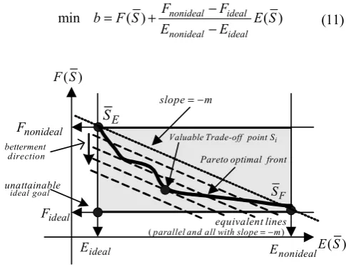
Assume the bi-objective function to be solved is shown as (8). The pareto-optimal front of this bi-objective function (8) is shown as the thick solid line in Fig. 1. SE is the single objective optimal solution when considering only objective function E(S); thus, the corresponding Eideal should be the
optimal value of E(S). Because the effect of F(S) is not considered, the corresponding Fnonideal should be the
non-ideal value of F(S). On the other hand, SF is the
single objective optimal solution when considering only the )
(S
F objective function; thus, the corresponding Fideal is the optimal value of S(S)and the corresponding Enonideal should be the non-ideal value of E(S). The solution that makes (E(S),F(S))=(Eideal,Fideal) is the unattainable ideal goal. Therefore, the proposed approach attempts to seek solution S, which is not only closer to the unattainable ideal goal (Eideal,Fideal) but also has the more valuable trade-off among pareto-optimal solutions in accordance with users’ requirements.
The slope of the straight line connecting SE and SF ,
shown in Fig. 1, is
ideal nonideal
ideal nonideal
E E
F F
m
− − −
=
− . Here, m
represents the average trade-off ratio between these two objective functions.
) (S F
) (S E ideal
E Enonideal
nonideal
F
ideal
F
1 E 1
F
E
S
F
S m
slope=−
1
P
front optimal Pareto
2
E
2 F
2
P
advance
F
expense
E b
ideal goalle unattainab
Fig. 1. Theoretical interpretation of bi-objective programming. For pointP1, as shown in Fig. 1, the corresponding values
of E(P1) and F(P1) are E1 and F1, respectively. With the bi-objective optimization concept, there would be no advantage between P1 and P2, since P2 has Fadvance with the deterioration of Eexpense where the ratio of advance and expense is the same as with the average trade-off ratio m. Therefore, P2 is located in a line that has the same slope as that which forms SE and SF , so that:
1 2 2 1 exp
advance nonideal ideal
ense nonideal ideal
F F F
F F
m
E E E E E
−
− = = =
− − (8)
1
P and P2 determine a line that has slope −m and intercept b in F(S) axis. All of the points in this line will have similar conceptual performance for bi-objective programming based on mathematical explanation. The line equation can be formulated as below:
( ) ( ) nonideal ideal ( )
nonideal ideal
F F
F S mE S b E S b
E E
−
= − + = − +
− (9)
( ) nonideal ideal ( )
nonideal ideal
F F
b F S E S
E E
−
= +
− (10) The solution S that caused a smaller b in (10) represents a better result because it is closer to the unattainable ideal goal. Therefore, to find a solution S that can have min b
will be a more valuable trade-off solution of bi-objective programming, as shown in Fig. 2. The valuable trade-off solution for bi-objective programming is then formulated as below:
min ( ) nonideal ideal ( )
nonideal ideal
F F
b F S E S
E E
−
= +
− (11)
) (S F
) (S E ideal
E Enonideal
nonideal
F
ideal
F equivalentlines
E
S
F
S m
slope=−
front optimal Pareto
) (parallelandallwithslope=−m
le unattainab
goal ideal
i S point Trade-off Valuable betterment
direction
Fig. 2. Valuable trade-off point of bi-objective programming. However, if the decision maker still have a preference for the dedicated objective, it only needs straightforward consideration of the percentage of favorites objective with a simple weight w. Suppose the decision maker thinks that F
is more important than E for the final result, for example 80%
'
exp
(1 ) 1 1
advance nonideal ideal
ense nonideal ideal
w F w w F F
m m
w E w w E E
× −
= = = ×
− × − − −
(12) A similar formulation process as (8) to (10) then changes the bi-objective programming, as below, to take decision maker’s willing into consideration easily:
min ( ) ( )
1
nonideal ideal nonideal ideal
F F
w
b F S E S
w E E
−
= +
− − (13)
B. Solution Procedure of IBPVT
According to the discussion above, the solving process of the IBPVT method is divided into three steps and shown as follows.
1)Step 1:
Solve single objective functions (14) and (15) below to get SE , Eideal , Fnonideal and SF , Fideal , Enonideal , respectively.
min ( ) subject to all constraintsE S (14)
min ( ) subject to all constraintsF S (15) 2)Step 2:
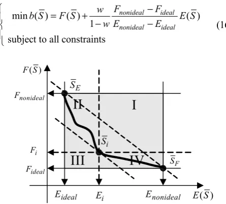
Solve objective function (16), as below, to get the valuable trade-off solution that should satisfy all constraints. Suppose that Si is solved, as shown in Fig. 3.
min ( ) ( ) 1 ( )
subject to all constraints nonideal ideal nonideal ideal
F F
w
b S F S E S
w E E
− ⎧
= +
⎪ − −
⎨ ⎪ ⎩
(16)
) (S F
) (S E
ideal
E Enonideal
nonideal
F
ideal
F
i
E
i
F Si
I
IV
III
II
E
S
F
S
Fig. 3. Solution space of IBPVT after Si is solved.
The Si divides the shaded part in Fig. 3 into areas I, II, III and IV. Area III can be called the “unreachable solution space” since no solutions could be obtained in this area. The solutions in area I are even worse than Siso there is no need to consider this area. The pareto-optimal front in area II possesses one characteristic in which E(Area_II) is superior to Ei but F(Area_II)is worse thanFi. Similar situations also occur in area IV. This characteristic can help users searching for preferred solutions when considering different policies to be processed in the next step.
3)Step 3:
To reach an interactive relation with users, if the decision maker is not satisfied with Si in Step 2, one objective
function may be compromised to improve another objective function as follows. If the intention is to further improveE(S), Ei obtained in Step 2 is regarded as the newEnonideal, and Fi is considered as the new Fideal, as shown in (17). The corresponding solution space is reduced to area II and Step 2 is repeated to find the valuable trade-off solution within the preferred boundary, as shown in Fig. 4. On the other hand, if the intention is to further improveF(S),
i
F obtained in Step 2 is regarded as the new Fnonideal and i
E is considered as the new Eideal.
nonideal i ideal i
E E
F F
= ⎧
⎨ =
⎩ (17)
) (S F
) (S E ideal
E Enonideal
nonideal
F
ideal
F
i
E i
F
i
S E
S
F
S Dis_E
Dis_F
Fig. 4. Solution of IBPVT after improving E(S).
As shown from the above discussion, solving direction conforms to users’ requirements. Users only need to input the objective function intended to be improved and the proposed approach can find a valuable trade-off solution meeting that requirement without considering any weighting value. As shown in Fig. 4, the whole space of feasible solution can automatically reduce its range according to decision maker’s requirements. Each time the search is done, the space gradually turns to the decision maker appointed direction. As each search may reduce the space of feasible solutions,
E
Dis_ and Dis_F provided in the research are shown in (18), as reference for determining the next search. As shown in Fig. 4, Dis_E and Dis_F in (18) represent the ranges of EandF , respectively, in space of feasible solution. If
E
Dis_ and Dis_F are too small, there will not be a significant difference of solution in the next search. Therefore, the next search may not be necessary. However, if
E
Dis_ and Dis_F remain large enough, there might be a different result in the next search that makes it worth doing. _
_
nonideal ideal nonideal ideal
Dis E E E
Dis F F F
= −
⎧
⎨ = −
⎩ (18)
need to choose a favorite objective function. It is unnecessary to consider the selection of weighting value or unit difference of objective functions. Thus, the work for decision maker is straightforward and solution efficiency can be effectively increased. The main advantage of IBPVT is in providing a larger programming space in the modeling process, as it is not limited to single objective programming. The problems of bi-objective programming can be easily solved so as to provide users with more favorable solutions and a more convenient operating environment.
The fitness function to evaluate each individual particle is formulated in (19). This function consists of the objective value and the power balance constraint shown in (20) and (21). If the values of N_Obj and PB for individual particles were small, then their Fitness value would be large to represent better solution. The weight factor w is set to 1 in our four test cases. However, w>1 could be given to maintain power balance constraint under the cases that N_Obj
dominates the Fitness value. 1
_
Fitness
N Obj w PB
=
+ × (19)
min
max min
( )
_ 1
( )
Objt Obj
N Obj abs
Obj Obj
− = +
− (20)
2 1
1 (m i D L)
i
PB P P P
=
= +
∑
− − (21)IV. TEST RESULTS AND DISCUSSION
The proposed approach was implemented using Matlab 7.0 and simulations were performed utilizing Intel Core2 Quad 2.0 GHz PC. To verify the feasibility and effectiveness of the proposed approach, two different examples were performed and their solution quality, convergence characteristics, and computational efficiency were compared with literature.
A. Simulation Cases and Results 1) Case 1
The IEEE 30-bus system [3], [5], [11] which consists of six units and 41 interconnected transmission lines, was tested and compared with GA and PSO approaches. The total load demand is 2.834 p.u. Generation cost and emission function coefficients along with each generator capacity limits can be found in [3], [5], [11]. Generation cost and emission functions were minimized individually using proposed approach, GA and PSO, see Table I. The proposed approach was also compared to those reported using linear programming (LP) [3] and multi-objective stochastic search technique [5], [12]. The comparison is shown in Table II.
As shown in Tables I and II, the applied PSO approach offers improved solutions over PSO, GA, some traditional
methods and multi-objective stochastic search techniques, clearly showing the ability of the proposed approach to reach better solutions quality. The results also confirm the potential of PSO algorithms to solve real-world highly nonlinear constrained optimization problems.
TABLEI: BEST GENERATION COST AND EMISSION OF PROPOSED APPROACH COMPARED TO PSO AND GA
Output (p.u.)
Single objective optimization
Proposed PSO method [11] GA method [5] Cost Emission Cost Emission Cost Emission P1 0.10972 0.40607 0.109922 0.402285 0.1095 0.4058 P2 0.29976 0.45907 0.299959 0.458427 0.2997 0.4592 P3 0.52430 0.53794 0.526262 0.540935 0.5245 0.5380 P4 1.01620 0.38295 1.014833 0.383863 1.0160 0.3830 P5 0.52430 0.53794 0.522898 0.538283 0.5247 0.5379 P6 0.35972 0.51003 0.360126 0.510206 0.3596 0.5101 Total
Output 2.834000 2.834000 2.834000 2.834000 2.834000 2.834000 Cost ($/h) 600.1114 638.2736 600.1118 637.9662 600.1114 638.2609 Emission 0.222145 0.194203 0.222037 0.194204 0.222143 0.194203
TABLEII:BEST GENERATION COST AND EMISSION OF PROPOSED APPROACH COMPARED TO TRADITIONAL ALGORITHMS Single
objective
Proposed LP [3] MOSST [12] Cost Emission Cost Emission Cost Emission Cost ($/h) 600.11 638.27 606.31 639.60 605.89 644.11
Emission 0.2222 0.1942 0.2233 0.1942 0.2222 0.1942 Single
objective
NSGA [5] NPGA [5] SPEA [5] Cost Emission Cost Emission Cost Emission Cost ($/h) 600.34 633.83 600.31 636.04 600.22 640.42
Emission 0.2241 0.1946 0.2238 0.1943 0.2206 0.1942
For each non-dominated solution, a normalized membership function (NMF) μk [5] for the selection of best compromised solution among Pareto-optimal set that found by multi-objective algorithms is calculated by (22).
1 1 1
obj
obj
N k i
k i
N M
j i j i
μ μ
μ =
= =
=
∑
∑ ∑
(22)
min
max
max min max min
max
1
0
i i
i i
i i i i
i i
i i
F F
F F
F F F
F F
F F
μ
⎧ ≤
⎪
⎪ −
=⎨ ≤ ≤
− ⎪ ⎪
≥ ⎩
(23)
values of the i-th objective function, respectively. The best compromise solution is the one having the maximum ofμk.
The proposed approach and other multi-objective search methods are applied to the problem and both objectives were treated simultaneously as competing objectives. Their best compromised solutions that chose from pareto-optimal set according to the NMF are shown in Table III. It is obvious that the proposed approach can provide a better compromised solution that with higher NMF than the other methods. The main reason is that the proposed approach focuses on searching the valuable trade-off solution instead of pareto-optimal set. Although, the proposed approach can not offer a set of pareto-optimal solutions in a single run like could do. However, the decision maker usually prefers the operational software to provide one best compromised solution from pareto-optimal solutions. Hence, the proposed approach can deal with this requirement directly and precisely.
There might be unsuitable about the first provided valuable trade-off solution due to the decision maker’s specially concern. The proposed approach provides the interactive process to help the decision maker for finding suitable and valuable trade-off solution automatically and easily. The test results for showing this salient feature are summarized in Table IV. The satisfaction rates for both the generation cost and emission are defined in (24), which represent the level of satisfaction within the attainable search region.
max
max min
F
E
F F
SR
F E E
Satisfaction Rate of
SR
E F F
E E
⎧ ⎫ ⎧ ⎫ − ⎨ ⎬ ⎨ ⎬
⎧ ⎫
⎧ ⎫ ⎩ ⎭ ⎩ ⎭
= =
⎨ ⎬ ⎨ ⎬ ⎧ ⎫ ⎧ ⎫
⎩ ⎭ ⎩ ⎭ ⎨ ⎬− ⎨ ⎬
⎩ ⎭ ⎩ ⎭ (24)
TABLEIII:SOLUTIONS OF BI-OBJECTIVE OPTIMIZATION ALGORITHMS
Output (p.u.) Bi-objective optimization
Proposed NSGA [5] NPGA [5] SPEA [5] P1 0.25508 0.2252 0.2663 0.2623 P2 0.37233 0.3622 0.3700 0.3765 P3 0.53939 0.5222 0.5222 0.5428 P4 0.69852 0.7660 0.7202 0.6838 P5 0.53939 0.5397 0.5256 0.5381 P6 0.42929 0.4187 0.4296 0.4305 Total Output 2.834000 2.834000 2.833900 2.834000
Cost ($/h) 609.4137 606.0263 608.8784 610.2977 Emission 0.201054 0.20414 0.20153 0.200439 NMF [5] 1.510458 1.48865 1.507447 1.509329
In Table IV, the second and third columns correspond to a single objective programming that minimizes generation cost and emission, respectively. Columns four to eight show the results of the proposed procedures that consider both generation cost and emission. In the third column, to achieve the minimum emission, the generation cost is as large as 638.27360 $/hr and the emission is 194.203 kg/hr. In the second column, if emission is ignoring like traditional economic dispatch, the generation cost is found to be 600.11141 $/hr. These two results indicate the extreme solutions of the test system. The fourth column represents the first result of the proposed algorithm. Comparing the fourth column with the third column, it is obvious that SRF degraded slightly from 100% to 75.624%, while SRE
greatly improved from 0% to 75.481%. Obviously, it is worth performing such dispatch to have considering both emission and cost simultaneously.
TABLE IV:NUMERICAL SOLUTIONS OF IEEE30-BUS SYSTEM BY PROPOSED APPROACH Single objective Bi-objective programming
Min F Min E Result 1 Result 2 Result 3 Result 1 Result 2' )
(S
F ($/hr) 600.11141 638.27360 609.4137 621.3005 614.7329 609.4137 602.4124 )
(S
E (kg/hr) 222.145 194.203 201.054 195.910 198.050 201.054 209.717
F
SR (%) 0.0 100 75.624 44.476 61.686 75.624 93.970
E
SR (%) 100 0.0 75.481 93.891 86.232 75.481 44.478
Satisfactory? --- No No No Yes No Yes Trade-off term? --- E(S) F(S) E(S) --- E(S) ---
Ð Ï Ð Ï Ð Ï Ð Ï
ideal
F 600.11141 609.4137 609.4137 600.11141
nonideal
F 638.2736 638.2736 621.3005 609.4137
ideal
E 194.203 194.203 195.910 201.054
nonideal
E 222.145 201.054 201.054 222.145
F
Dis_ 38.16227 28.8599 11.8868 9.30229
E
Dis_ 27.942 6.851 5.144 20.091
Continue? Yes Yes Yes Yes
The suitability of Result 1 should be judged by the decision maker of electricity utilities. If they think that Result
dictated. Unlike other approaches that indicate many unknown parameters such as weight values for further search, the decision maker only have to choose one of the objectives as the trade-off (compromised) term and then the searching procedure continues to find another best-compromise and desirable solution for the bi-objective problem. If it is decided to take more generation cost for emission reduction, the generation cost is selected as the trade-off term. The parameters of Enonideal and Fideal in Result 1 are then modified for the next search. Note that the decision region is bounded by the ideal and non-ideal values of both F and E, such that it shifts toward the region of interest as indicated by the decision maker. The values Dis_E and Dis_F can help the decision maker to understand the maximum improvement that a further step can achieve. If they think that the maximum improvement in the desired term is too small to make further searching worthwhile, then they can stop the process. Assuming that the further step is allowed by the decision maker, Result 2 shows the consecutive result. Again, it is a flexible and valuable trade-off solution within the decision region. However, if the decision maker thought that the generation cost should be further reduced, a similar procedure can be easily applied, as shown in Results 2’.
Continuing from Result 2, if further steps in the search for cost reduction are allowed by the decision maker, Result 3 shows the consecutive result. Gradually, the decision region will become smaller and more focused on the intention of the decision maker. SRE has degraded from 93.891% to 86.232%, while SRF has improved from 44.476% to 61.686%, respectively. Note that all the constraints are satisfied by the proposed method.
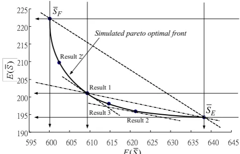
Fig. 5 represents the E-F graph of the simulation system. The relative simulation results shown in Table IV are depicted in this figure as Results 1, 2, 3 and 2’, respectively. The bolder line is the pareto-optimal front of this test system obtained from (16) by the applied PSO, such that w is changing from 0 to 1 for every 0.01 step. There are two pairs of dash lines with different types in Fig. 5 representing the simulation approach of Result 1 and 2 in Table IV. Fig. 5 shows the ability of the proposed approach to automatically and precisely provide a valuable trade-off solution among the pareto-optimal front of the bi-objective problem, a decision that can easily be made according to the preference of the decision maker. Table V represents the generator output of 6-unit system by proposed approach.
TABLEV:OUTPUT OF 6-UNIT SYSTEM BY PROPOSED APPROACH Output
(p.u.)
Bi-objective optimization
Result 1 Result 2 Result 3 Result 2’ P1 0.25508 0.33102 0.29305 0.18031 P2 0.37233 0.41431 0.39292 0.33390 P3 0.53939 0.53927 0.53963 0.53564 P4 0.69852 0.54156 0.62017 0.85571 P5 0.53939 0.53927 0.53963 0.53564 P6 0.42929 0.46856 0.44860 0.39279
190 195 200 205 210 215 220 225
595 600 605 610 615 620 625 630 635 640 645
Result 1
Result 3
Result 2 Result 2'
) (S F F
S
E
S Simulated pareto optimal front
Fig. 5. Simulation results for case 1. 2)Case 2
This case was a real Tai-power system consisting of 40 units [8], [13]. The load demand of the system was 8550MW. To compare with [8] and [13], this case only deals with the generation cost to demonstrate the applied encoding/decoding structure and PSO. Its best solutions, discovered through the evolutionary process are shown in Table VI. All of the constraints previously mentioned were satisfied. The results show that the proposed approach offers better solution quality than those discovered through real value coded PSO and GA methods.
TABLEVI:BEST SOLUTIONS OF TAI-POWER 40-UNIT SYSTEM OVER 50 TRIALS
Output (MW) Proposed Approach PSO method [8] GA method [13] Line Loss 80.58 87.24 89.76 Total Output 8630.58 8637.26 8641.08 Load Supplied 8550.0 8550.0 8551.32 Cost ($/h) 121,430 130,380 135,070
V. CONCLUSION
REFERENCES
[1] T. Niknam, H. D. Mojarrad, and B. Firouzi, “A new optimization algorithm for multi-objective economic/emission dispatch,” International Journal of Electrical Power & Energy Systems, vol. 46, pp. 283-293, March 2013.
[2] P. H. Chen and H. C. Chen, “Power system economic dispatch considering environmental constraints,” Energy Educ Sci Technol Part A, vol. 28 no. 1, PP. 249-260, October 2011.
[3] A. Farag, S. Al-Baiyat, and T. C. Cheng, “Economic load dispatch multiobjective optimization procedures using linear programming techniques,” IEEE Trans. Power Syst., vol. 10 no. 2, pp. 731-738, 1995.
[4] R. Hooshmand and A. H. Mohammadi, “Emission and economic load & reserve dispatch with frequency constraints in competitive power market,” International Review of Electrical Engineering, vol. 3, no. 4, pp. 682-690, August 2008.
[5] M. A. Abido, multiobjective “Evolutionary algorithms for electric power dispatch problem,” IEEE Trans. Evolut. Comput, vol. 10, no. 3, pp. 315-329, 2006.
[6] Y. Lu, J. Zhou, H. Qin, Y. Wang, and Y. Zhang, “Environmental/economic dispatch problem of power system by using an enhanced multi-objective differential evolution algorithm,” Energy Convers. Manage, vol. 52, no. 2, pp. 1175-1183, 2011.
[7] S. Brini, H. Ben Aribia, H. H. Abdallah, and A. Ouali, “Multi objectives optimization of the active/reactive/environmental dispatch of an electrical network,” International Review of Electrical Engineering, vol. 2, no. 3, pp. 301-309, June 2007.
[8] Z. L. Gaing, “Particle swarm optimization to solving the economic dispatch considering the generator constraints,” IEEE Trans. Power Syst, vol. 18, no. 3, pp. 1187-1195, 2003.
[9] C. C. Kuo, “A novel coding scheme for practical economic dispatch by modified particle swarm approach,” IEEE Trans. Power Syst., vol. 23, PP. 1825-1835, 2008.
[10] P. H. Chen and C. C. Kuo, “Economic-emission load dispatch by refined particle swarm optimization and interactive bi-objective programming,” International Review of Electrical Engineering, vol. 6, no. 5, pp. 2584-2595, October 2011.
[11] M. R. Al-Rashidi and M. E. El-Hawary, “Economic dispatch with environmental considerations using particle swarm optimization,” in Proc. Large Engineering Systems Conference on Power Engineering, 2006; pp. 41-46.
[12] D. B. Das and C. Patvardhan, “New multi-objective stochastic search technique for economic load dispatch,” IEE Proc. Part C Gener. Trsns. & Distrib., vol. 145, no. 6, pp. 747-752, 1998.
[13] P. H. Chen and H. C. Chang, “Large-Scale economic dispatch by genetic algorithm,” IEEE Trans. Power Syst., vol. 10, pp. 1919-1926, 1995.
Po-Hung Chen was born on April 21, 1963, in Taipei, Taiwan. He received the B.S. degree from the National Taiwan University of Science and Technology (NTUST), Taipei, the M.S. degree from the National Tsing Hua University, Hsinchu, Taiwan, and the Ph.D. degree from the NTUST, in 1986, 1989, and 1997, respectively, all in electrical engineering. Since 1989, he has been with the St. John’s University, Taipei, where he is currently a professor in the Department of Electrical Engineering. His current research interests include power system planning, partial discharge measurement, and renewable generation techniques.
Hung-Cheng Chen received both the M. S. and Ph.D. degrees in Electrical Engineering from National Taiwan University of Science and Technology in 1989 and 1993, respectively. He is currently an Associate Professor in the Department of Electrical Engineering, National Chin-Yi University of Technology, Taiwan. His research interests include renewable energy systems, micro grid control, and partial discharge diagnosis.
Feng-Jih Wu is with the St. John’s University, Taipei, where he is currently an associate professor in the Department of Electrical Engineering.
Li-Ming Chen is with the St. John’s University, Taipei, where he is currently a lecturer in the Department of Electrical Engineering.