www.the-cryosphere.net/4/21/2010/
© Author(s) 2010. This work is distributed under the Creative Commons Attribution 3.0 License.
The Cryosphere
Geometric changes and mass balance of the Austfonna ice cap,
Svalbard
G. Moholdt, J. O. Hagen, T. Eiken, and T. V. Schuler
Department of Geosciences, University of Oslo, Box 1047 Blindern, 0316 Oslo, Norway Received: 17 September 2009 – Published in The Cryosphere Discuss.: 13 October 2009 Revised: 29 December 2009 – Accepted: 6 January 2010 – Published: 19 January 2010
Abstract. The dynamics and mass balance regime of the
Austfonna ice cap, the largest glacier on Svalbard, deviates significantly from most other glaciers in the region and is not fully understood. We have compared ICESat laser altime-try, airborne laser altimealtime-try, GNSS surface profiles and radio echo-sounding data to estimate elevation change rates for the periods 1983–2007 and 2002–2008. The data sets indicate a pronounced interior thickening of up to 0.5 m y−1, at the same time as the margins are thinning at a rate of 1–3 m y−1. The southern basins are thickening at a higher rate than the northern basins due to a higher accumulation rate. The over-all volume change in the 2002–2008 period is estimated to be −1.3±0.5 km3w.e. y−1 (or −0.16±0.06 m w.e. y−1) where the entire net loss is due to a rapid retreat of the calving fronts. Since most of the marine ice loss occurs below sea level, Austfonna’s current contribution to sea level change is close to zero. The geodetic results are compared to in-situ mass balance measurements which indicate that the 2004– 2008 surface net mass balance has been slightly positive (0.05 m w.e. y−1) though with large annual variations. Sim-ilarities between local net mass balances and local elevation changes indicate that most of the ice cap is slow-moving and not in dynamic equilibrium with the current climate. More knowledge is needed about century-scale dynamic processes in order to predict the future evolution of Austfonna based on climate scenarios.
1 Introduction
Glaciers and ice caps are expected to be significant contrib-utors to sea level rise in the 21st century (e.g. Meier et al.,
Correspondence to: G. Moholdt
(geirmoh@geo.uio.no)
2007). Traditionally, regional and global mass balances have been extrapolated from a series of local mass balance es-timates acquired from annual stake and snow pit measure-ments (e.g. Dyurgerov and Meier, 1997; Dowdeswell et al., 1997; Hagen et al., 2003b). Remote sensing techniques like photogrammetry, altimetry and synthetic aperture radar (SAR) have made it possible to expand mass balance mea-surements to vast and remote areas. Airborne laser altimetry has been widely used to measure elevation changes, e.g. in Alaska (Arendt et al., 2006), Arctic Canada (Abdalati et al., 2004) and Svalbard (Bamber et al., 2005). Glacier changes have also been quantified using spaceborne techniques like the Shuttle Radar Topography Mission (SRTM) (Rignot et al., 2003), the Ice, Cloud and land Elevation Satellite (ICE-Sat) (Nuth et al., 2010) and the Gravity Recovery and Cli-mate Experiment (GRACE) (Luthcke et al., 2008).
The Svalbard archipelago has a total glacier area of ∼36 000 km2 (Hagen et al., 2003a) which is about 7% of the worldwide glacier coverage outside of Greenland and Antarctica (Lemke et al., 2007). Several studies have shown that the mass balance of western Svalbard glaciers has been negative over the last century (e.g. Hagen et al., 2003b; Nuth et al., 2007). Kohler et al. (2007) claim that the glacier thin-ning rates in western Svalbard have been accelerating over the last few decades. The mass balance of eastern Sval-bard glaciers is more uncertain due to a lack of long-term mass balance programs and few repeated geodetic observa-tions. Nuth et al. (2010) compared topographic maps from 1965–1990 with recent ICESat altimetry to find that Sval-bard glaciers have been thinning at an average water equiva-lent (w.e.) rate of 0.36 m w.e. y−1over the last few decades. However, this study did not include Austfonna which at ∼8000 km2is the largest single ice body within the Svalbard archipelago.
Drewry, 1989; Pinglot et al., 2001), but no continuous records of mass balance exist until 2004 when an an-nual mass balance program was initiated. Photogrammetric records are also sparse over Austfonna due to the large ex-tent and featureless topography which make image analysis extremely difficult. Airborne laser altimetry from 1996 and 2002, indicated thickening of up to 0.5 m y−1 in the sum-mit area and thinning towards the margins (Bamber et al., 2004). The authors proposed that this growth was due to in-creased precipitation related to the loss of perennial sea ice cover in the adjacent Barents Sea. A mass build up in the accumulation area was also found by Bevan et al. (2007) who compared surface velocities derived from differential SAR interferometry (DInSAR) with calculated balance ve-locities across the glacier equilibrium line altitude (ELA). They suggested an underlying dynamic component to the changes since 75% of the mass gain was attributed to three basins that are expected to be in the quiescent phase of their surge cycles.
We compare several sources of altimetric observations over Austfonna to estimate elevation change rates for the pe-riods 1983–2007 and 2002–2008. The data sets include air-borne radio echo-sounding (RES) data from 1983 and 2007, GNSS (Global Navigation Satellite System) surface profiles from 2004–2008, airborne laser altimetry from 2002, 2004 and 2007, and ICESat laser altimetry from 2003–2008. We use a combination of repeat track analysis and crossover points to estimate average elevation change rates, and then we combine them in a hypsometric way to derive volume change rates. Finally, the geodetic change rates are compared to in situ mass balance measurements from 2004–2008.
2 Study site
Austfonna is a∼8000 km2large polythermal ice cap located at 80◦N on Nordaustlandet island in the northeast corner of Svalbard (Fig. 1c). The ice cap geometry is characterized by one main ice dome which rises gently up to about 800 m a.s.l. and feeds a number of drainage basins (Fig. 1a). Apart from a few fast flowing units, most of the ice cap is slow-moving with typical velocities less than 10 m y−1 (Dowdeswell et al., 1999; Strozzi et al., 2008). Surge advances have been reported for three of the basins (Fig. 1a), namely Eton-breen (1938), BraasvellEton-breen (1937) and Basin 3 (∼1873) (Lefauconnier and Hagen, 1991). About 30% of the ice cap is grounded below sea level, with ice thicknesses typically ranging from<300 m in the marine southeast to∼500 m in the interior (Dowdeswell et al., 1986). The grounded calving fronts have a total length of 230 km and have been retreat-ing durretreat-ing the last decades. Dowdeswell et al. (2008) used satellite images from between 1973 and 2001 to estimate a mean area loss rate of 11 km2y−1, of which 90% was due to marine retreat. By combining this data with terminus ice thicknesses from 1983 RES and velocities from 1996
DIn-SAR, they were able to estimate a total iceberg calving flux of 2.5±0.5 km3w.e. y−1.
Meteorological conditions at Austfonna are very variable due to its location at the confluence zone between cold and dry polar air masses from the north and more humid and warm air masses from the North Atlantic current to the south. Two automatic weather stations (Fig. 1a) collecting data on Austfonna since 2004 show that the mean daily winter tem-peratures range from about−30◦C to 0◦C. The meteorolog-ical conditions during the summer season are less variable; daily temperatures usually range from 0◦C to 5◦C during the 1–2 months long ablation period. Most of the winter precipitation over the ice cap is originating from the Bar-ents Sea in the southeast, resulting in a pronounced accu-mulation gradient with most snow in the southeast and least snow in the northwest (Schytt, 1964; Pinglot et al., 2001; Taurisano et al., 2007). This pattern is also recognized in the equilibrium line altitude (ELA) which is significantly lower in southeast than in northwest (Pinglot et al., 2001; Schuler et al., 2007). Pinglot et al. (2001) estimated an average net mass balance of 0.5 m w.e. y−1 in the summit area for the period 1986–1998/99 by detecting the depth of the radioac-tive 1986 Chernobyl layer in 19 shallow ice cores (Fig. 1a). Since 2004, in-situ mass balance measurements have been carried out each spring along several transects (Fig. 1a). In addition to point measurements using mass balance stakes and snow pits, the annual snow cover has been mapped using an 800 MHz ground penetrating radar (GPR) supplemented by manual probing to the previous summer surface (Kohler et al., 1997; Taurisano et al., 2007). The annual accumula-tion can vary by a factor of two, but the spatial pattern re-mains more or less similar from year to year. Taurisano et al. (2007) used spatial multiple regression to compile an ac-cumulation index map for the distribution of acac-cumulation. This was further used by Schuler et al. (2007) to model the surface mass balance using a distributed temperature-index approach (Hock, 1999).
3 Data
Fig. 1. (a) Classification of drainage basins into southern, northern and surge type regions. The basins that are known to have surged
are Etonbreen (S1), Braasvellbreen (S2)and Basin 3 (S3). Also shown are the locations of mass balance data used in Fig. 5: 2004–2009 mass balance stakes with average velocities, 2004/08 repeat track GNSS surface profiles, 1998/99 shallow ice cores (Pinglot et al., 2001), and 2004–2009 automatic weather stations. The other plots show estimates of elevation change rates in 2 km clusters for: (b) 2002–2008 crossover points (ICESat, airborne laser and GNSS) and 2004–2008 repeat track GNSS, (c) 2003–2008 repeat track ICESat, and (d) 1983– 2007 RES ice thickness crossover points. The spatial coverage of the different altimetry data sets is plotted in greyscale. The inset (in c) shows the location of Austfonna within the Svalbard archipelago.
National Space Institute at the Technical University of Den-mark (NSI-DTU) in 2004/07 (Forsberg et al., 2002), and by the Alfred Wegner Institute (AWI) in 2005/06. We only use the data sets from 2002, 2004 and 2007 (Table 1 and Fig. 1b), because 1996–2002 elevation differences have already been published (Bamber et al., 2004), and the AWI data sets co-incide largely with simultaneous GNSS ground profiles. The individual airborne laser instruments have slightly different characteristics though all provide a dense sampling (<10 m spacing) of elevation points within a 100–300 m wide ground track. Elevation errors mainly arise from the aircraft GNSS positioning, the inertial navigation system attitude determi-nation, and the laser ranging itself. Krabill et al. (2002) anal-ysed crossover elevation differences and found a root-mean square (RMS) elevation accuracy better than 0.1 m for a sim-ilar instrument setup at the Greenland ice sheet.
The spaceborne Geoscience Laser Altimeter System (GLAS) onboard ICESat is designed to collect high preci-sion surface elevations all over the globe. Since winter 2003,
Table 1. Elevation data sets with years of measurements and estimated precision for single point measurements. Also shown are the methods
of elevation change calculation and the associated accuracy of single point elevation changes. ICESat data has a dh accuracy of 0.5 m for crossover points and 1 m for repeat track points. The accuracy of RES ice thickness changes is not assessed due to potential systematic errors related to the RES signal processing in 1983 and 2007.
Data source Year hprecision dh accuracy Method
ATM laser 2002 <0.10 m 0.5 m Crossovers DTU laser 2004, 2007 <0.10 m 0.5 m Crossovers
GNSS 2004–2008 <0.10 m 0.5 m Crossovers or repeat track ICESat 2003–2008 <0.10 m 0.5 or 1 m Crossovers or repeat track SRPI RES 1983 ∼22 m NA Ice thickness crossovers DTU RES 2007 ∼8 m NA Ice thickness crossovers
to the elevations to account for the delay of the pulse cen-tre in saturated returns (Fricker et al., 2005). We also con-verted ICESat data from the TOPEX/Poseidon ellipsoid to the WGS84 ellipsoid to ensure compatibility with GNSS and airborne altimetry data which refer to WGS84.
The altimetry data set with the best spatial coverage across Austfonna is from an airborne radio-echo sounding (RES) campaign carried out by the Scott Polar Research Institute (SPRI) and the Norwegian Polar Institute (NPI) in spring 1983 (Dowdeswell et al., 1986). Measurements were per-formed along a 5–10 km grid using a 60 MHz RES instru-ment (Fig. 1d) that registered both surface and bedrock re-turns. The positioning of the aircraft relied on a ranging system from the airplane to four ground-based transponders of which the position was accurately determined by satel-lite geoceivers. A more precise airplane altitude was deter-mined from a pressure altimeter which was frequently cali-brated over sea level in order to minimize errors from tem-poral pressure variations. However, such a calibration does not account for potential biases arising from local pressure anomalies across the ice cap. Pressure measurements in spring 2008 indicated that the air pressure at the center of the ice cap can deviate significantly (∼3 hPa) from the pre-dicted pressure based on simultaneous measurements at the coast. The pressure at the center was typically higher than ex-pected during periods of calm and clear weather. If such con-ditions were ambient during the 1983 RES survey, this would have resulted in a systematic elevation underestimation of up to 20–30 m in the ice cap interior. To avoid inaccuracies in our elevation change estimates caused by this potential bias, we chose to use RES ice thickness data instead. Ice thick-ness was estimated from the time difference between tracked surface and bedrock echoes multiplied by the signal velocity and should thus be independent of air pressure. A few pro-files of 60 MHz RES were also obtained in spring 2007 by NSI-DTU (Fig. 1d) simultaneously with the laser profiling described earlier. The aircraft position was precisely deter-mined by three onboard GNSS receivers, and the RES ice thickness processing was done in a semi-automatic way
us-ing a surface and bottom detection software (Kristensen et al., 2008).
In order to convert volume changes into mass changes, in-formation about the temporal evolution of the firn pack is needed. Several firn thickness and density profiles were ob-tained from shallow ice cores in spring 1998 and 1999 (Pin-glot et al., 2001). A few∼15 m shallow ice cores were also drilled in 2006 and 2007. Since 2004, the annual snow pack and glacier facies have been investigated by snow pits, prob-ing and GPR profilprob-ing (Taurisano et al., 2007; Dunse et al., 2009). A neutron probe was used in spring 2007 to obtain four high resolution firn density profiles in connection with CryoSat-2 calibration work (Brandt et al., 2008). The bulk firn densities are typically ranging from 400 to 600 kg m−3 with some ice layers of higher density and a general increase of density with depth.
The geodetic change rates were also compared to point mass balance measurements acquired in annual field cam-paigns from 2004 to 2008. Stake and snow pit measurements have been carried out in late April/early May along several transects (Fig. 1a). Stake heights were measured down to the snow surface and down to last year’s summer surface, and precise stake positions were determined by static∼5 min dif-ferential GNSS surveys. The bulk density of the winter snow pack was measured annually in snow pits at stake locations, while the density of the summer snow pack was sampled in a few deeper snow/firn pits. The only stake transect that has been repeated each year is that from Etonbreen to the summit (Fig. 1a).
4 Methods
(dh/dt) for all possible time intervals spanning three years or more within the 2002–2008 period. In order to avoid sea-sonal elevation biases in our analysis, we only compared data between similar seasons, e.g. winter to winter and fall to fall. Using average dh/dt rates from various elevation data sets and time spans allows for a robust estimation of the overall volume change and geometric change trend over the 2002– 2008 period.
Elevation change rates were calculated at crossover points between two profiles (within and between GNSS, airborne laser and ICESat) and along repeated tracks (within GNSS or ICESat). Elevations at crossover points were determined by linear interpolation of the measurements between the two closest footprints within 200 m distance in each profile (Fig. 2a). The elevation differences (dh) at each crossover point were divided by the number of years (dt≥3 y) between the two surveys to obtain elevation change rates (dh/dt). Re-peat track profiles in the GNSS and ICESat data sets were compared separately. Surface GNSS profiles are generally repeated within a stripe of 10–15 m width, and individual tracks cross each other frequently and randomly. Hence, we compared each GNSS point in one profile to the closest point in another profile within a radius of 5 m. This ensures a suf-ficiently dense sampling of dh/dt points. Furthermore, the vertical error due to cross-track slope is kept minimal since a typical Austfonna surface slope of 1◦over 5 m would intro-duce a relative elevation bias of less than 0.10 m.
It is difficult to compare repeat track ICESat profiles due to the relatively large cross-track separation distance between repeating profiles. The average cross-track separation of 90 m at Austfonna with a 1◦ slope would introduce a rela-tive elevation bias of 1.6 m. We used a new digital elevation model (DEM) of 25 m horizontal resolution to correct for ele-vation differences caused by the cross-track slope. The DEM was constructed from DInSAR with ground control points from ICESat altimetry. The local slopes of the DEM should not be affected by the ICESat points since they are only used to reconstruct the overall geometry of the SAR acquisitions (i.e. baseline refinement). For each pair of ICESat repeat tracks, the oldest profile was chosen as the reference profile. The second profile was projected onto the reference profile using the cross-track elevation differences in the DEM. El-evation change was then calculated at each DEM-projected point along the reference profiles by linearly interpolating neighbouring footprints along the reference profiles to the re-spective point locations (Fig. 2b). Repeat pass dh/dt points derived with a cross-track separation larger than 200 m or a DEM correction larger than 5 m were ignored.
The calculated dh/dt points from crossover and repeat track analysis were unevenly distributed in space and often represented change rates from different time spans and meth-ods. In order to obtain a robust estimate of the overall eleva-tion change trend over the 2002–2008 period, we averaged all
dh/dt points within 2 km clusters for the data sets in Fig. 1b
(crossover points and GNSS repeat track data) and Fig. 1c
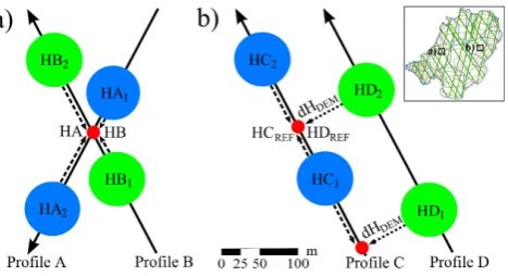
Fig. 2. The inset map shows all ICESat profiles on Austfonna and
an example of two locations where elevation change can be esti-mated: (a) a crossover point where two altimetry profiles (A and B) intersect each other. Linear interpolation between the two clos-est footprints was used to determine the crossover point elevation for each profile (HA and HB). The difference between the two el-evations (dh=HB−HA) is the estimated elevation change at the crossover point. (b) Repeat track ICESat observations were com-pared stepwise: (1) choose one profile as the reference profile (C). (2) Project each footprint from the other profile (D) perpendicu-larly to the reference profile (C) by means of the extracted ele-vation difference between the two locations in a DEM (HDREF= HD2+dHDEM). (3) Estimate the elevation of the reference profile (HCREF)at each DEM-projected point using linear interpolation between the two closest footprints (HC1and HC2). (4) Calculate the elevation difference for each point pair along the reference pro-file to derive estimates of elevation change (dh=HDREF−HCREF).
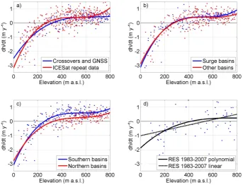
(ICESat repeat track data). The clustered dh/dt points were then plotted as a function of elevation (Fig. 3a), and higher order polynomial functions were fitted to the data (e.g. K¨a¨ab, 2008). Ther2coefficient of determination and the RMS er-ror of the polynomial fits were typically stabilizing (r2∼0.7 and RMS∼0.4 m) after adding a third order coefficient. Thus, third order polynomial fits were used to parameterize all ele-vation change – eleele-vation relationships (Fig. 3).
Fig. 3. (a) Elevation change rates (2 km clusters) versus elevation for the two data sets in Fig. 1b (2002–2008 crossover points and 2004–2008
repeat track GNSS) and Fig. 1c (2003–2008 repeat track ICESat). (b) 2002–2008 elevation change rates for surge type basins versus other basins. (c) 2002–2008 elevation change rates for southern basins versus northern basins. The locations of the different basins are shown in Fig. 1a. The two data sets in (a) were mixed and clustered (2 km) before forming the data sets of (b) and (c). (d) shows 1983–2007 elevation change rates for RES ice thickness crossover points (Fig. 1c). Solid lines show third order polynomial fits to the dh/dt points (a–d), while the dashed line in (d) is a linear fit.
Fig. 4. Hypsometries for the southern basins, northern basins (Fig. 1a) and the Eton-/Winsnesbreen basin (Fig. 6). Glacier ar-eas were extracted for each meter of elevation from a new DIn-SAR/ICESat DEM which the polynomial fits of elevation change and mass balance were integrated over to obtain volume change rates. Note the relatively large glacier areas at low elevations in the southern basins.
It is expected that the geometric changes vary regionally and from basin to basin due to the accumulation gradient across Austfonna and the surge-type characteristics of some drainage basins. Comparative dh/dt calculations were done for the southern basins versus the northern basins (Figs. 1a and 3c) and for surge-type basins versus basins without any reported surge history (Figs. 1a and 3b). Here, the crossover points and GNSS repeat track data (Fig. 1b) were mixed and clustered (2 km) with the ICESat repeat track data (Fig. 1c) in order to obtain a better spatial distribution of dh/dt points within the selected regions. The sum of the regional dV/dt rates was then used to estimate the total dV/dt and the glacier-wide dh/dt.
2008 period. Dunse et al. (2009) derived from GPR profil-ing that the firn line elevation increased slightly from 2003 to 2004 (<50 m) and then lowered over the next two years from∼650 m to∼550 m elevation in the northwest and from ∼600 m to 4–500 m in the southeast. Based on this, we cal-culatedbminusing the density of ice (ρice=900 kg m−3) for all changes below the firn line (super-imposed ice area and abla-tion area) and the average density of firn (ρfirn=500 kg m−3) for all changes above the firn line. Average firn line eleva-tions of 600 m and 500 m were used for the northern and the southern basins respectively. The real mass balance is ex-pected to lie somewhere between these two extreme cases of firn density conversion. We used the average ofbminand bmaxas the final estimate of water equivalent mass balance (b).
The effect of glacier retreat and advance on area-averaged
dh/dt rates is usually accounted for by dividing the total
vol-ume change by the average glacier area of the measurement period (e.g. Arendt et al., 2002). However, most of Aust-fonna is terminating into the sea, and ice volume changes below sea level can not be measured by laser altimetry or GNSS. Elevation change measurements in the proximity of the 20–40 m high calving fronts can also vary by tens of me-ters over short distances due to terminus fluctuations. There-fore, we excluded all observations below 25 m a.s.l. in the polynomial fitting. Instead we applied marine loss rates from Dowdeswell et al. (2008) to consider terminus changes in the total mass balance.
The RES ice thickness data sets from 1983 and 2007 were compared by calculating the difference in ice thickness at 75 crossover points and dividing by the 24 years time span (Fig. 1d). A linear regression curve (r2=0.20) and a third or-der polynomial curve (r2=0.23) were fitted to the ice thick-ness change points (dh/dt) in order to reveal possible eleva-tion change trends over the 1983–2007 period (Fig. 3d). Vol-ume change and mass balance were not calculated from the RES measurements due to the high noise level and the possi-bility of systematic errors.
Surface net mass balance was estimated for each stake from the difference in stake height down to the previous sum-mer surface between two consecutive years. The density of ice (ρice=900 kg m−3) was used to convert stake height changes into mass changes in the ablation or super-imposed ice areas, while the average density of firn (ρfirn=500 kg m−3) was used for all stakes in the firn areas. The estimate of ρfirn was based on density measurements in the uppermost firn layer in snow/firn pits, shallow ice cores (Pinglot et al., 2001) and neutron probe profiles (Brandt et al., 2008; Dunse et al., 2009). The annual net mass balances were averaged over the 2004–2008 period. Only stake measurements that covered the entire time span were used in the analysis. We parameterized the mass balance – elevation relationship by fitting polynomial functions to the data (Fig. 5), separately for the southern and northern basins. The RMS andr2of the fits stabilized after adding a second order coefficient. The
second order polynomial functions were then integrated over the DInSAR/ICESat DEM (Fig. 4) in order to obtain esti-mates of the volume change rates excluding calving. Since all stake data were referenced to previous summer surfaces, the 2004–2009 spring measurements yielded mass balance rates for the period between fall 2003 and fall 2008 (5 mass balance years).
In order to investigate the relation between local surface mass balance and elevation change, we extracted two repeat track GNSS surface profiles from 2004 and 2008 along the main mass balance transects (Fig. 1a). Along-track elevation differences were calculated and smoothed using a running mean filter over 2 km distances. The elevation changes were then converted to water equivalent rates using the density of ice (ρice=900 kg m−3) and plotted as a function of elevation along with the surface mass balance curves in Fig. 5.
Annual and seasonal mass balances were calculated for the Eton-/Winsnesbreen basin which is the only mass bal-ance profile that has been measured each year since 2004. Winter mass balances at stakes were derived from the snow depth in the subsequent spring considering the bulk density measured in snow pits. Summer mass balances were ob-tained by subtracting the winter balances from the net bal-ances. Second order polynomial functions were used to ex-trapolate the point observations to all elevations of the Eton-/Winsnesbreen part of the DEM (Fig. 4) and to calculate vol-ume changes. Area-averaged specific winter, summer and net mass balances were calculated for each year from 2004 to 2008 by dividing the volume changes by the basin area (Fig. 6).
5 Error analysis
The uncertainty of an area-averaged elevation change rate (ε
dh/dt) is equal to the standard error of the polynomial fit
assuming that elevation change points are randomly spatially distributed, have no spatial autocorrelation and no systematic elevation errors:
εdh/dt=√σfit
f (1)
Fig. 5. The continuous lines are second order polynomials fitted to
averaged point observations of annual net mass balances between fall 2003 and fall 2008 in the southern and northern basins (Fig. 1a). The area-averaged surface mass balance is 0.09 m w.e. y−1 for the southern basins and−0.01 m w.e. y−1for the northern basins, giving an overall specific mass balance of 0.05 m w.e. y−1 (or 0.38 km3w.e. y−1). The average equilibrium line altitude (ELA) is 300 m in the south and 450 m in the north which corresponds to an overall accumulation-area ratio (AAR) of 60 %. The 1986–1998/99 average net mass balances from shallow ice cores are included for comparison (Pinglot et al., 2001). The dashed lines show the av-erage water equivalent elevation change rates between spring 2004 and spring 2008 along two repeat track GNSS profiles that follow the mass balance transects (Fig. 1a).
was found between two overlapping GNSS and laser profiles obtained within a few days time in 2007. In the lack of more overlapping observations, we assume that systematic eleva-tion errors are small and mainly random due to the variety of measurement techniques and time spans involved in the analysis. Thus, the three assumptions of the standard error equation are fulfilled.
The error budget of a geodeticdh/dt calculated from a limited sample of elevation change points can be divided into an observation error and an extrapolation error (e.g. Arendt et al., 2002; Nuth et al., 2010). The error of crossover dh/dt points can be quantified by analysing crossovers within short time spans where no significant elevation change is expected. Within individual ICESat observation periods (dt<30 d), the interquartile range (IQR) of 113 crossover points at Aust-fonna was 0.46 m. Similar findings have been reported for comparable slopes in Greenland and Antarctica (Brenner et al., 2007). The airborne laser profiles have much fewer crossover points, but the precision should lie well within that of ICESat. For simplicity, we set an error estimate (εcross) of 0.5 m for all crossover points. Errors in repeat track compar-isons are mainly due to track divergence. Hagen et al. (2005) found that the precision of GNSS profiles that were measured twice during the same field campaign was better than 0.3 m
Fig. 6. Annual and seasonal surface mass balances for the
Eton-/Winsnesbreen basin based on annual spring measurements. The inset map shows the basin location and the mass balance stakes that were used in the calculations. Annual ELAs are shown at the bot-tom. Note the rise in annual net mass balance and ELA from 2004 to 2008. The overall net mass balance of the basin is 0.02 m w.e. y−1 and the overall ELA is 460 m (66% AAR) over the 5 years period.
even when the tracks were up to 90 m apart. However, we also accept a generous error estimate (εGNSS) of 0.5 m for the GNSS repeat track data. The main error component in the re-peat track ICESat analysis is the cross-track DEM correction. This DEM error can be estimated by comparing elevation differences between pairs of altimetric points (e.g. the eleva-tion difference between two neighbour ICESat points in the same ground track) with the elevation differences between the corresponding point pair locations in the DEM. The rel-ative error of the DEM ranges from ∼0.4 m (IQR) over a 50 m distance to∼1.4 m over a 170 m distance. The addi-tional error due to along-track interpolation should be less than the crossover point error at 0.5 m. Based on an average cross-track separation of 90 m between repeating profiles, we accept 1 m for the repeat track ICESat point error (εICESat). Assuming that all elevation change points within each 2 km cluster are fully correlated, the cluster error (εclust) equals the mean of the individual point errors within that cluster:
εclust= 1 n
n
X
i=1 εPT
dt
i
(2)
When we assume that there is no spatial autocorrelation between the clusters, it implies that the effect of cluster er-rors on the overall elevation change rate is reduced with an increasing number of clusters (N). The cluster errors (εclust) can thus be combined into an overall observation error (εOBS) related to the uncertainty of the measurements:
εOBS= v u u t1/
N
X
i=1 1 εclust2
i
(3)
The area-averaged elevation errorεdh/dtis a combined result of the observation error (εOBS) and the spatial extrapolation errorεEXT. SinceεOBSandεEXTare independent, they will combine as root-sum-squares (RSS) to formεdh/dt. Thus, the unknown extrapolation errorεEXTcan be estimated from: εEXT=
q
εdh/dt2−ε
OBS2 (4)
The error introduced when converting elevation change to water equivalent mass change is more difficult to quantify due to the temporal variation in firn thickness and density. In-stead, we provide a minimum (bmin) and a maximum (bmax) estimate of the mass balance. The range between these two extreme values can be used to estimate a density conversion error:
ερ=
1
2(bmax−bmin) (5)
We also have to account for ice losses due to calving front re-treat in the total estimate of Austfonna’s mass balance. This adds an additional error (εRETR=ERETR/A) in the mass bal-ance that follows from the volumetric retreat error estimate (ERETR) of Dowdeswell et al. (2008) and the glacier area (A). All the described error components can finally be combined as RSS to form the total mass balance error estimate: εb=
q
εOBS2+εEXT2+ερ2+εRETR2 (6) Volumetric errors (E)are easily obtained by multiplying the specific errors (ε) with the glacier area. In order to see the in-fluence of the errors at different elevations, the computations above can be done separately for a number of elevation bins. Figure 7 shows the different error components as a function of elevation for 50 m elevation bins. The RSS of the volumet-ric bin errors will be equal to the overall volumetvolumet-ric errors if the elevation change points are randomly distributed over the ice cap.
The ice thickness comparison between 1983 and 2007 (Fig. 3d) is too coarse for a thorough error analysis. The precision of the 1983 ice thickness data is 22 m based on the IQR of 167 crossover points, while the 2007 ice thick-ness data have a precision of 8 m (IQR) and an accu-racy of∼1 m (mean error) as compared to overlapping low-frequency (20 MHz GPR) surface profiles from 2008. Al-though the random errors are fairly well known, we can not
Fig. 7. Area-averaged elevation errors for 50 m elevation bins. There are three error components that vary with elevation; a spa-tial extrapolation error (εEXT), an observation error (εOBS), and a density conversion error (ερ). The two first ones (εEXTandεOBS) are random errors that combine as a RSS in the overall error, while the last one (ερ) is a systematic error that must be summed up
in the error budget. The overall area-averaged error components are 0.02 m w.e. y−1forεEXT, 0.01 m w.e. y−1forεOBS, and 0.03 m w.e. y−1forερ, resulting in a total RSS error of 0.04 m w.e. y−1
in the area-averaged geodetic mass balance. An additional error component from the marine retreat loss (εRETR) must be consid-ered when assessing the total mass balance including calving front retreat (Table 2).
exclude the possibility of systematic errors attributed to dif-ferences in the RES signal processing between the 1983 and 2007 campaigns. The RES data sets are thus better suitable for interpretation of geometric change than for calculation of volume change.
6 Results and discussion
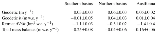
Table 2. Geodetic estimates of area-averaged elevation change rates (dh/dt) and mass balances (b) between 2002 and 2008 for the south-ern basins, northsouth-ern basins and the entire Austfonna. The total mass balance is estimated by adding the calving front retreat loss dV/dt (Dowdeswell et al., 2008) to the geodetic dV/dt and dividing by the corresponding glacier area. One standard deviation error estimates are provided for each change rate.
Southern basins Northern basins Austfonna
Geodetic (m y−1) 0.03±0.03 0.06±0.03 0.05±0.02 Geodeticb(m w.e. y−1) −0.01±0.05 0.04±0.03 0.01±0.04 Retreat dV/dt (km3w.e. y−1) −1.1±0.03 −0.3±0.02 −1.4±0.4 Total mass balance (m w.e. y−1) −0.25±0.08 −0.04±0.06 −0.16±0.06
Mass build up in the accumulation area combined with deficits in the ablation area is typical for glaciers in a qui-escent phase of their surge cycle. Bevan et al. (2007) found that the accumulation areas of surge-type basins at Aust-fonna were thickening at a higher rate than most other basins. Our elevation change curves for known surge-type basins versus other basins (Fig. 3b) do not indicate a clear differ-ence in geometric change between these two glacier types at Austfonna. However, the area-averaged elevation change is slightly more negative for the three surge-type basins due to their relatively large areas at low elevations, the aftermath of previous surges. Potential differences in geometric change between individual basins are probably of smaller magni-tudes than the overall change pattern which is seen across all basins. The general trend towards surface steepening sug-gests that other basins might also be capable of surging in the future. Lefauconnier and Hagen (1991) suggest that up to 90% of Svalbard’s glaciers are surge-type, although most of them lack historic records of surges.
The southern basins are generally thickening at a faster rate than the northern basins (Fig. 3c). This is in agreement with the southeast to northwest accumulation gradient across Austfonna (Taurisano et al., 2007). The elevation change curves of the southern and northern basins are crossing the zero change line at elevations of 260 m and 330 m, respec-tively. This is a smaller south to north gradient than what is seen in ELA estimates from shallow ice cores (Pinglot et al., 2001) and from mass balance stakes (Fig. 5). The aver-age ELA for the 2004–2008 period is 300 m for the southern basins and 450 m for the northern basins which agrees well with the long-term lower boundary of the super-imposed ice area mapped by Dunse et al. (2009). The southern and north-ern ELAs correspond to an average accumulation-area ratio (AAR) of 60%.
Elevation change curves can not be directly compared with surface mass balance curves due to glacier dynamics. How-ever, if a glacier is stagnant or moves at very low veloci-ties, the two curves will approach each other as was observed for Kongsvegen, a surge-type glacier in western Spitsbergen (Melvold and Hagen, 1998). Velocity fields from DInSAR (Bevan et al., 2007; Strozzi et al., 2008) and annual GNSS
measurements of mass balance stake movements (Fig. 1a) show that, apart from a few fast flowing units (Dowdeswell et al., 1999), most of Austfonna is stagnant at velocities <10 m y−1. This is probably the main reason why the inte-rior of Austfonna appears to be in a steady phase of growth. Bevan et al. (2007) found that the overall ice flux across the ELA in winter 1994/96 was only half of the mean 1986–1999 annual net mass balance above the ELA (Pinglot et al., 2001). The two elevation change curves in Fig. 5 follow the general trend of the corresponding surface mass balance curves, im-plying that the ice flow (Fig. 1a) is far too slow to balance out the current accumulation rate. Hence, the main pattern of elevation change at Austfonna is dominated by the surface mass balance with the ice submergence/emergence playing a secondary role.
the northwest are shown in Fig. 6. From 2004 to 2008, the annual net mass balance increased for each year from a very negative 2004 (−0.51 m w.e. y−1) to a very positive 2008 (0.49 m w.e. y−1). This remarkable trend is a combined ef-fect of increased winter accumulation and reduced summer ablation during the 5 years of observation. The concurrent lowering of the annual ELA at Eton-/Winsnesbreen was from 660 m (18% AAR) in 2004 to 120 m (97% AAR) in 2008. This lowering of the ELA coincides with the 2003–2006 firn area expansion mapped by Dunse et al. (2009), and must have caused an overall upbuilding of firn during the 2002– 2008 geodetic observation period. Still, using the density of firn (ρfirn=500 kg m−3) to convert elevation changes to mass changes in the firn area will probably cause an underestima-tion of the mass balance due to firn densificaunderestima-tion and inter-nal refreezing over the 6 years time span (e.g. Brandt et al., 2008). In order to provide one total number for the geodetic mass balanceb (excluding calving front retreat) during the 2002–2008 period (Table 2), we therefore took the average of the lower estimatebmin(ρfirn=500 kg m−3) and the upper estimatebmax(ρfirn=ρice).
For tidewater glaciers, the iceberg calving flux must be included in the total mass balance budget. Dowdeswell et al. (2008) estimated a total iceberg calv-ing flux of 2.5±0.5 km3w.e. y−1 for Austfonna, where ∼1.1 km3w.e. y−1 was due to the ice flux at the calving fronts and ∼1.4 km3w.e. y−1 was due to calving front retreat. Our geodetic volume change rates account for ice flux calving since the elevation change curves are integrated over the entire glacier area. Marine retreat loss on the other hand is not accounted for since all geodetic measurements below 25 m elevation were excluded from the analysis due to the discrete nature of elevation changes along a retreating calving front and the inability of laser altimeters to measure ice thickness changes below sea level. With almost no geodetic volume change above the calving fronts between 2002 and 2008, the best estimate of Austfonna’s total mass balance becomes almost similar to the proposed marine retreat loss, i.e. −1.3 km3w.e. y−1 (or −0.16 m w.e. y−1). The stake measurements on the other hand yield a total mass balance of −2.1 km3w.e. y−1 (or −0.26 m w.e. y−1) when the total iceberg calving flux (−2.5 km3w.e. y−1) is subtracted from the surface mass balance estimate (0.38 km3w.e. y−1). Before applying calving flux data from Dowdeswell et al. (2008), we have to assume that the marine retreat rates and the velocity fields of the ice cap have not changed significantly between the 1990s and the 2002–2008 period. Annual static GNSS surveys of mass balance stakes between 2004 and 2008 yield average surface velocities of 0.5–13 m y−1 (Fig. 1a) with little temporal variation. And repeat pass ICESat observations across the calving fronts do not indicate any substantial changes in the retreat rates. However, we can not exclude the possibility of a changed calving flux since we lack recent data on terminus ice thick-ness and velocity. The 0.9 km3w.e. y−1difference between
the total mass balance of the geodetic method and the in-situ method indicate that the ice flux calving rate is currently lower than what Dowdeswell et al. (2008) estimated. The discrepancy can also be related to the extrapolation of point measurements to the entire glacier area, or to the slightly different time spans involved, or to the uncertainty of the density conversion factors.
The westerly location of most mass balance stakes could lead to a bias in the overall in-situ estimates towards lower surface mass balances due to less winter accumulation and a relatively higher firn line which exposes more ice to melt-ing at a low albedo durmelt-ing the summer. Also, the surface mass balance at stakes will be underestimated if meltwater or rain percolate through the last summer surface and refreeze in lower firn layers (Paterson, 1994). Brandt et al. (2008) found ice layers in the firn with thicknesses ranging from a few millimeters to more than 0.5 m, indicating substan-tial internal refreezing. Shallow ice core samples from the summit areas approach the density of ice already at 3–6 m depths, with no apparent change of firn thicknesses between 1999 (Pinglot et al., 2001) and 2007 (Brandt et al., 2008). Analysis of a deep ice core from 1987 indicated that 60– 80% of the uppermost 50 m of ice was formed through re-freezing (Zagorodnov and Arkhipov, 1990). Zagorodnov et al. (1990) also noted the presence of sub-surface water pock-ets that form in depressions during years of warm summers when the amount of meltwater exceeds the amount which can refreeze. Surface undulations at a scale of a few kilometers, which are commonly seen on Austfonna, are probably pre-venting the efficiency of meltwater drainage in the firn area. If we assume that all meltwater in the firn area is retained within the firn pack (as refrozen ice or water pockets) and that there is no significant summer accumulation, then the net mass balance at stakes in the firn area will be equal to the winter mass balance. Applied to the stake measurements at Austfonna, this would raise the specific surface mass balance from 0.05 m w.e. y−1 to 0.12 m w.e. y−1. The most realistic surface mass balance will probably lie somewhere between these two extreme cases.
2008 (Fig. 5) as well as between the elevation changes during 1996–2002 (Bamber et al., 2004) and 2002–2008 (Fig. 1) in-dicates that the most recent mass balance conditions are also representative for the last few decades.
Austfonna’s present contribution to sea level change is dif-ficult to quantify due to the uncertain distinction between marine ice losses above and below sea level. If we assume an average ice thickness of 120 m at the calving fronts (de-rived from 1983 RES data) and an average ice cliff height of 30 m above sea level (derived from ICESat altimetry), then the contribution from terminus retreat or advance to sea level change will be ∼17% of the water equivalent ice volume change at the terminus. Thus, Austfonna’s 1.4 km3w.e. y−1 terminus retreat loss will only displace 0.2 km3w.e. y−1 of seawater which is almost balanced by the 0.1 km3w.e. y−1 volume gain above the calving fronts. Austfonna’s negli-gible contribution to sea level rise is in sharp contrast to the rest of Svalbard’s glaciers which have contributed with 9.5±1 km3w.e. y−1 over the last few decades (Nuth et al., 2010).
7 Conclusions and outlook
Austfonna has experienced high elevation thickening, low el-evation thinning and calving front retreat between 2002 and 2008. This geometric change pattern has also been observed recently for several glacier basins in Alaska (Arendt et al., 2008), Greenland (Wouters et al., 2008) and the Antarctic Peninsula (Pritchard et al., 2009). The 2002–2008 results at Austfonna correspond well to the elevation changes de-rived from 1996–2002 airborne laser altimetry (Bamber et al., 2004). Here, we show that the elevation changes are mainly driven by the surface mass balance with the response of surface thickening at high elevations and thinning at low elevations. This is a typical pattern for surge-type glaciers in their quiescent phase of a surge cycle (e.g. Hagen et al., 2005). The interior thickening rate of up to 0.5 m y−1 is higher than what is seen on quiescent phase surge-type glaciers in Spitsbergen over the last few decades (Nuth et al., 2010). The general trend of surface steepening at Austfonna may ultimately lead to surge activity in some of the drainage basins.
The mean mass balance of Austfonna in the 2002– 2008 period is estimated to be −1.3±0.5 km3w.e. y−1 (or −0.16±0.06 m w.e.) when taking into account the marine retreat loss of 1.4±0.4 km3w.e. y−1 from Dowdeswell et al. (2008). It remains uncertain how representative these numbers are for the longer term mass balance of Austfonna. However, shallow ice cores and in-situ mass balance mea-surements do not indicate any significant changes in the mean surface mass balance in the summit area since the 1986–1998/99 period (Pinglot et al., 2001). The 2002–2008 elevation change pattern is also recognized in the 1983–2007 RES ice thickness data, although the accuracy of the RES
data is too low for mass balance calculations. Since there is a lack of high quality geodetic data prior to 1996, further questions on the decadal evolution of the mass balance of the ice cap need to be addressed by means of other methods like e.g. mass balance models utilizing meteorological reanalysis data.
This study underlines that Austfonna in many ways needs to be treated separately from most other glaciers and ice caps in Svalbard when assessing the overall mass budget of the archipelago. While the surface mass balance seems to be close to zero at present, the rapid retreat of the extensive calv-ing fronts is still causcalv-ing a significantly negative total mass balance. The widespread geometric changes imply that Aust-fonna is not in dynamic balance with its current climate. Ge-ometric adjustments of drainage basins through glacier accel-eration or surge activity are likely to occur on a century time scale. Such potential mass redistributions will also largely influence the mass balance regime of the ice cap, i.e. a more negative mass balance after a surge due to the expanded area at low elevations. Austfonna might therefore be out of phase with the surface mass balance regimes of many other glaciers and ice caps on Svalbard due to differences in their past dy-namics. Numerical modelling of Austfonna’s dynamics and mass balance will be a key to gain more insight into the im-portance of these processes in the longer term mass balance evolution of the ice cap.
Acknowledgements. The fieldwork at Austfonna is a joint project between the University of Oslo and the Norwegian Polar In-stitute (NPI). Funding was mainly provided from the CryoSat calibration and validation experiment (CryoVEX) coordinated by the European Space Agency, the International Polar Year project GLACIODYN; the dynamic response of Arctic glaciers to global warming, and the ice2sea project, funded by the European Commission’s 7th Framework Programme through grant number 226375. G. Moholdt was also supported through the Arkisstipend grant from the Svalbard Science Forum (SSF). The authors are thankful to all participants in the annual field campaigns, and to the contributors of high quality altimetric data, namely J. Dowdeswell and T. Benham (1983 RES data), J. Bamber (2002 ATM LIDAR data), NSI-DTU (2004/07 LIDAR and 2007 RES data) and the National Snow and Ice Data Center (ICESat data). Furthermore, we acknowledge C. Nuth, T. Dunse, I. Koch, M. Pelto, L. Copland and an anonymous reviewer for useful comments and contributions to the paper manuscript.
Edited by: I. M. Howat
References
Abdalati, W., Krabill, W., Frederick, E., Manizade, S., Martin, C., Sonntag, J., Swift, R., Thomas, R., Yungel, J., and Ko-erner, R.: Elevation changes of ice caps in the Canadian Arc-tic Archipelago, J. Geophys. Res.-Earth Surface, 109, F04007, doi:10.1029/2003JF000045, 2004.
Altimeter System (GLAS) on the ICESat mission: On-orbit measurement performance, Geophys. Res. Lett., 32, L21S02, doi:10.1029/2005GL024028, 2005.
Arendt, A. A., Echelmeyer, K. A., Harrison, W. D., Lingle, C. S., and Valentine, V. B.: Rapid wastage of Alaska glaciers and their contribution to rising sea level, Science, 297, 382–386, doi:10.1126/science.1072497, 2002.
Arendt, A., Echelmeyer, K., Harrison, W., Lingle, C., Zirnheld, S., Valentine, V., Ritchie, B., and Druckenmiller, M.: Updated estimates of glacier volume changes in the western Chugach Mountains, Alaska, and a comparison of regional extrapola-tion methods, J. Geophys. Res.-Earth Surface, 111, F03019, doi:10.1029/2005JF000436, 2006.
Arendt, A., Luthcke, S. B., Larsen, C. F., Abdalati, W., Krabill, W., and Beedle, M. J.: Validation of high-resolution GRACE mas-con estimates of glacier mass changes in the St Elias Mountains, Alaska, USA, using aircraft laser altimetry, J. Glaciol., 54, 778– 787, 2008.
Bader, H.: Sorge’s Law of densification of snow on high polar glaciers, J. Glaciol., 2, 319–323, 1954.
Bamber, J., Krabill, W., Raper, V., and Dowdeswell, J.: Anomalous recent growth of part of a large Arctic ice cap: Austfonna, Svalbard, Geophys. Res. Lett., 31, L12402, doi:10.1029/2004GL019667, 2004.
Bamber, J. L., Krabill, W., Raper, V., Dowdeswell, J. A., and Oerle-mans, J.: Elevation changes measured on Svalbard glaciers and ice caps from airborne laser data, Ann. Glaciol., 42, 202–208, 2005.
Bevan, S., Luckman, A., Murray, T., Sykes, H., and Kohler, J.: Positive mass balance during the late 20th century on Aust-fonna, Svalbard, revealed using satellite radar interferometry, Ann. Glaciol., 46, 117–122, 2007.
Blaszczyk, M., Jania, J. A., and Hagen, J. O.: Tidewater glaciers of Svalbard: Recent changes and estimates of calving fluxes, Pol. Polar Res., 30, 85–142, 2009.
Brandt, O., Hawley, R. L., Kohler, J., Hagen, J. O., Morris, E. M., Dunse, T., Scott, J. B. T., and Eiken, T.: Comparison of airborne radar altimeter and ground-based Ku-band radar measurements on the ice cap Austfonna, Svalbard, The Cryosphere Discuss., 2, 777–810, 2008,
http://www.the-cryosphere.net/2/777/2008/.
Brenner, A. C., DiMarzio, J. R., and Zwally, H. J.: Precision and accuracy of satellite radar and laser altimeter data over the conti-nental ice sheets, IEEE T. Geosci. Remote, 45, 321–331, 2007. Dowdeswell, J. A., Drewry, D. J., Cooper, A. P. R., Gorman, M. R.,
Liestøl, O., and Orheim, O.: Digital mapping of the Nordaust-landet ice caps from airborne geophysical investigations, Ann. Glaciol., 8, 51–58, 1986.
Dowdeswell, J. A. and Drewry, D. J.: The dynamics of Austfonna, Nordaustlandet, Svalbard: surface velocities, mass balance, and subglacial melt water, Ann. Glaciol., 12, 37–45, 1989.
Dowdeswell, J. A., Hagen, J. O., Bjornsson, H., Glazovsky, A. F., Harrison, W. D., Holmlund, P., Jania, J., Koerner, R. M., Lefau-connier, B., Ommanney, C. S. L., and Thomas, R. H.: The mass balance of circum-Arctic glaciers and recent climate change, Quaternary Res., 48, 1–14, 1997.
Dowdeswell, J. A., Unwin, B., Nuttall, A. M., and Wingham, D. J.: Velocity structure, flow instability and mass flux on a large Arctic ice cap from satellite radar interferometry, Earth Planet.
Sc. Lett., 167, 131–140, 1999.
Dowdeswell, J. A., Benham, T. J., Strozzi, T., and Hagen, J. O.: Ice-berg calving flux and mass balance of the Austfonna ice cap on Nordaustlandet, Svalbard, J. Geophys. Res.-Earth Surface, 113, F03022, doi:10.1029/2007JF000905, 2008.
Dunse, T., Schuler, T. V., Hagen, J. O., Eiken, T., Brandt, O., and Høgda, K. A.: Recent fluctuations in the extent of the firn area of Austfonna, Svalbard, inferred from GPR, Ann. Glaciol., 50, 155–162, 2009.
Dyurgerov, M. B., and Meier, M. F.: Mass balance of mountain and subpolar glaciers: A new global assessment for 1961–1990, Arctic Alpine Res., 29, 379–391, 1997.
Eiken, T., Hagen, J. O., and Melvold, K.: Kinematic GPS survey of geometry changes on Svalbard glaciers, Ann. Glaciol., 24, 157– 163, 1997.
Forsberg, R., Keller, K., and Jacobsen, S. M.: Airborne lidar mea-surements for cryosat validation, in: Proceedings - Remote Sens-ing: Integrating Our View of the Planet, IEEE International Geoscience and Remote Sensing Symposium (IGARSS 2002) and 24th Canadian Symposium on Remote Sensing, Toronto, Canada, 2002, 1756–1758, 2002.
Fricker, H. A., Borsa, A., Minster, B., Carabajal, C., Quinn, K., and Bills, B.: Assessment of ICESat performance at the Salar de Uyuni, Bolivia, Geophys. Res. Lett., 32, L21S06, doi:10.1029/2005GL023423, 2005.
Hagen, J. O., Kohler, J., Melvold, K., and Winther, J. G.: Glaciers in Svalbard: mass balance, runoff and freshwater flux, Polar Res., 22, 145–159, 2003a.
Hagen, J. O., Melvold, K., Pinglot, F., and Dowdeswell, J. A.: On the net mass balance of the glaciers and ice caps in Svalbard, Norwegian Arctic, Arctic, Antarctic, and Alpine Research, 35, 264–270, 2003b.
Hagen, J. O., Eiken, T., Kohler, J., and Melvold, K.: Geome-try changes on Svalbard glaciers: mass-balance or dynamic re-sponse?, Ann. Glaciol., 42, 255–261, 2005.
Hock, R.: A distributed temperature-index ice- and snowmelt model including potential direct solar radiation, J. Glaciol., 45, 101– 111, 1999.
Kohler, J., Moore, J., Kennett, M., Engeset, R. V., and Elvehoy, H.: Using ground-penetrating radar to image previous years’ sum-mer surfaces for mass-balance measurements, Ann. Glaciol., 24, 355–360, 1997.
Kohler, J., James, T. D., Murray, T., Nuth, C., Brandt, O., Barrand, N. E., Aas, H. F., and Luckman, A.: Acceleration in thinning rate on western Svalbard glaciers, Geophys. Res. Lett., 34, L18502, doi:10.1029/2007GL030681, 2007.
Krabill, W. B., Abdalati, W., Frederick, E. B., Manizade, S. S., Martin, C. F., Sonntag, J. G., Swift, R. N., Thomas, R. H., and Yungel, J. G.: Aircraft laser altimetry measurement of elevation changes of the greenland ice sheet: technique and accuracy as-sessment, J. Geodyn., 34, 357–376, 2002.
Kristensen, S. S., Christensen, E. L., Hanson, S., Reeh, N., Sk-ourup, H., and Stenseng, L.: Airborne ice-sounder survey of the Austfonna Ice Cap and Kongsfjorden Glacier at Svalbard, 3 May, 2007, Final Report, Danish National Space Center, Copenhagen, Denmark, 14 pp., 2008.
doi:10.1109/tgrs.2008.2000627, 2008.
Lefauconnier, B. and Hagen, J. O.: Surging and calving glaciers in Eastern Svalbard, Meddelelser 116, Norwegian Polar Institute, Oslo, 130 pp., 1991.
Lemke, P., Ren, J., Alley, R. B., Allison, I., Carrasco, J., Flato, G., Fujii, Y., Kaser, G., Mote, P., Thomas, R. H., and Zhang, T.: Observations: Changes in Snow, Ice and Frozen Ground, in: Climate Change 2007: The Physical Science Basis. Contribution of Working Group I to the Fourth Assessment Report of the In-tergovernmental Panel on Climate Change, edited by: Solomon, S., Qin, D., Manning, M., Chen, Z., Marquis, M., Averyt, K. B., Tignor, M., and Miller, H. L., Cambridge University Press, Cambridge, England, 337–383, 2007.
Luthcke, S. B., Arendt, A., Rowlands, D. D., McCarthy, J. J., and Larsen, C. F.: Recent glacier mass changes in the Gulf of Alaska region from GRACE mascon solutions, J. Glaciol., 54, 767–777, 2008.
Meier, M. F., Dyurgerov, M. B., Rick, U. K., O’Neel, S., Pfeffer, W. T., Anderson, R. S., Anderson, S. P., and Glazovsky, A. F.: Glaciers dominate Eustatic sea-level rise in the 21st century, Sci-ence, 317, 1064–1067, doi:10.1126/science.1143906, 2007. Melvold, K. and Hagen, J. O.: Evolution of a surge-type glacier
in its quiescent phase: Kongsvegen, Spitsbergen, 1964-95, J. Glaciol., 44, 394–404, 1998.
Nuth, C., Kohler, J., Aas, H. F., Brandt, O., and Hagen, J. O.: Glacier geometry and elevation changes on Svalbard (1936-90): a baseline dataset, Ann. Glaciol., 46, 106–116, 2007.
Nuth, C., Moholdt, G., Kohler, J., and Hagen, J. O.: Geometric changes of Svalbard glaciers and contribution to sea-level rise, J. Geophys. Res., doi:10.1029/2008JF001223, in press, 2010. Paterson, W. S. B.: The physics of glaciers, 3rd ed., edited by:
Butterworth-Heinemann, Elsevier Science Ltd., Oxford, Eng-land, 1994.
Pinglot, J. F., Hagen, J. O., Melvold, K., Eiken, T., and Vincent, C.: A mean net accumulation pattern derived from radioactive layers and radar soundings on Austfonna, Nordaustlandet, Svalbard, J. Glaciol., 47, 555–566, 2001.
Pritchard, H. D., Arthern, R. J., Vaughan, D. G., and Edwards, L. A.: Extensive dynamic thinning on the margins of the Greenland and Antarctic ice sheets, Nature, 461, 971–975, doi:10.1038/nature08471, 2009.
Raper, V., Bamber, J., and Krabill, W.: Interpretation of the anoma-lous growth of Austfonna, Svalbard, a large Arctic ice cap, Ann. Glaciol., 42, 373–379, 2005.
Rignot, E., Rivera, A., and Casassa, G.: Contribution of the Patag-onia Icefields of South America to sea level rise, Science, 302, 434–437, 2003.
Schuler, T. V., Loe, E., Taurisano, A., Eiken, T., Hagen, J. O., and Kohler, J.: Calibrating a surface mass-balance model for Aust-fonna ice cap, Svalbard, Ann. Glaciol., 46, 241–248, 2007. Schytt, V.: Scientific Results of the Swedish Glaciological
Expedi-tion to Nordaustlandet, Spitsbergen, 1957 and 1958, Geogr. Ann. A, 46, 242–281, 1964.
Strozzi, T., Kouraev, A., Wiesmann, A., Wegmuller, U., Sharov, A., and Werner, C.: Estimation of Arctic glacier motion with satellite L-band SAR data, Remote Sens. Environ., 112, 636– 645, doi:10.1016/j.rse.2007.06.007, 2008.
Taurisano, A., Schuler, T. V., Hagen, J. O., Eiken, T., Loe, E., Melvold, K., and Kohler, J.: The distribution of snow accumula-tion across the Austfonna ice cap, Svalbard: direct measurements and modelling, Polar Res., 26, 7–13, 2007.
Wouters, B., Chambers, D., and Schrama, E. J. O.: GRACE ob-serves small-scale mass loss in Greenland, Geophys. Res. Lett., 35, L20501, doi:10.1029/2008GL034816, 2008.
Zagorodnov, V. S. and Arkhipov, S. M.: Studies of structure, com-position and temperature regime of sheet glaciers of Svalbard and Severnaya Zemlya: methods and outcomes, Bulletin of Glacier Research, 8, 19–21, 1990 (in Russian).
Zagorodnov, V. S., Sinkevich, S. A., and Arkhipov, S. M.: Hy-drothermal regime of the ice-divide area of Austfonna, Nordaust-landet, Data of Glaciological Studies, 68, 133–141, 1990 (in Rus-sian).
Zwally, H. J., Schutz, B., Abdalati, W., Abshire, J., Bentley, C., Brenner, A., Bufton, J., Dezio, J., Hancock, D., Harding, D., Herring, T., Minster, B., Quinn, K., Palm, S., Spinhirne, J., and Thomas, R.: ICESat’s laser measurements of polar ice, atmo-sphere, ocean, and land, J. Geodyn., 34, 405–445, 2002. Zwally, H. J., Schutz, R., Bentley, C., Bufton, J., Herring, T.,