www.the-cryosphere.net/7/1565/2013/ doi:10.5194/tc-7-1565-2013
© Author(s) 2013. CC Attribution 3.0 License.
The Cryosphere
Global glacier changes: a revised assessment of committed mass
losses and sampling uncertainties
S. H. Mernild1,2, W. H. Lipscomb3, D. B. Bahr4,5, V. Radi´c6, and M. Zemp7
1Climate, Ocean and Sea Ice Modeling Group, Computational Physics and Methods, Los Alamos National Laboratory, Los Alamos, NM 87545, USA
2Glaciology and Climate Change Laboratory, Center for Scientific Studies/Centro de Estudios Cientificos (CECs), Chile 3Climate, Ocean and Sea Ice Modeling Group, Fluid Dynamics and Solid Mechanics, Los Alamos National Laboratory, Los Alamos, NM 87545, USA
4Institute of Arctic and Alpine Research, University of Colorado, Boulder, CO 80309, USA 5Institut für Geographie, Universität Innsbruck, Innrain 52, 6020 Innsbruck, Austria
6Department of Earth and Ocean Sciences, University of British Columbia, Vancouver, Canada 7Department of Geography, University of Zurich, Zurich, Switzerland
Correspondence to: S. H. Mernild ([email protected])
Received: 9 April 2013 – Published in The Cryosphere Discuss.: 7 May 2013 Revised: 12 August 2013 – Accepted: 20 August 2013 – Published: 2 October 2013
Abstract. Most glaciers and ice caps (GIC) are out of bal-ance with the current climate. To return to equilibrium, GIC must thin and retreat, losing additional mass and raising sea level. Because glacier observations are sparse and geograph-ically biased, there is an undersampling problem common to all global assessments. Here, we further develop an as-sessment approach based on accumulation-area ratios (AAR) to estimate committed mass losses and analyze the under-sampling problem. We compiled all available AAR observa-tions for 144 GIC from 1971 to 2010, and found that most glaciers and ice caps are farther from balance than previ-ously believed. Accounting for regional and global under-sampling errors, our model suggests that GIC are committed to additional losses of 32±12 % of their area and 38±16 % of their volume if the future climate resembles the climate of the past decade. These losses imply global mean sea-level rise of 163±69 mm, assuming total glacier volume of 430 mm sea-level equivalent. To reduce the large uncertain-ties in these projections, more long-term glacier measure-ments are needed in poorly sampled regions.
1 Introduction
Averaged over a typical year, glaciers accumulate snow at upper elevations and ablate snow and ice at lower elevations. When the total accumulation is equal, on average, to the total ablation, a glacier is in balance with its local climate. If accu-mulation exceeds ablation over a period of years to decades, glaciers must thicken and advance; if ablation exceeds accu-mulation, glaciers must thin and retreat. Most of the Earth’s glaciers are retreating (e.g., Meier et al., 2007; Bahr et al., 2009; WGMS, 2012).
expansion and ice-sheet mass loss accounting for most of the remainder (Cazenave and Llovel, 2010). GRACE grav-ity measurements from 2003 to 2010 suggest a smaller GIC sea-level contribution of about 0.4 mm yr−1, excluding GIC peripheral to the Greenland and Antarctic ice sheets (Jacob et al., 2012). These GRACE estimates, however, have large regional uncertainties and rely on the performance of global hydrologic models. Gardner et al. (2013) recently combined satellite gravimetry and altimetry with local glaciological measurements to estimate that the Earth’s GIC raised sea level by 0.71±0.08 mm yr−1during the period 2003–2009.
Several modeling studies have projected global-scale tran-sient glacier mass changes in response to forcing from cli-mate models (e.g., Raper and Braithwaite, 2006; Radi´c and Hock, 2011; Marzeion et al., 2012; Slangen et al., 2012). Based on output from 10 global climate models prepared for the Fourth Assessment Report of the Intergovernmen-tal Panel on Climate Change (IPCC AR4), sea level is pro-jected to rise by 124±37 mm during the 21st century from GIC mass loss, with the largest contributions from Arctic Canada, Alaska, and Antarctica (Radi´c and Hock, 2011). Another study (Marzeion et al., 2012) used 15 global cli-mate models prepared for the IPCC Fifth Assessment Report (AR5) to project that GIC mass loss by 2100 will range from 148±35 mm to 217±47 mm, depending on the emission scenario. For model calibration and validation, these studies used direct and geodetic mass balance observations available for much fewer than 1 % of the Earth’s glaciers. Undersam-pling is a significant problem for these studies and for all methods that project global sea-level rise from GIC.
Bahr et al. (2009, henceforth BDM) developed an al-ternative approach for projecting global glacier volume changes. This approach is based on the accumulation-area ratio (AAR), the fractional glacier area where accumulation exceeds ablation. For a glacier in balance with the climate, the AAR is equal to its equilibrium value, AAR0. Glaciers with AAR<AAR0 will retreat from lower elevations, typ-ically over several decades or longer, until the AAR re-turns to the equilibrium value. In the extreme case AAR = 0, there is no accumulation zone and the glacier must disappear completely (Pelto, 2010). From the ratioα= AAR / AAR0, BDM derivedpA andpV, the fractional changes in areaA
and volume V required to reach equilibrium with a given climate. They showed that for a given glacier or ice cap,
pA=α−1 and pV =αγ−1, whereγ is the exponent in
the glacier volume–area scaling relationship,V ∝Aγ (Bahr et al., 1997). Data and theory suggest γ=1.25 for ice caps and γ=1.375 for glaciers. Using AAR observations of ∼80 GIC during the period 1997–2006 (Dyurgerov et al., 2009), BDM computed a mean AAR of 44±2 % , with AAR<AAR0for most GIC. They estimated that even with-out additional warming, the volume of glaciers must shrink by 27±5%, and that of ice caps by 26±8 %, to return to equilibrium.
The AAR method provides physics-based estimates of committed GIC area and volume changes, and complements techniques such as mass balance extrapolation (Meier et al., 2007) and numerical modeling (Oerlemans et al., 1998; Raper and Braithwaite, 2006). Compared to direct mass bal-ance measurements, AARs are relatively easy and inexpen-sive to estimate with well-timed aerial and satellite images, which could potentially solve the undersampling problem. Here we adopt the BDM approach and develop it further. In-stead of assuming that a sample of fewer than 100 observed GIC, mostly in Europe and western North America, is repre-sentative for the global mean, we test the foundations of this assumption and quantify its uncertainties. We aim not only to provide a revised estimate of committed global-scale glacier mass losses but also to assess the sampling errors associated with the limited number of available AAR observations.
2 Data and methods
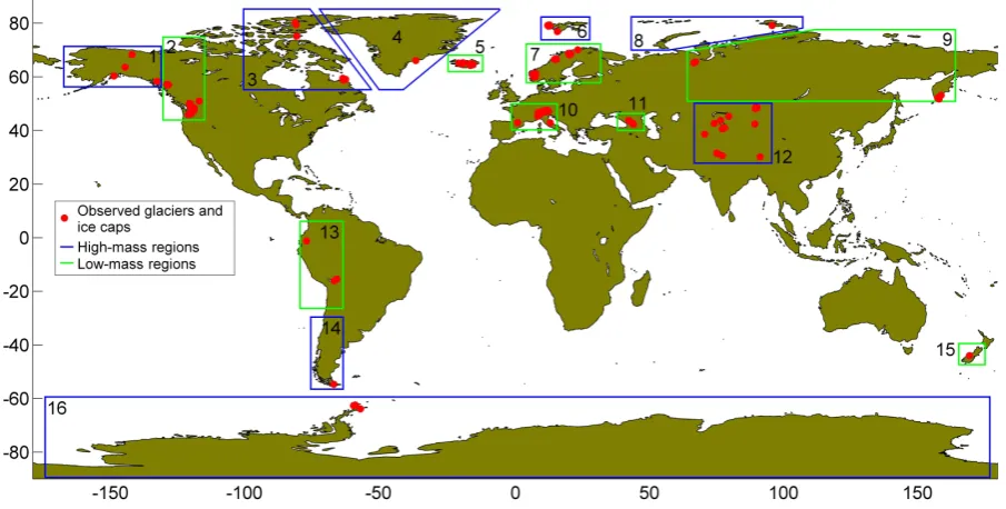
We compiled a data set of AAR (%) and mass balance (kg m−2yr−1) for 144 GIC (125 glaciers and 19 ice caps) from 1971 to 2010, mainly from the World Glacier Moni-toring Service (WGMS, 2012) but with additional data from Dyurgerov and Meier (2005), Bahr et al. (2009), and indi-vidual investigators. (See Sheet A in the supplementary ma-terial.) Thus we expanded and updated the data set used by BDM. We found that the BDM data set generally omits AARs for glaciers with net ablation at all elevations (hence AAR = 0) in a particular year. Including these values lowers the mean AAR. Figure 1 shows the locations of GIC in the updated data set, and Fig. 2 shows the number of GIC with AAR observations in each year.
These data were distilled from a larger data set that included several dozen additional glaciers in the WGMS database. For each glacier or ice cap we computed AAR0 by linear regression of the AAR with mass balance (Fig. 3 and Sheet B of the supplementary material). We retained only those GIC for which the linear relationship is statistically sig-nificant (p <0.10, based on a linear regressionttest) in or-der to remove GIC with short time series and those for which AAR methods are not applicable. Instances of AAR = 0 and AAR = 100 % were excluded from the regressions (but in-cluded for the broader analysis), since AAR and mass bal-ance are not related linearly when net ablation occurs at all elevations or when net accumulation occurs at all elevations. Following Dyurgerov et al. (2009), we assumed that AAR0 does not change in time.
We then computed annual, pentadal, and decadal averages of AAR andαfor selected regions (Fig. 1) and for the full data set, along with the fractional change in areapAand
vol-umepV required for GIC to reach equilibrium with a given
Fig. 1. Locations of the 144 glaciers and ice caps (GIC) in the updated data set. The data are divided into 16 regions: (1) Alaska, (2) western Canada/US, (3) Arctic Canada, (4) Greenland, (5) Iceland, (6) Svalbard, (7) Scandinavia, (8) the Russian Arctic, (9) North Asia, (10) central Europe, (11) the Caucasus, (12) central Asia, (13) the northern Andes, (14) the southern Andes, (15) New Zealand, and (16) Antarctica. The data set contains 38 GIC in high-mass regions (ice volumeV >5000 km3, outlined in blue) and 106 GIC in low-mass regions (V <5000 km3, outlined in green). Volume estimates are from Radi´c et al. (2013).
Fig. 2. Number of glaciers and ice caps with AAR observations per year in the Bahr et al. (2009) data set (black) and in the updated data set used in this study (grey).
future retreat if recent climate conditions continue, for 93 out of 96 GIC with observations during the 2000s. The mean AAR for 2001–2010 is 34±3 %. This is well below BDM’s estimate of 44±2 %, indicating that the observed GIC are farther from balance than previously reported. (Here and be-low, error ranges computed from our data set correspond to a 95 % confidence interval, or 1.96 times the standard error. Uncertainty ranges in other published work may not be di-rectly comparable. BDM, for example, expressed
uncertain-Fig. 3. Linear regression of AAR against mass balance for Silvretta Glacier, Swiss Alps. Theyintercept is AAR0, the equilibrium value of AAR. Each diamond represents one year of data.
ties as plus or minus one standard error, corresponding to a 68 % confidence interval.)
Fig. 4. Annual averageα= AAR / AAR0for the full data set (thin red line) and for the GIC in high-mass regions only (thin blue line), 1971–2010. The thick red and blue lines are 10 yr running means. Both the full data set and the high-mass-only data sets have signif-icant (p <0.01) negative trends during the periods 1971–2010 and 1991–2010. The 1971–1990 trends are not significant (p >0.10).
high-mass regions (each with an ice volumeV >5000 km3) and eight low-mass regions (V <5000 km3). The data set in-cludes 38 GIC in high-mass regions (Arctic Canada, Antarc-tica, Alaska, Greenland, the Russian Arctic, central Asia, Svalbard, and the southern Andes) and 106 GIC in low-mass regions (Iceland, western Canada/US, the northern Andes, central Europe, Scandinavia, North Asia, the Caucasus, and New Zealand). The high-mass regions collectively contain about 97 % of the Earth’s glacier mass.
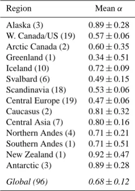
Area is not correlated significantly (p >0.10) with AAR orαfor observed GIC spanning a range of∼0.1 to 1000 km2 (Fig. 5), suggesting that glacier size is not a large source of bias. Geographic bias, on the other hand, could be important. In our data set, only 23 of 96 GIC with observed AAR dur-ing the period 2001–2010 are in high-mass regions. Table 1 shows the decadal meanαfor each of 14 regions with one or more GIC in the 2001–2010 data set. Among regions with at least three observed GIC, the highest values are in Alaska (α= 0.89±0.28) and Antarctica (α= 0.89±0.28), with the lowest values in Svalbard (α= 0.49±0.15) and central Eu-rope (α= 0.47±0.06). Three regions with low glacier mass (central Europe, Scandinavia, and western Canada/US) con-tain more than half the GIC in the data set and have relatively lowα. These regional differences suggest that the full data set may not be spatially representative and that projections based on the arithmetic meanαcould overestimate commit-ted GIC losses.
To show how geographical bias and undersampling can af-fect estimates of global glacier mass balance and AAR, we applied three different averaging methods: (1) the arithmetic mean for the full data set; (2) the arithmetic mean for the GIC in high-mass regions only; and (3) a mean obtained by
up-Fig. 5. Linear relation between the log of area (km2) and the 2001– 2010 meanα= AAR / AAR0for 96 GIC with observations in the past decade. Each diamond represents one glacier or ice cap. The correlation betweenαand the log of area, although slightly posi-tive (r2=0.03), is insignificant (p >0.10), suggesting that a bias toward smaller glaciers does not imply a bias inα.
Table 1. Regional mean values of α= AAR / AAR0 for 2001– 2010∗.
Region Meanα
Alaska (3) 0.89±0.28
W. Canada/US (19) 0.57±0.06 Arctic Canada (2) 0.60±0.35 Greenland (1) 0.34±0.51
Iceland (10) 0.72±0.09
Svalbard (6) 0.49±0.15
Scandinavia (18) 0.53±0.06 Central Europe (19) 0.47±0.06
Caucasus (2) 0.81±0.32
Central Asia (7) 0.80±0.16 Northern Andes (4) 0.71±0.21 Southern Andes (1) 0.71±0.51 New Zealand (1) 0.92±0.47 Antarctic (3) 0.89±0.28
Global (96) 0.68±0.12
∗Error ranges give 95 % confidence interval.
The number of observed GIC per region is shown in parentheses. The global mean is obtained by method 3.
scaling the regional mean values, with each value weighted by the region’s GIC area or volume. Because method 3 as-sumes GIC to be representative only of their regions and not of the entire Earth, it is the least likely to be geographically biased. This method, however, is limited to the past decade, because several high-mass regions had no observations in earlier decades.
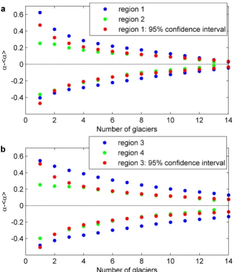
subsampling GIC in two well-represented regions – central Europe and western Canada/US – and computing the dif-ference between the meanα of each subsample and of the full sample (see Appendix B). The spread of differences as a function of subsample size (Fig. 6) gives an estimate of the errorδαin poorly sampled regions with small area (e.g., New Zealand, Caucasus, and Svalbard). For poorly sampled regions with large area (e.g., Greenland, Arctic Canada, the Russian Arctic, and Antarctica, whose glaciers experience different climate regimes within the region) we carried out the same analysis but using two combined regions: (1) cen-tral Europe and Scandinavia, and (2) western Canada/US and Alaska. All errors are derived as root-mean-square er-rors (RMSE) at 95 % confidence interval.
Figure 7 shows pentadal average global glacier mass bal-ance for 1971–2010 as estimated by each method (see Sheet D of the supplementary material), along with the estimates of Kaser et al. (2006), Cogley (2012), and Gardner et al. (2013). (No published benchmarks exist for global averageα. How-ever, α and mass balance are closely correlated, as shown in Fig. 8, suggesting that a method that is representative for mass balance is also representative for α.) The multi-decade time series in Fig. 7 show significant trends toward more negative mass balance. The estimates of Cogley (2012) are based on both geodetic and direct measurements and are more negative by 100–200 kg m−2yr−1than the direct-only estimates from Kaser et al. (2006), probably because the di-rect measurements exclude rapidly thinning calving glaciers (Cogley, 2009a). Gardner et al. (2013), who combined satel-lite observations with local glaciological measurements, es-timated a mass balance of−350±40 kg m−2yr−1for 2003– 2009, more than 100 kg m−2yr−1less negative than the other published estimates for the past decade. They found that lo-cal measurements tend to be negatively biased compared to satellite-based measurements.
Method 1 (the mean of all observed GIC) gives a post-2000 mass balance more negative than the published es-timates, suggesting a bias due to high melt rates in over-represented low-mass regions. Method 2 (the mean from high-mass regions) agrees closely with the direct-based es-timates of Kaser et al. (2006) and, as expected, gives a less negative mass balance than the direct-plus-geodetic esti-mates of Cogley (2012). Method 3 (based on regional upscal-ing) agrees closely with method 2 in 2001–2005 and 2006– 2010, but with large uncertainty ranges due to propagation of errors from undersampled high-mass regions. Both method 2 and method 3 give mass balances more negative than that of Gardner et al. (2013) during the past decade.
This comparison suggests that to a good approximation, methods 2 and 3 are globally representative for glacier mass balance (and hence α), but with two caveats. First, the direct-plus-geodetic results of Cogley (2012) imply that the exclusion of calving glaciers could result in a positive bias of 100 to 200 kg m−2yr−1. On the other hand, the re-sults of Gardner et al. (2013) suggest that mass loss
in-Fig. 6. Spread of decadal meanαas a function of subsample size in well-sampled regions. This plot shows the maximum difference between subsample meanαand referencehαias a function of the number of glaciers in the subsample for (a) two well-sampled re-gions: region 1, central Europe; and region 2, western Canada/US. (b) The same regions but extended: region 3, central Europe and Scandinavia; and region 4, western Canada/US and Alaska. The ref-erencehαiis the mean of the full sample, which includes glaciers with continuous AAR series during the period 2001–2010. In red is the difference range at 95 % confidence interval (1.96×standard deviation) for region 1 and region 3.
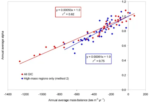
ferred from direct measurements is negatively biased com-pared to satellite measurements. The Gardner et al. (2013) estimate of 350±40 kg m−2yr−1 for 2003–2009 is 100 to 150 kg m−2yr−1 less negative than our method 2 and 3 estimates for the past decade. A mass-balance bias of 100 kg m−2yr−1 would be associated with biases of about 0.06 inpAand 0.08 inpV (Fig. 8).
3 Results and discussion
To estimate committed GIC area and volume losses based on present-day climate, we applied method 3 to observations of
α from 2001 to 2010. A window of about a decade is op-timal because it is long enough to average over interannual variability but short compared to glacier dynamic timescales. We adjusted for geographic bias by weighting each regional mean value by the region’s total GIC area (for computingpA)
Fig. 7. Pentadal average mass balance, 1971–2010. Estimated global average GIC mass balance (kg m−2yr−1)at 5 yr intervals from published estimates and from this data set: (1) Kaser et al. (2006), based on direct glacier measurements (purple); (2) Cog-ley (2012), based on direct plus geodetic measurements (yellow); (3) Gardner et al. (2013), with 95 % confidence interval for 2003– 2009 (black); (4) arithmetic mean of all GIC in the 1971–2010 data set (method 1, red); (5) arithmetic mean of GIC in the eight high-mass regions of Fig. 1 (method 2, blue); (6) average based on area-weighted upscaling of regional means (method 3, green) including error bars at 95 % confidence interval.
Errors were estimated based on the number of observed GIC per region, and are dominated by a few underrepresented re-gions (see Appendix B). We foundα= 0.68±0.12 for 2001– 2010, implying committed area losses of 32±12 % and vol-ume losses of 38±16% if climate conditions of 2001–2010 continue in the future. The resulting sea-level rise scales lin-early with the initial glacier volume. Assuming a total GIC volume of 430 mm sea-level equivalent (SLE) (Huss and Farinotti, 2012), these committed glacier losses would raise global mean sea level by 163±69 mm. Using a larger value of 522 mm SLE (Radi´c et al., 2013), global mean sea level would rise by 198±84 mm.
Method 2 yields similar estimates. The mean α dur-ing the period 2001–2010 for GIC in high-mass regions is 0.70±0.10, implying committed area losses of 30±10 % and volume losses of 37±12 % (where the error estimates are based on the assumption that these GIC are globally rep-resentative). The close agreement with method 3 suggests that method 2 does not have a large geographic bias with respect toα.
The Earth is expected to warm further (e.g., Meehl et al., 2007), making it likely that long-term GIC area and vol-ume losses will exceed estimates based on the climate of the past decade. From method 2, there is a significant neg-ative trend (p <0.01, based on attest) in average annualα
of−0.0052±0.0033 yr−1 from 1971 to 2010 (Fig. 4). The trend is nearly identical for the subset of GIC with observa-tions in all four decades, implying that the changing
com-Fig. 8. Linear relation between average mass balance and average αfor the period 1971–2010. Each diamond represents the average of all GIC observations for one year. The red diamonds denote av-erages over the full data set, and the blue diamonds denote avav-erages over the GIC in high-mass regions only. The regression lines are forced to pass through the point(x, y)= (0, 1). Both correlations are significant (p <0.01), as determined from the squared correla-tion coefficient,r2. A change in mass balance of 100 kg m−2yr−1 is associated with a change inαof about 0.06.
position of the data set does not substantially bias the trend. The trend inα has been much steeper since 1990; there is a significant negative trend (p <0.01, based on at test) of −0.0078±0.0082 yr−1 for 1991–2010, whereas the 1971– 1990 trend is not significantly different from zero (p >0.10). By extrapolating these trends, we can estimate the losses required to equilibrate with the climate of future decades. Takingα=0.68±0.12 as the 2005 value and extending the 40 yr trend, the average would fall by 0.18±0.12 over 35 yr, reaching 0.50±0.17 by 2040. The Earth’s GIC would then be committed to losing 50±17 % of their area and 60±20 % of their volume (see Appendix A). Relative to present-day GIC volume, which is decreasing by about 2 % per decade, the losses would be somewhat greater. These error ranges may understate the true uncertainties because of natural in-terdecadal variability, and because the method 2 data set may not be globally representative.
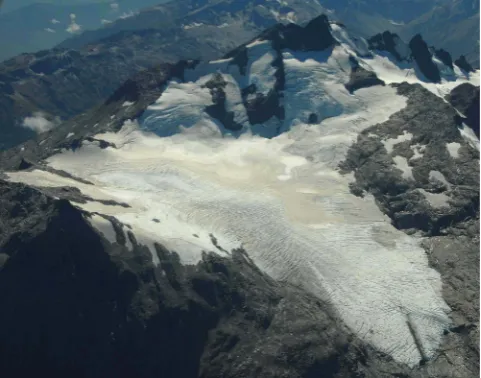
Fig. 9. Brewster Glacier, New Zealand, at the end of the 2008 ab-lation season. The glacier area is 2.5 km2. The 2008 glacier mass balance is−1653 kg m−2yr−1, and the AAR is 10 %, with net ac-cumulation limited to small white patches of remaining snow. Grey firn areas (i.e., snow from previous years) generally lie in the ab-lation zone, as does the bare (blue) ice. The photo illustrates the difficulty of determining a specific elevation at which a glacier is in equilibrium. Photo taken by A. Willsman (Glacier Snowline Survey, National Institute of Water and Atmospheric Research Ltd (NIWA), New Zealand), 14 March 2008.
This analysis has focused on global ice losses and sea-level rise, but glacier retreat and thinning will also have re-gional impacts associated with changes in seasonal runoff (Immerzeel et al., 2010; Kaser et al., 2010) and glacier haz-ards (Kääb et al., 2005). In some regions, fractional area and volume ice losses will exceed the global average. As-suming that the observed GIC are regionally representative, GIC in central Europe will lose 64±7 % of their volume if future climate resembles the climate of the past decade (which included several record heat waves). We also project substantial volume losses in Scandinavia (56±7 %), west-ern Canada/US (53±7 %) and Iceland (35±11 %). Projec-tions elsewhere are less certain because of the smaller sample sizes.
4 Conclusions
AARs are declining faster than most glaciers and ice caps (GIC) can respond dynamically. As a result, committed area and volume losses far exceed the losses observed to date. Based on regional upscaling of AAR observations from 2001 to 2010, we conclude that the Earth’s glaciers and ice caps will ultimately lose 32±12 % of their area and 38±16 % of their volume if the future climate resembles the climate of the past decade. Committed losses could increase substantially during the next few decades if the climate continues to warm.
These relative losses are larger than those estimated by BDM, reflecting the lower AARs in data that have become available since the earlier study. Our projections, however, have large uncertainties (40 % relative error in the projected mass loss) that are dominated by underrepresented high-mass regions, including Arctic Canada, Antarctica, Greenland, and Alaska. To reduce the uncertainties, more observations are needed in poorly sampled regions. Direct mass-balance and AAR measurements are inherently labor intensive and limited in coverage. AARs can be estimated, however, from aerial and satellite observations of the end-of-summer snowline (e.g., Fig. 9 and Rabatel et al., 2013). Deriving AAR0 from ob-servations requires mass-balance measurements for about a decade, but BDM found that the global mean AAR0 can be used for most GIC with only moderate loss of precision. Huss et al. (2013) recently showed that simple mass balance modeling, combined with terrestrial and airborne/spaceborne AAR observations, can be used to determine glacier mass changes. Also, AAR methods could be extended to tidewater glaciers, incorporating calving as well as surface processes.
Appendix A
Means and errors ofα,pA, andpV
The first section of Sheet C in the supplementary material (All GIC – alpha,pA,pV) shows values ofα= AAR / AAR0
for the full data set. For each yeari, the annual meanαis found by averaging overNi values:
¯
αi = Ni
P
n=1
αni
Ni
, (A1)
whereαnidenotes the value for glaciernin yeari. The
vari-ance for each year is computed as
σi2= 1
Ni−1 Ni
X
n=1
(αni− ¯αi)2, (A2)
resulting in a standard error of
δαi =
σi
√
Ni
. (A3)
The annual values and running 10 yr means are shown in Fig. 4.
Arithmetic means for the full data set were computed for four 10 yr windows: 1971–1980, 1981–1990, 1991–2000, and 2001–2010. For the full data set we computed a mean
αof 0.93±0.06, 0.85±0.06, 0.83±0.07, and 0.59±0.05 during the 1970s, 1980s, 1990s, and 2000s, respectively. Let us suppose that for a given glaciern, we have measurements inMnout of 10 yr (1≤Mn≤10). In order for each
Fig. A1. Correlation betweenαtime series (2001–2010) of any two glaciers in a region versus the distance between the two glaciers. (a) Region 3: central Europe (15 glaciers) and Scandinavia (5 glaciers); (b) region 4: western Canada/US (14 glaciers) and Alaska (2 glaciers).
¯
α=
N
P
n=1
fnα¯n
Nf
, (A4)
wherefn=Mn/10,α¯nis given by
¯
αn= Mn
P
i=1
αni
Mn
, (A5)
and
Nf =
N
X
n=1
fn. (A6)
Equation (A4) is equivalent to the arithmetic mean of all measurements, with each measurement weighted equally. We can think ofNf as the equivalent number of glaciers; it is
equal to the total number of measurements divided by the number of years. The variance is given by
σ2= 1
Nf −1 N
X
n=1
fn(α¯n− ¯α)2, (A7)
and the standard error is
δα= σ
p Nf
. (A8)
The arithmetic mean AAR and its standard error, shown in the second section of Sheet C for 2001–2010 only, are com-puted analogously.
The next sections of Sheet C show the 2001–2010 arith-metic mean values ofpAandpV for the full data set. BDM
showed that for a given glacier or ice cap,pA=α−1 and
pV =αγ−1, whereα= AAR / AAR0andγ is the exponent in the glacier volume–area scaling relationship, V =cAγ
(Bahr et al., 1997). Data and theory suggestγ =1.25 for ice caps andγ =1.375 for glaciers. ThuspV depends onγ but
not on the poorly constrained constantc, andpAis
indepen-dent of bothcandγ. We compute means ofpAandpV first
for glaciers, then separately for ice caps. (In the text below, we generally refer to “glaciers”, but the same analysis ap-plies to ice caps with the appropriate value ofγ.) For a single glacier we havep¯An= ¯αn−1 andp¯V n= ¯αγn−1, whereα¯n
is the mean value ofαfor glaciernover the decade. Let us suppose we have at least oneαvalue during the decade for each ofN glaciers. To give greater weight to glaciers with more measurements, we compute the decadal meanp¯A and
¯
pV as
¯
pA= N
P
n=1
fnα¯n
Nf
−1 (A9)
and
¯
pV = N
P
n=1
fnαγn
Nf
−1. (A10)
The variance associated withpAis
σp2
A= 1
Nf −1 N
X
n=1
fn(α¯n− ¯α)2, (A11)
and the variance associated withpV is
σp2
V = 1
Nf−1 N
X
n=1
fn(α γ
n−αγ)2. (A12)
The standard errors are
δpA=
σpA
p Nf
(A13)
and
δpV =
σpV
p Nf
. (A14)
must lose 44±6 % of their area and 51±7 % of their vol-ume, and ice caps must lose 32±9 % of their area and 38±10 % of their volume, in order to reach equilibrium with the climate of the past decade. As discussed in the main text, however, the data are likely to be geographically biased.
To assess the data for size biases, we plotted the mean value ofα for each glacier against the log of glacier area. As shown in Fig. 5, the correlation is slightly positive (r2= 0.03) but statistically insignificant (p <0.10). The correla-tion betweenαand glacier area is also insignificant. A pos-itive correlation between glacier area and the change in α
(relative to the equilibrium value of 1.0) would be expected in the following case: if (1) larger glaciers have greater ele-vation ranges than smaller glaciers; (2) for a given lifting of the equilibrium line altitude (ELA), the AAR decreases less for glaciers with large elevation ranges than for glaciers with small elevation ranges; and (3) the average lifting of the ELA in a warming climate is independent of glacier size. The lack of a significant correlation between glacier area andα sug-gests that one or more of these assumptions does not apply to the observed GIC. We checked for area-range bias (i.e., the first assumption) by comparing plots of glacier area vs. el-evation range for (1) the observed GIC and (2) more than 100 000 GIC in the World Glacier Inventory (Cogley et al., 2009b). We did not find evidence of a significant bias.
Sheet E in the supplementary material (High mass regions) is similar to Sheet C except that it includes only the 38 GIC in high-mass regions: Arctic Canada, Antarctica, Alaska, Greenland, the Russian Arctic, central Asia, Svalbard, and the southern Andes. The first three sections show AAR, mass balance, andα, respectively. Decadal mean values ofα,pA,
andpV as well as the associated standard errors are shown
for 2001–2010. These are the “method 2” averages cited in the text. The arithmetic mean and 10 yr running mean are shown in Fig. 4, and the 40 yr linear trend (1971–2010) and two 20 yr linear trends (1971–1990 and 1991–2010) of the mean values are given in Sheet E. We used a t test to de-termine significance. The 1970–2009 and 1990–2009 trends are significantly negative at the 1 % level, whereas the 1970– 1989 trend is not significantly different from zero at the 10 % level. In the last section of Sheet E, we repeated the annual mean and trend calculations for the 11 GIC in high-mass re-gions with observations in all four decades to assess the ef-fect on the trends of the changing composition of the data set. The trends are similar to those computed for all 38 GIC.
To estimate future values of the global meanα, we took
αglobal=0.68±0.12 (the global mean value estimated for 2001–2010, given in Section 3) as a best estimate for 2005. We applied the 40 yr trend (−0.0052±0.0033 yr−1) given in Sheet E for the 38 high-mass GIC (method 2). Extending this trend for 35 yr gives a change of−0.18±0.12, resulting in
αglobal= 0.50±0.17 by 2040. (It is possible that the down-ward trend inα would slow asαreaches 0 for an increas-ing number of glaciers. With this 35 yr mean trend, however, only three of 96 glaciers with data in 2001–2010 would have
α=0 by 2040, with a negligible effect on the results.) We setpVglobal= α¯global
¯
γ
−1, withγ¯=1.31±0.05 to reflect an uncertain partitioning of volume between glaciers and ice caps. The errorδP vglobal=0.20 was calculated as
(δpV)2=
∂pV
∂α 2
¯
α
(δα)2+
∂pV
∂γ 2
¯
γ
(δγ )2. (A15)
Appendix B
Regional calculations
Sheet F (Regional mass balance) shows the average mass balance during the period 2001–2010 for each of 14 regions (Table 1), the estimated GIC area in the region (Radi´c et al., 2013), and the corresponding fraction of the Earth’s total GIC area. For the past decade the data set has no observations from the Russian Arctic, which contains an estimated 8 % of global GIC area, or from North Asia, which contains much less than 1 %. For purposes of regional upscaling, we used Svalbard (which is climatically similar) as a surrogate for the Russian Arctic, and we neglected North Asia. Thus the re-gional area fractions are relative to a global total that omits the small GIC area in North Asia. The global average mass balance is computed as
bglobal=
X
n
wAnbn, (B1)
wherewAn is the fractional area weight for regionn, andbn
is the mean mass balance. Sheet F shows the global aver-age mass balance computed for the full decade, for each of two pentads, and for the period 2003–2009 (corresponding to Gardner et al., 2013).
Sheet G (Regional alpha) shows regional mean values of
αin 2001–2010 for the same 14 regions (Table 1 in the main text) based on Radi´c et al. (2013). Again, Svalbard is used as a surrogate for the Russian Arctic, and North Asia is ne-glected. Decadal mean α for each glacier and ice cap are shown in Sheet G. Measurements of α are averaged, with each measurement weighted equally, to obtain the regional meansα¯n. The estimated area and volume losses per region
arep¯An= ¯αn−1 andp¯V n=(α¯n)γ¯n−1, whereγ¯nis estimated
as described below. The upscaled global estimates are ob-tained by summing over regions, with each regional value weighted by the estimated total GIC area in the region (forα
andpA) and total volume (forpV):
pAglobal=
X
n
wAnp¯An, (B2)
pVglobal=
X
n
wV np¯V n. (B3)
The upscaled values, with errors, are shown in Sheet G. The regional area and volume weights, wAn andwV n, are also
The errors for these global estimates are given by
δpAglobal2=
X
n
(wAnδpAn)2, (B4)
δpVglobal 2
=X
n
(wV nδpV n)2, (B5)
whereδpAn andδpV n are the regional errors. For each
re-gion we have δpAn=δαn, where δαn (shown in column
V) is estimated by the following method. We subsampled GIC in two well-represented regions, central Europe and western Canada/US. For 2001–2010 we consideredn=15 glaciers with continuous records in central Europe, andn= 14 glaciers with continuous records in western Canada/US. The full samples per region provide reference mean values hαifor each region. For each region we computed means for all possible subsamples containing 1 ton−1 glaciers. For a subsample of one glacier, regionalαis equal toαfrom each glacier, and therefore this subsample gives the largest range of possible values. We also calculated the regional meanα
for all possible subsamples of two glaciers, three glaciers, and so on. For each subsample size, Fig. 6a shows the maxi-mum range of results (i.e., subsampled regionalαminus the referencehαi). The range is largest for a subsample of one glacier and slowly decreases as we approach the maximum of 14 glaciers (and would reach zero for the total of 20 in this case). For each subsample size we computed the standard de-viation of theαvalues. Figure 6a shows the 95 % confidence interval (1.96×standard deviation), which provides an esti-mate ofδαnin poorly sampled regions with small spatial area
(Iceland, Svalbard, the northern Andes, the Caucasus, and New Zealand). For regions containing more than 10 glaciers with observed AAR (central Europe, Scandinavia and west-ern Canada/US) we assigned an error based on a subsample size of 12. (A number>10 was chosen arbitrarily, but the error does not decline significantly for sample sizes >10; any number from 11 to 14 would give a similar error estimate.) Based on the data from central Europe, which has a wider spread of differences than western Canada/US, the errors (values ofn shown in parentheses) are as follows: Iceland (10),δα=0.09; Svalbard (6),δα=0.15; the northern An-des (4),δα=0.21; Caucasus (2), δα=0.32; New Zealand (1), δα=0.47; and central Europe (19), Scandinavia (18), and western Canada/US (18),δα=0.06.
For poorly sampled regions covering large spatial area (central Asia, Alaska, Antarctica, Arctic Canada, the south-ern Andes, and Greenland), we carried out the same anal-ysis but using two combined regions: (1) central Europe and Scandinavia, and (2) western Canada/US and Alaska (Fig. 6b). Thus, in addition to n=15 glaciers from cen-tral Europe we included n=5 glaciers from Scandinavia, and in addition ton=14 glaciers from western Canada/US we includedn=2 glaciers from Alaska. For each of these two extended regions we carried out a correlation analysis.
Although there are a few correlations of∼0.5 for glaciers
>1500 km apart, most time series ofαare not significantly correlated when the distance between glaciers exceeds∼300 km (Fig. A1). Therefore, the glacier sampling in the com-bined regions is representative for poorly sampled regions covering large spatial areas whose glaciers experience dif-ferent climatic regimes within the region. Based on the data from central Europe and Scandinavia (which has a wider spread of differences than western Canada/US and Alaska), the errors at 95 % confidence interval (values of n shown in parentheses) are as follows: central Asia (7),δα=0.16; Alaska and Antarctica (3), δα=0.28; Arctic Canada (2),
δα=0.35; and Greenland and the southern Andes (1),δα= 0.51.
SincepV is a function of bothαandγ, the regional errors
δpV ndepend on bothδαnandδγn:
(δpV n)2=
∂p V ∂α 2 ¯ αn
(δαn)2+
∂p V ∂γ 2 ¯ γn
(δγn)2, (B6)
whereα¯ andγ¯are best estimates. Evaluating the derivatives, this becomes
(δpV n)2=
¯
γnα¯
¯
γ−1
n
2
(δαn)2+
¯
αγn¯ln(α¯n)
2
(δγn)2. (B7)
We estimatedγ¯nandδγnas follows. Drawing from existing
glacier inventories (Cogley, 2009b), we tabulated the total number of GIC and the number of ice caps in each region. Regions with relatively few ice caps (less than 1 % of the to-tal number of GIC in the regional inventory) were assumed to have most of their volume contained in glaciers. For these regions we assumedγ¯ =1.36±0.02, where the error corre-sponds roughly to the difference between the observed value of 1.36 for valley glaciers and the theoretical value (Bahr et al., 1997) of 1.375. For regions where at least 1 % of the GIC are classified as ice caps, we assumedγ¯=1.31±0.05 to reflect an uncertain partitioning of volume between glaciers and ice caps. (Because ice caps can be much larger than typi-cal glaciers, a relatively small number of ice caps can contain a substantial fraction of a region’s volume. BDM, for exam-ple, estimated that 53 % of total GIC volume is contained in ice caps and 47 % in glaciers, although there are many more glaciers than ice caps.) A more complete analysis would use scaling relationships to estimate the total glacier and ice cap volume in each region. Existing inventories, however, do not contain complete lists of glaciers and ice caps in all regions, nor do all GIC fall clearly into one category or the other.
Although the partitioning between glaciers and ice caps is only approximate, our results are not sensitive to the de-tails of this partitioning. The errorsδpV nare dominated by
the term containingδαn(the first term on the right-hand side
of Eq. B6), with much smaller contributions from the term containing δγn (the second term on the right-hand side of
Appendix C
Glacier volume response times
The volume response time for a glacier, defined as the timescale for exponential adjustment to a new steady-state volume following a mass-balance perturbation, can be esti-mated asτV ∼H /|bT|, where H is a thickness scale (e.g., mean glacier thickness) andbTis the mass balance at the ter-minus (Jóhannesson et al., 1989). For typical glaciers with thicknesses of 100 to 500 m and terminus melt rates of 1 to 5 m yr−1, the response time is on the order of 100 yr. The mean terminus melt rate for our data set is∼3 m yr−1, as shown in Sheet I (Terminus mass balance).
Bahr and Radi´c (2012) showed that the fraction of total volume contained in glaciers of area less thanAminis given to a good approximation by
2=
A
min
Amax
γ−β+1
, (C1)
whereAmaxis the area of the largest glaciers;γ=1.375 is the exponent in the volume–area scaling relationship V ∝
Aγ; andβ=2.1 is the exponent in the power lawN (A)∝
A−β, which predicts the number of glaciers N of size A. Volume–area scaling impliesh∝Aγ−1, wherehis the mean ice thickness. Therefore,
2=
hmin
hmax
γ−γ−β+11
. (C2)
The largest glaciers and ice caps have a thickness of about 1000 m. Settinghmin=500 m and hmax=1000 m in Eq. (A24), we obtain2=0.60, implying that approximately 60 % of total glacier volume resides in glaciers thinner than 500 m. This analysis suggests that glaciers with response times on the order of a century or less contain a majority of the Earth’s total glacier volume.
Appendix D
Contributing investigators
The principal investigators for the glaciers and ice caps in the WGMS database are listed in WGMS (2012) and earlier bul-letins. We have supplemented the WGMS database with data compiled by Mark Dyurgerov (Dyurgerov et al., 2005; Bahr et al., 2009). In addition, we thank the following investiga-tors for providing us with data not previously in the WGMS database:
– Pedro Skvarca: Bahia Del Diablo
– Andrea Fischer and Gerhard Markl: Hintereisferner,
Jamtalferner, Kesselwandferner
– Heinz Slupetzky: Sonnblickkees
– Ludwig N. Braun: Vernagtferner
– Reinhard Böhm and Wolfgang Schöner:
Gold-bergkees, Kleinfleißkees, Wurtenkees
– Javier C. Mendoza Rodríguez and Bernard Francou:
Charquini Sur, Zongo
– Alex Gardner: Devon Ice Cap NW
– Graham Cogley: White
– Bolívar Cáceres Correa and Bernard Francou:
Anti-zana 15 Alpha
– Niels Tvis Knudsen: Mittivakkat
– Finnur Pálsson, Helgi Björnsson, and Hannes Haralds-son: Brúarjökull, Eyjabakkajökull, Köldukvíslarjökull,
Langjökull S. Dome, Tungnaárjökull
– Þorsteinn Þorsteinsson: Hofsjökull N, Hofsjökull E,
Hofsjökull SW
– Luca Carturan: Carèser
– Luca Mercalli: Ciardoney
– Gian Carlo Rossi and Gian Luigi Franchi: Malavalle,
Pendente
– Bjarne Kjøllmoen: Ålfotbreen, Breidalblikkbrea,
Gråf-jellsbrea, Langfjordjøkelen, Nigardsbreen
– Hallgeir Elvehøy: Austdalsbreen, Engabreen,
Hardan-gerjøkulen
– Liss M. Andreassen: Gråsubreen, Hellstugubreen,
Storbreen
– Jack Kohler: Austre Brøggerbreen, Kongsvegen,
Midtre Lovénbreen
– Piotr Glowacki and Dariusz Puczko: Hansbreen
– Ireneusz Sobota: Waldemarbreen
– O.V. Rototayeva: Garabashi
– Yu K. Narozhniy: Leviy Aktru, Maliy Aktru, and No.
125
– Miguel Arenillas: Maladeta
– Peter Jansson: Mårmaglaciären, Rabots glaciär,
Riukojietna, Storglaciären
– Giovanni Kappenberger and Giacomo Casartelli:
Basòdino
– Mauri Pelto: Columbia (2057), Daniels, Easton, Foss,
Ice Worm, Lower Curtis, Lynch, Rainbow, Sholes, Yawning, Lemon Creek
– Jon Riedel: Noisy Creek, North Klawatti, Sandalee,
Silver
– Rod March and Shad O’Neel: Gulkana, Wolverine
– William R. Bidlake: South Cascade
Supplementary material related to this article is available online at http://www.the-cryosphere.net/7/ 1565/2013/tc-7-1565-2013-supplement.zip.
Acknowledgements. We thank principal investigators and their teams, along with the WGMS staff, for providing AAR and mass-balance data. We also thank Daniel Farinotti, Ben Marzeion, and Mauri Pelto for insightful reviews, and we thank Graham Cogley, Alex Gardner, Matthias Huss, and Georg Kaser for helpful data and feedback. This work was supported partly by a Los Alamos National Laboratory (LANL) Director’s Fellowship and by the Earth System Modeling program of the Office of Biological and Environmental Research within the US Department of Energ’s Office of Science. LANL is operated under the auspices of the National Nuclear Security Administration of the US Department of Energy under contract No. DE-AC52-06NA25396, and partly by the European Community’s Seventh Framework Programme under grant agreement No. 262693.
Edited by: J. O. Hagen
References
Arendt, A. A., Bolch, T., Cogley, J. G., Gardner, A., Hagen, J.-O., Hock, R., Kaser, G., Pfeffer, W. T., Moholdt, G., Paul, F., Radi´c, V., Andreassen, L., Bajracharya, S., Beedle, M., Berthier, E., Bhambri, R., Bliss, A., Brown, I., Burgess, E., Burgess, D., Cawkwell, F., Chinn, T., Copland, L., Davies, B., de Angelis, H., Dolgova, E., Filbert, K., Forester, R., Fountain, A., Frey, H., Giffen, B., Glasser, N., Gurney, S., Hagg, W., Hall, D., Hari-tashya, U. K., Hartmann, G., Helm, C., Herreid, S., Howat, I., Kapustin, G., Khromova, T., Kienholz, C., Koenig, M., Kohler, J., Kriegel, D., Kutuzov, S., Lavrentiev, I., LeBris, R., Lund, J., Manley, W., Mayer, C., Miles, E., Li, X., Menounos, B., Mer-cer, A., Moelg, N., Mool, P., Nosenko, G., Negrete, A., Nuth, C., Pettersson, R., Racoviteanu, A., Ranzi, R., Rastner, P., Rau, F., Rich, J., Rott, H., Schneider, C., Seliverstov, Y., Sharp, M., Sigurðsson, O., Stokes, C., Wheate, R., Winsvold, S., Wolken, G., Wyatt, F., and Zheltyhina, N: Randolph Glacier Inventory [v2.0]: a Dataset of Global Glacier Outlines, digital media, avail-able at: http://www.glims.org/RGI/RGI_Tech_Report_V2.0.pdf, Global Land Ice Measurements from Space, Boulder, Colorado, 2012.
Bahr, D. B. and Radi´c, V.: Significant contribution to total mass from very small glaciers, The Cryosphere, 6, 763–770, doi:10.5194/tc-6-763-2012, 2012.
Bahr, D. B., Meier, M. F., and Peckham, S. D.: The physical basis of glacier volume-area scaling, J. Geophys. Res., 102, 20355– 20362, 1997.
Bahr, D. B., Dyurgerov, M., and Meier, M. F.: Sea-level rise from glaciers and ice caps: A lower bound, Geophys. Res. Lett., 36, L03501, doi:10.1029/2008GL036309, 2009.
Cazenave, A. and Llovel, W.: Contemporary sea level rise, Annu. Rev. Mar. Sci., 2, 145–173, 2010.
Cogley, J. G.: Geodetic and direct mass-balance measurements: comparison and joint analysis, Ann. Glaciol., 50, 96–100, 2009a. Cogley, J. G.: A more complete version of the World Glacier
Inven-tory, Ann. Glaciol., 50, 32–38, 2009b.
Cogley, J. G.: The Future of the World’s Glaciers, in: The Future of the World’s Climate, edited by: Henderson-Sellers, A. and McGuffie, K., 197–222, Elsevier, Amsterdam, 2012.
Dyurgerov, M. B.: Data of Glaciological Studies – Reanalysis of Glacier Changes: From the IGY to the IPY, 1960–2008, Publica-tion No. 108, Institute of Arctic and Alpine Research, Boulder, Colorado, 2010.
Dyurgerov, M. B. and Meier, M. F.: Glaciers and the Changing Earth System: A 2004 Snapshot, Occas. Paper 58, 117 pp., Institute of Arctic and Alpine Research, Boulder, Colorado, 2005.
Dyurgerov, M. B., Meier, M. F., and Bahr, D. B.: A new index of glacier area change: a tool for glacier monitoring, J. Glaciol., 55, 710–716, 2009.
Gardner, A. S., Moholdt, G., Cogley, J. G., Wouters, B., Arendt, A. A., Wahr, J., Berthier, E., Hock, R., Pfeffer, W. T., Kaser, G., Ligtenberg, S. R. M., Bolch, T., Sharp, M. J., Hagen, J. O., van den Broeke, M. R., and Paul, F. A: Reconciled estimate of glacier contributions to sea level rise: 2003 to 2009, Science, 340, 852– 857, 2013.
Huss, M. and Farinotti, D.: Distributed ice thickness and volume of all glaciers around the world, J. Geophys. Res., 117, F04010, doi:10.1029/2012JF002523, 2012.
Huss, M., Sold, L., Hoelzle, M., Stokvis, M., Salzmann, N., Farinotti, D., and Zemp, M.: Towards remote monitoring of sub-seasonal glacier mass balance, Ann. Glaciol., 54, 85–93, doi:10.3189/2013AoG63A427, 2013.
Immerzeel, W. W., van Beek, L. P. H., and Bierkens, M. F. P.: Cli-mate change will affect the Asian water towers, Science, 328, 1382–1385, 2010.
Jacob, T., Wahr, J., Pfeffer, W. T., and Swenson, S.: Recent con-tributions of glaciers and ice caps to sea level rise, Nature, 482, 514–518, 2012.
Jóhannesson, T., Raymond, C., and Waddington, E.: Time-scale for adjustment of glaciers to changes in mass balance, J. Glaciol., 35, 355–369, 1989.
Kääb, A., Reynolds, J. M., and Haeberli, W.: Glacier and permafrost hazards in high mountains, in: Global Change and Mountain Re-gions: An Overview of Current Knowledge, edited by: Huber, U. M., Bugmann, H. K. M., and Reasoner, M. A., Springer, Dor-drecht, the Netherlands, 225–234, 2005.
Kaser, G., Großhauser, M., and Marzeion, B.: Contribution potential of glaciers to water availability in different climate regimes, P. Natl. Acad. Sci. USA, 107, 20223–20227, 2010.
Marzeion, B., Jarosch, A. H., and Hofer, M.: Past and future sea-level change from the surface mass balance of glaciers, The Cryosphere, 6, 1295–1322, doi:10.5194/tc-6-1295-2012, 2012. Meehl, G. A. and Stocker, T. F.: Global climate projections, in:
Cli-mate Change 2007: The Physical Science Basis, Contribution of Working Group I to the Fourth Assessment Report of the Inter-governmental Panel on Climate Change, edited by: Solomon, S., Qin, D., Manning, M., Marquis, M., Averyt, K., Tignor, M. M. B., Miller Jr., H. L., and Chen, Z., Cambridge University Press, Cambridge, 2007.
Meier, M. F., Dyurgerov, M. B., Rick, U. K., O’Neel, S., Pfeffer, W. T., Anderson, R. S., Anderson, S. P., and Glazovsky, A. F.: Glaciers dominate eustatic sea-level rise in the 21st century, Sci-ence, 317, 1064–1067, 2007.
Oerlemans, J., Anderson, B., Hubbard, A., Hybrechts, P., Jóhannes-son, T., Knap, W. H., Schmeits, M., Stroeven, A. P., van de Wal, R. S. W., Wallinga, J., and Zuo, Z.: Modelling the response of glaciers to climate warming, Clim. Dynam., 14, 267–274, 1998. Pelto, M. S.: Forecasting temperate alpine glacier survival from accumulation zone observations, The Cryosphere, 4, 67–75, doi:10.5194/tc-4-67-2010, 2010.
Rabatel, A., Letréguilly, A., Dedieu, J.-P., and Eckert, N.: Changes in glacier Equilibrium-Line Altitude (ELA) in the western Alps over the 1984–2010 period: evaluation by remote sensing and modeling of the morpho-topographic and climate controls, The Cryosphere Discuss., 7, 2247–2291, doi:10.5194/tcd-7-2247-2013, 2013.
Radi´c, V. and Hock, R.: Regionally differentiated contribution of mountain glaciers and ice caps to future sea-level rise, Nat. Geosci., 4, 91–94, 2011.
Radi´c, V., Bliss, A., Breedlow, A. C., Hock, R., Miles, E., and Cog-ley, J. G.: Regional and global projections of twenty-first cen-tury glacier mass changes in response to climate scenarios from global climate models, Clim. Dynam., doi:10.1007/s00382-013-1719-7, 2013.
Raper, S. C. B. and Braithwaite, R. J.: Low sea level rise projec-tions from mountain glaciers and icecaps under global warming, Nature, 439, 311–313, 2006.
Slangen, A. B. A., Katsman, C. A., van de Wal, R. S. W., Ver-meersen, L. L. A., and Riva, R. E. M.: Towards regional pro-jections of twenty-first century sea-level change based on IPCC SRES scenarios, Clim. Dynam., 38, 1191–1209, 2012.