The Cryosphere, 7, 1857–1867, 2013 www.the-cryosphere.net/7/1857/2013/ doi:10.5194/tc-7-1857-2013
© Author(s) 2013. CC Attribution 3.0 License.
The Cryosphere
Open Access
Interferometric swath processing of Cryosat data for glacial ice
topography
L. Gray1, D. Burgess2, L. Copland1, R. Cullen3., N. Galin4, R. Hawley5, and V. Helm6
1Department of Geography, University of Ottawa, Ottawa, Canada 2Geological Survey of Canada, NRCan, Ottawa, Canada
3Vega Space Ltd., Hertfordshire., UK
4Laboratory for Satellite Altimetry, NOAA, MD 20740, USA
5Department of Earth Sciences, Dartmouth College, Hanover, NH, USA
6Helmholtz Centre for Polar and Marine Research, Alfred Wegener Institute, Bremerhaven, Germany Correspondence to: L. Gray ([email protected])
Received: 9 June 2013 – Published in The Cryosphere Discuss.: 27 June 2013
Revised: 23 October 2013 – Accepted: 28 October 2013 – Published: 12 December 2013
Abstract. We have derived digital elevation models (DEMs)
over the western part of the Devon Ice Cap in Nunavut, Canada, using “swath processing” of interferometric data collected by Cryosat between February 2011 and January 2012. With the standard ESA (European Space Agency) SARIn (synthetic aperture radar interferometry) level 2 (L2) data product, the interferometric mode is used to map the cross-track position and elevation of the “point-of-closest-approach” (POCA) in sloping glacial terrain. However, in this work we explore the extent to which the phase of the re-turns in the intermediate L1b product can also be used to map the heights of time-delayed footprints beyond the POCA. We show that there is a range of average cross-track slopes (∼0.5 to∼2◦) for which the returns will be dominated by those beneath the satellite in the main beam of the antenna so that the resulting interferometric phase allows mapping of heights in the delayed range window beyond the POCA. In this way a swath of elevation data is mapped, allowing the creation of DEMs from a sequence of L1b SARIn Cryosat data takes. Comparison of the Devon results with airborne scanning laser data showed a mean difference of order 1 m with a standard deviation of about 1 m. The limitations of swath processing, which generates almost 2 orders of magni-tude more data than traditional radar altimetry, are explored through simulation, and the strengths and weaknesses of the technique are discussed.
1 Introduction
Surface elevation data for ice caps and glaciers derived from satellite altimetry have been used to produce both surface el-evation DEMs (digital elel-evation models; e.g. Bamber et al., 2009) and measurements of surface elevation change (e.g. Zwally and Giovinetto, 2011). The estimation of surface el-evation change forms the basis of one of three remote sens-ing methodologies for calculatsens-ing ice sheet and glacier mass balance information (Shepherd et al., 2012; Gardelle et al., 2012). Continued monitoring of glacial ice is important for understanding and predicting the potential impact of global warming on sea level rise.
In the past, satellite radar altimetry has not provided reli-able elevation data over small ice caps, like the Devon Ice Cap in Canada, and had limited utility over the sloping edges of the large ice caps. Cryosat (CS) was developed by the Eu-ropean Space Agency (ESA) and launched in 2010 to pro-vide radar altimetry data specifically designed to propro-vide im-proved elevation data over the edges of ice sheets and smaller ice caps, and for measuring sea ice parameters (Wingham et al., 2006).
coherent along-track processing of the returns received from two antennas such that interferometric phase difference can be used to resolve and geocode the initial returns in the cross-track plane (Jensen, 1999). Since launch, the SARIn mode has been switched on extensively over the sloping ice at the edges of the Greenland and Antarctic ice sheets, and over all the other glaciated areas on Earth (Parrinello et al., 2013).
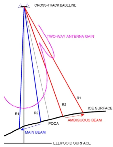
This work used intermediate level (L1b) SARIn product files in which the delay Doppler processing step has been completed to waveform data, but the processing to terrain height has not. The waveform data include the unique “point of closest approach” (POCA) followed in delay time by the sum of returns from both sides of the POCA. With a cross-track slope the POCA will be displaced from the sub-satellite track and its position and height can be calculated using the interferometric phase (Jensen, 1999). With increasing time delay beyond the POCA the composite footprint will include a region beneath the satellite with strong antenna illumina-tion and a region upslope from the POCA with weaker an-tenna illumination. This is illustrated in Fig. 1. If the upslope “range-ambiguous” region is illuminated very weakly in re-lation to the “main-beam” region, then the interferometric phase will define the cross-track look angle to the main-beam footprint and can be used with the delay time to map the po-sition and heights of the main-beam footprints. In contrast to the level 2 (L2) SARIn data product, containing only the POCA height and position, the current analysis can gener-ate an across-track swath of elevations under suitable slope conditions. This processing approach was demonstrated with ASIRAS, the ESA-developed airborne simulator for Cryosat (Hawley et al., 2009).
In Sect. 2 the problem of interferometric processing of data in which the range window includes returns from two distinct areas is addressed. The pre-launch measured antenna patterns are used in Sect. 3 to estimate the relative power in the two range-ambiguous zones. The Devon Ice Cap was selected as one of the Cryosat calibration-validation sites as it has been studied for many years (reviewed in Boon et al., 2010). Sec-tion 4 includes an outline of the swath processing steps for the L1b data collected over Devon during 2011. Two im-portant limitations of the swath processing approach are dis-cussed in Sect. 5. In Sect. 6 a product simulation approach is described that shows that the DEM produced by combining the swath processed results can be used to check and poten-tially refine the elevation data. The problems, strengths and potential of the swath processing technique are discussed in the final section.
2 Interferometry with multiple footprints
Interferometry for civilian Earth observation began in the 1980s (e.g. Zebker and Goldstein, 1986) and evolved rapidly as an important technique for terrain mapping and the mea-surement of relative terrain displacement (Rosen et al.,
1 2 3 4 5 6 7 8
Figure 1.Cryosat is oriented such that the baseline formed by the 2 receive antennas is oriented perpendicular to both the along-track direction and to the normal to the WGS84 ellipsoid. Each cross-track scan line will contain a unique estimate of the ‘point-of-closest-approach (POCA) on the ice surface, followed in delay time by the sum of returns from both sides of the POCA. With a suitable geometry the returns from the ambiguous region can be much weaker than those from the main beam underneath the satellite which allows the mapping of position and height of main beam footprints. The dashed magenta line illustrates
19 Fig. 1. Cryosat is oriented such that the baseline formed by the two receiving antennas is oriented perpendicular to both the along-track direction and to the normal to the WGS84 ellipsoid. Each cross-track scan line will contain a unique estimate of the POCA on the ice surface, followed in delay time by the sum of returns from both sides of the POCA. With a suitable geometry the returns from the ambiguous region can be much weaker than those from the main beam underneath the satellite which allows the mapping of position and height of main-beam footprints. The dashed magenta line il-lustrates diagrammatically the dB variation in cross-track two-way gain. Note that the angles have been exaggerated for clarity; the first side lobe in the pattern occurs at∼2◦from nadir and represents a two-way power level of−40 dB with respect to the power at nadir.
2000). In cross-track radar interferometry for mapping, the differential phase between the returns from two antennas is used to calculate the cross-track look angle which, together with the platform position, velocity and range, allows an ac-curate mapping of footprint height and position. However, when swath processing is used with CS L1b SARIn data we must consider the multiple range-ambiguous regions ex-plicitly. In normal SIRAL operation the left hand antenna (viewed in the direction of motion) is used for transmission and both the right and the left antennas are used for reception by the two SIRAL receivers.
L. Gray et al.: Interferometric swath processing of Cryosat data 1859
can originate from two totally separate footprints. As delay time increases beyond the POCA time one of the two range-ambiguous footprints in sloping terrain will move towards the sub-satellite track and the other will move away. We re-fer to the former as the “main” footprints and the later as the “ambiguous” footprints (Fig. 1). Note that the two parts of the composite footprint, the main and ambiguous, may be many kilometres apart but still contribute energy to the same receiver range window.
The processed receiver output connected to the left hand antennaVLi for theith fore–aft beam at zero Doppler range rLand at an arbitrary point in time (retaining only the phase term related to the radar range between the phase centres of the antennas and footprints) can be expressed as a combina-tion of the main and ambiguous components and is
VLi∝GL(θm, ϕi)
q
Amσm0(χm)exp(j krLm) (1)
+GL(θa, ϕi)
q
Aaσa0(χa)exp(j krLa).
GL(θ, ϕ)is the one-way power gain of the left hand antenna at an across-track look angle ofθ and an along-track look angle of ϕ. Am andAa are the surface areas of the main and ambiguous surface footprints defined by the pulse com-pression range resolution, the along-track delay-Doppler res-olution and the angle the beam makes with the local surface slope.σm0,a(χ )is the normalized back scattering coefficient for the main or ambiguous footprints at a surface incidence angle ofχ,j=
√
−1 andkis the wave number. The range variation in any data set is very small in relation to the satel-lite altitude so that ther5/2variation in return power (Raney, 1998) can be ignored. While the delay timing does guaran-tee that the main and ambiguous footprints are essentially at the same range, the phase terms exp(j krLm)and exp(j krLa) representing the range between the phase centre of the left antenna and the phase centres of the main and ambiguous footprints respectively are unknown and independent of one another.
Similarly the receiver output VRi connected to the right
hand antenna for one Doppler beam and range window is proportional to
VRi ∝
q
GR(θm, ϕi) GL(θm, ϕi) Amσm0(χm)exp(j krRm) (2)
+
q
GR(θa, ϕi) GL(θa, ϕi) Aaσa0(χa)exp(j krRa).
The interferogramI is formed through the look summation of the product
I=
64
X
i=1
VLi.VR∗i, (3)
where the∗symbol indicates the complex conjugate opera-tion. The phase of the interferogram then contains informa-tion on the path length differences, which can allow a geo-metric solution for the position of the footprint (as in tradi-tional cross-track interferometry). There are four terms in the
VRi.VL∗i product. Two of these, the product of the first terms
of Eqs. (1) and (2) and the product of the second terms will remain coherent as delay time increases beyond the POCA position as these terms reflect the combination of signals from the right and left antennas for the main and ambigu-ous footprints separately. The main or ambiguambigu-ous footprint size is such that when it is considered as an antenna the re-sulting “celestial footprint” subtended at the satellite is very much larger than the baseline between the two antenna phase centres and the “baseline decorrelation” condition for coher-ent interferometry is well satisfied (Rosen et al., 2000). This is not the case for the two cross terms involving a combi-nation of the first and second terms of Eqs. (1) and (2). In this case the interferogram terms are formed from a combi-nation of the main and ambiguous footprints, which are mov-ing apart as delay time increases. Consequently as the sepa-ration between the main and ambiguous footprints increases above∼10 km the cross-track celestial footprint created at the satellite will approach and eventually be less than the ac-tual baseline so that the critical baseline condition (Rosen et al., 2000) will not be satisfied. These cross terms are the reason that the coherence often decreases beyond POCA. Note that the subsequent increase in coherence is due to the fact that the differential phase for the 64 individual beams in the cross terms becomes random so that when coherently summed their contribution to the interferogram diminishes.
Consequently, when the two footprints are far enough apart the interferogramI can be approximated by the sum of the two terms from the main and ambiguous beams.
I∝
64
X
i=1
[G2(θm, ϕmi) Amσm0exp(j k1rm) (4)
+G2(θa, ϕai) Aaσa0exp(j k1ra)]
Where the two-way gainG2(θ, ϕ)=G3L/2(θ, ϕ) G1R/2(θ, ϕ) and1rm,aare the path differences from the either the main or ambiguous footprints to the two antennas. Note that the magnitude of the interferogram is now in units of power and not backscattered field amplitude. If the antenna gains illu-minating the ambiguous footprints are much less than those illuminating the main beam (<−30 dB) then the phase of the interferogram will be approximately that given by the first term in Eq. (4). With the current SIRAL transmit–receive configuration, and when the second term in Eq. (4) can be ignored, the interferogram phaseψgiven in the L1b product file can be related to the cross-track look angleθto the main footprint by
sin(θ+β)= −ψ/ kB, (5)
map the surface footprint position and height as in traditional cross-track interferometry.
3 Suppression of ambiguous returns
We estimate the relative contribution from the main and am-biguous zones as a function of cross-track slope by using prelaunch measurements of the antenna patterns (Saab Space AB, 2007). Figure 2 (top) illustrates the relationship between the circular iso-range contours and the fore Doppler beams for a locally spherical Earth model. The positions of every second Doppler beam are indicated by the dotted magenta lines extending in a grid across Fig. 2 (top). The range and angle coordinates are presented for the situation in which there is no surface slope. However, the relative positions and angles would still apply when there is a surface tilt although in this case the 0.0 point on the plot would be the position of the POCA. In “delay Doppler” processing the slant range variation for across-track footprints is compensated such that the 64 fore–aft beams for one across-track line can be regis-tered and “stacked” to reduce the speckle effect. The space-craft is accurately attitude controlled to point the peak an-tenna gain downwards perpendicular to the WGS84 ellipsoid so that, with an across-track slope, the peak antenna gain does not coincide with the POCA.
An effective two-way cross-track antenna pattern
G2-way(θ ) appropriate for interferometry was calculated using summation of the pre-launch two-dimensional patterns at the anticipated Doppler beam fore–aft angles (Wingham et al., 2006).
G2-way(θ )= i=64
X
i=1
G3L/2(θ, ϕi) G1R/2(θ, ϕi) (6)
Figure 2 (bottom) illustrates five across-track track cuts of the two-way pattern at five values of the along-track angleϕ
from 0◦ to the nominal maximum angle of∼0.76◦ as dot-ted black lines. The solid blue line represents theG2-way(θ ) sum of the 64 fore–aft two-way pattern cuts. Note that if the POCA is directly beneath the satellite then all 512 samples in range would be illuminated by the main lobe of the two-way pattern. However, with an across-track slope of 1◦, the POCA position is displaced such that the initial returns are subject to much lower two-way gain, and subsequent returns have very different antenna gains between the left and right sides of the POCA. Experience with L1b data over Devon shows that the initial returns from glacial terrain are normally still strong enough for correct operation of the tracking loop, which defines the range window, even at across-track slopes of∼1.5◦.
Figure 3 illustrates the relative power of the ambiguous beam in relation to that in the main beam for across-track terrain slopes between 0.5 and 2◦. A circular Earth was used for this simulation with the initial SARIn mode sampling
1
2
3 4 5 6 7 8 9 10 11 12 13
Figure 2 (top): The surface area illuminated by a burst of 64 pulses extends fore-aft and side-to-side of the sub-satellite point. A locally circular Earth model has been used to illustrate the relative positions of some of the circular iso-range contours and half of the 32 fore Doppler beam positions. The central (dark blue) semi-circular contours illustrate the first 9 iso-range contours after the POCA. Subsequently, the blue semi-circles indicate the positions of every 25th iso-range contour. The 512 samples in each waveform or scan line are separated in the
L1b files used in this work by 0.47 m in slant range. The cross-track footprint dimension change rapidly from the large size at POCA (~1.5 km) to ~20 m for the 400th footprint beyond
the POCA. The positions of the Doppler beams extending across-track are shown by dotted magenta lines, for clarity every second beam is shown. Both distance and angular coordinates in degrees are given for the across- and along-track dimensions with respect to the POCA.
21
Fig. 2. (Top): the surface area illuminated by a burst of 64 pulses extends fore–aft and side-to-side of the sub-satellite point. A lo-cally circular Earth model has been used to illustrate the relative positions of some of the circular iso-range contours and half of the 32 fore Doppler beam positions. The central (dark blue) semi-circular contours illustrate the first nine iso-range contours after the POCA. Subsequently, the blue semi-circles indicate the positions of every 25th iso-range contour. The 512 samples in each wave-form or scan line are separated in the L1b files used in this work by 0.47 m in slant range. The cross-track footprint dimension change rapidly from the large size at POCA (∼1.5 km) to∼20 m for the 400th footprint beyond the POCA. The positions of the Doppler beams extending across-track are shown by dotted magenta lines, for clarity every second beam is shown. Both distance and angular coordinates in degrees are given for the across- and along-track di-mensions with respect to the POCA. (Bottom): the relative two-way antenna gain is shown for cross-track cuts at five different fore an-gles corresponding to the central and the 8th, 16th, 24th and 32nd beams. These are the dashed lines while the solid blue line corre-sponds to the effective two-way patternG2-way(θ )given in Eq. (6). Note that the cross-track angle extent in Fig. 2 (bottom) is much wider than that in Fig. 2 (top).
L. Gray et al.: Interferometric swath processing of Cryosat data 1861 Figure 2 (bottom): The relative 2-way antenna gain is shown for cross-track cuts at 5 different
fore angles corresponding to the central and the 8th, 16th, 24th and 32nd beam. These are the
dashed lines while the solid blue line corresponds to the effective 2-way pattern 1
2
2way( )
G
given in Eq. (6). Note that the cross-track angle extent in Fig. 2 (bottom) is much wider than that in Fig. 2 (top).
3
4 5
6
7
8
9
10 11 12 13 14
Figure 3. Ratio of the interferogram power in the ambiguous beam to that in the main beam for cross-track slopes between 0.5° and 2.0° based on a locally spherical Earth model. The minimum in the suppression of the ambiguous power occurs when the ambiguous footprints are illuminated by the low antenna gain region between the main lobe and the first side-lobe at ~ 1.5° from nadir.
22
Fig. 3. Ratio of the interferogram power in the ambiguous beam to that in the main beam for cross-track slopes between 0.5 and 2.0◦based on a locally spherical Earth model. The minimum in the suppression of the ambiguous power occurs when the ambiguous footprints are illuminated by the low antenna gain region between the main lobe and the first side lobe at∼1.5◦from nadir.
cross-track slopes and delays from POCA that would poten-tially support swath processing.
4 Processing outline and results
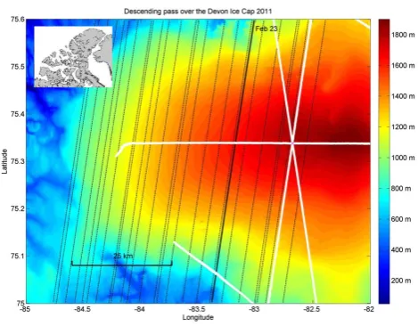
We illustrate the steps in the processing by using the de-scending pass acquired over the Devon Ice Cap on 23 Febru-ary 2011. In Fig. 4 the sub-satellite descending tracks for the period between February 2011 and January 2012 are shown as dotted black lines and the 23 February pass is shown as a solid black line. The white lines indicate the positions of the airborne laser data acquired during the 2011 CRYOVEX campaign, which have been the primary reference data for the evaluation of the Cryosat elevations.
Cryosat data are read from the ESA-provided SARIn “DBL” files (version 3.9) containing a sequence of cross-track waveform records separated by∼300 m along-track, each of which contains 512 samples of the power, coherence and phase. These values span a total range window of 240 m which will translate into a ground range swath typically up to
∼5 km. In the latest ESA data release the sampling has been increased by a factor of 2 so that the total swath window for 512 samples has been reduced to 120 m. In the L1b file each line record has already been averaged, or “multi-looked”, by summing up to 64 registered fore–aft beams. Notwithstand-ing this averagNotwithstand-ing, the interferogram output still suffers from both residual speckle and thermal noise. Phase noise has been reduced from that in the original L1b file by recreating the in-terferogram, smoothing the real and imaginary components on a line-by-line basis and extracting the phase from the
1 2 3 4 5 6 7 8 9 10
Figure 4. The western part of the Devon Ice Cap with topography illustrated in colour. The sub-satellite position of the Feb. 24th descending pass is shown as a black line and the positions of the airborne laser scanning altimeter data is shown in white. The dotted black lines indicate the sub-satellite tracks of the 25 descending passes which were used to create the DEM illustrated in Fig. 8. The position of the Devon Ice Cap in the Canadian Arctic is shown in the insert. In this figure the topography is derived from the Canadian digital elevation database merged with the CS swath processed results shown in Figure 8.
23 Fig. 4. The western part of the Devon Ice Cap with topography illustrated in colour. The sub-satellite position of the 23 February descending pass is shown as a black line and the positions of the airborne laser scanning altimeter data are shown in white. The dot-ted black lines indicate the sub-satellite tracks of the 25 descending passes which were used to create the DEM illustrated in Fig. 8. The position of the Devon Ice Cap in the Canadian Arctic is shown in the insert. In this figure the topography is derived from the Cana-dian digital elevation database merged with the CS swath processed results shown in Fig. 8.
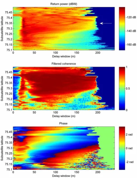
smoothed interferogram. This process effectively reduces the inherent slant range resolution from∼0.5 to∼2.5 m. The re-sulting across-track resolution then depends on the local in-cidence angle, e.g. at a local inin-cidence angle of 1◦the cross-track surface resolution is∼143 m. Note that even with the smoothing, the cross-track footprint size for swath process-ing is normally much smaller than a typical POCA footprint. The resulting power, coherence and phase are illustrated in Fig. 5 as a function of the delay window.
1
2
3 4 5
Figure 5. Illustration of the return power for the central part of the Feb. 23 pass (top), the filtered coherence (middle), and the differential phase (bottom), all as a function of the delay window expressed as a slant range distance. Note that the phase has not been unwrapped at
24
Fig. 5. Illustration of the return power for the central part of the February 23 pass (top), the filtered coherence (middle), and the dif-ferential phase (bottom), all as a function of the delay window ex-pressed as a slant range distance. Note that the phase has not been unwrapped at this stage. The white arrow in the upper image of re-turn power indicates the position of the profiles shown in Fig. 6.
The resampling from the irregularly spaced across-track sampling to a regular lat–long grid was completed in two stages: the initial processing leads to a sequence of latitude, longitude and elevation values for that part of each waveform or cross-track scan line which satisfies the coherence require-ment. Although the results are irregularly spaced, they span an almost straight line in the latitude–longitude domain. Co-efficients for a second order polynomial are obtained from a least squares fit of the latitude to the longitude values. Lati-tude and elevation data can then be interpolated at a regular sampling in longitude. For the average latitude of the Devon Ice Cap the 0.004◦sampling in longitude corresponds to a spacing of 115 m, which is larger than the normal separation of the original irregular longitude values in swath processing so that the oversampling created by the phase filtering is re-duced. The second stage is then the resampling of the eleva-tion from the irregular to regular values in latitude leading to elevations interpolated to a lat–long grid with a sampling of 0.001◦in latitude (equivalent to a spacing of∼112 m). This resampling greatly simplifies the merging of data from
differ-1
26 Fig. 6. Top: profile of the return power for the scan line at the po-sition of the white arrow in the illustration of return power in the upper part of Fig. 5. Note the leading edge is relatively weak, in-dicative of the low two-way antenna gain at the POCA cross-track angle. The strong delayed returns reflect the fact that the delayed main-beam returns have a much stronger two-way antenna gain. Second from top: profile of the smoothed coherence for the same scan line. Note that the dip in the coherence at∼30 m in the delay window corresponds to the situation when the baseline decorrela-tion affects the “cross terms” discussed in the text. The high coher-ence for the range window between∼60 and 180 m implies that the interferogram can be represented by Eq. (5) and that the returns are dominated by those from the main footprints. Third from top: the original phase from the L1b file is shown for the scan line in blue. The region of the scan line for which processing was done is shown in red. Note that the phase has been low pass filtered, the boxed region in this figure has been blown up in the bottom figure and illustrates the degree of smoothing; the red line is the unwrapped smoothed phase and the blue dots are the original values. Although it is slope dependent the sampling and resolution in the across-track direction is normally better than in the along-track direction, even with this smoothing.
L. Gray et al.: Interferometric swath processing of Cryosat data 1863
1
2
3 4 5 6
Figure 7. Illustration of the swath processed geocoded elevations for the Feb. 23rd
descending pass. The oblique white line indicates the sub-satellite track and the position of the maximum antenna gain. The 2 white arrows indicate the position of the E-W pass of the airborne ALS data which were used as a height reference.
28
Fig. 7. Illustration of the swath processed geocoded elevations for the 23 February descending pass. The oblique white line indicates the sub-satellite track and the position of the maximum antenna gain. The two white arrows indicate the position of the E–W pass of the airborne ALS data which were used as a height reference.
Figure 7 illustrates the resampled elevations as colour and shows that, in this case, results could be obtained over a cross-track distance of approximately 5 km. The results were checked against the reference airborne laser scanner (ALS) data flown over the Devon Ice Cap during the 2011 CRY-OVEX campaign. Because the laser footprint is so small (∼0.5 m2)in relation to the Cryosat swath processed foot-print (104–105m2, depending on the local incidence angle) the ALS data was used to create a reference DEM whose values were weighted averages centred on the lat–long grid used for the Cryosat geocoding. The position of the E–W ALS line is shown in Fig. 7 by the white arrows. The mean laser height minus CS swath processed height for this data set was−0.28 m and the standard deviation of the difference was 0.44 m. If the phase filtering stage was omitted the higher phase noise resulted in position errors for the footprint cen-tres and the standard deviation of the difference increased to 0.74 m. In both cases∼100 height differences were used.
Results from 24 ascending and 25 descending passes were combined separately to create two DEMs. These data were acquired throughout the period from February 2011 to Jan-uary 2012, usually two or three acquisitions per month for both ascending and descending passes. The DEM illustrated in Fig. 8 was created from a combination of the results from the 25 descending passes and Fig. 9 illustrates the compari-son between the CS and airborne laser altimeter derived ref-erence data. The E–W elevation profile at 73.339 N is shown
1
2 3 4 5 6
Figure 8. Results from 25 descending passes have been combined to create a DEM of the western slopes of the Devon Ice Cap. Colour has been used to indicate height in meters. The uneven edges of the DEM at the north and south edges are due to the relatively large along-track slope and the resulting poor solution often indicated by lower data coherence and higher phase noise.
29
Fig. 8. Results from 25 descending passes have been combined to create a DEM of the western slopes of the Devon Ice Cap. Colour has been used to indicate height in metres. The uneven edges of the DEM at the north and south edges are due to the relatively large along-track slope and the resulting poor solution often indicated by lower data coherence and higher phase noise.
in the upper plot and the histogram of height differences be-tween the CS and ALS data is illustrated in the middle. The mean difference is 0.49 m and the standard deviation of the height differences is 0.75 m. The lower plot in Fig. 10 illus-trates the E–W slope (approximately across-track) and shows that the western slopes of the Devon Ice Cap do match those predicted by Fig. 3 as being appropriate for swath processing.
5 Impact of interferometric phase and roll angle errors
on swath processed height errors
1 2 3 4
Figure 9. The upper plot illustrates the E-W elevation at 73.339 N for both the Cryosat DEM data and the ALS laser heights. The middle plot illustrates the histogram of the height differences and the lower plot shows the E-W slope derived from the Cryosat results.
30 Fig. 9. The upper plot illustrates the E–W elevation at 73.339 N for both the Cryosat DEM data and the ALS laser heights. The middle plot illustrates the histogram of the height differences and the lower plot shows the E–W slope derived from the Cryosat results.
resulting bias in height would be∼1.3 m. In summary, the first order error in derived heightεhdepends on the error in the cross-track off-nadir angle and the local incidence angle
χlocal, and is given by
εh= εph/[kB] +εrollr χlocal. (7) In Eq. (7) we assume that the off-nadir angles are small enough that sinθ=θand that any error in rangeris negligi-ble. The phase errorεphcan be due to phase noise, phase cal-ibration drift and also through the assumption that the inter-ferogram phase reflects just the main footprints when in fact there may be a small contribution from the ambiguous re-gion. The roll angle errorεrollis not constant and may reflect the changing thermal environment (Galin et al., 2013). As
χlocalis essentially zero for the POCA this equation implies that swath processing will not achieve the height accuracies possible with the standard geophysical L2 POCA height es-timates. This is certainly true for the range of cross-track an-gles for which the SARIn mode was expected to work (nomi-nally <∼0.6◦, note the phase will “wrap” at an off-nadir an-gle of∼0.54◦complicating the operational algorithm). How-ever, our experience with the L2 results over Devon, is that when either the across- or along-track angle exceeds∼0.5◦
1
2 3 4 5 6
7
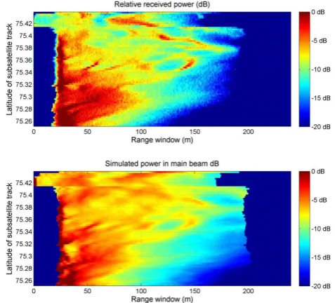
Figure 10. Comparison of the relative received power (upper image) with the simulated power for the main beam (lower image) for the Feb 23 descending pass data. In both cases the dynamic range from blue to red is 20 dB and in each case the dB scale is with respect to the maximum value. The simulation is based on the footprint size, a near-nadir backscatter model and the two-way antenna gain pattern given by Eqn. 6.
31 Fig. 10. Comparison of the relative received power (upper image)
with the simulated power for the main beam (lower image) for the 23 February descending pass data. In both cases the dynamic range from blue to red is 20 dB and in each case the dB scale is with respect to the maximum value. The simulation is based on the foot-print size, a near-nadir backscatter model and the two-way antenna gain pattern given by Eq. (6).
the leading edge of the POCA return is quite variable and the “retracker” required to identify the POCA position and inter-polate the POCA phase may not generate reliable results. In essence, the operational SARIn mode was not designed for larger off-nadir angles. This shows that swath processing can complement the L2 results by providing heights in an across-track off-nadir angle regime, which is outside the range for which we expect good L2 POCA results.
L. Gray et al.: Interferometric swath processing of Cryosat data 1865
any correction, the average difference between the resulting Cryosat DEM and the reference data increased to∼2.6 m but the standard deviation about the mean only increased from 0.75 to 0.83 m. This area is still under active investigation.
The impact of an unknown ambiguous zone contribution is not easy to anticipate a priori but the use of data simulation using the derived DEM does help evaluate the results; this is discussed further in the section below. The worst case height error occurs when the phase of the ambiguous zone contri-bution is some multiple ofπ/2 with respect to the phase of the main-beam contribution. If the ambiguous power is 30 dB below that in the main beam then the worst case error in the look angle is∼9.5 10−5radians leading to a height error of 38 cm if the local incidence angle in the main beam is 0.5◦.
6 Data simulation
Cross-track profiles of elevation as a function of position can be estimated from the CS generated DEMs for each scan line. By using the satellite position and timing information this al-lows the estimation of look angle, cross-track slope, local in-cidence angle and footprint size for each of the cross-track footprints. Note that this can be done for both the “main” and “ambiguous” beams separately. Also, the relative power in the main and ambiguous beams can be estimated using the footprint size, the local incidence angle and the antenna gain patterns. The relative power for the 23 February data is illustrated in the upper panel of Fig. 10 and the simulated power for the main beam is illustrated in the lower panel. This was based on the size of the footprint in the main beam and a relative backscatter model linear in local incidence an-gle (−2.5 dB times the local incidence in degrees) and clearly captures the main features of the actual data. In the same way, the relative received power in the range-ambiguous beam can be compared to that in the main beam directly beneath the satellite. This shows that for much of the received swath the contribution of the upslope range-ambiguous region is very small (−30 to−40 dB with respect to the main beam). Also, with the knowledge of the look angles it is possible to esti-mate the phase as well as the magnitude of the contribution from the ambiguous region so that regions with potentially significant errors can be removed. However, with the cross-track slopes on the western flank of the Devon Ice Cap, the minimum coherence criteria used already eliminates much of the areas affected by the ambiguous regions upslope. A re-examination of the processed data shows that while the simulation approach does improve results through the elimi-nation of some poor regions the problem of small bias errors can remain.
7 Discussion and conclusions
The increased data volume possible with swath processing of Cryosat SARIn L1b data over sloping glacial ice allows the creation of DEMs where previously radar altimetry pro-vided only a sparsely sampled along-track elevation profile often with some uncertainty as to the position of the footprint (see e.g. Hurkmans et al., 2012). Even at latitude∼75◦N the available data from one year over the Devon Ice Cap was suf-ficient to allow the creation of DEMs from both ascending and descending passes. At higher latitudes the sub-satellite tracks converge and the task becomes easier.
However, there are problems that do not exist with the con-ventional processing to the L2 SARIn products. Firstly, the time-delayed footprints beyond POCA contain contributions from at least two footprints and useful results can only be generated when the returns from one contiguous footprint are much stronger (>∼30 dB) than any other footprint in the same time-delay window. This restricts the method to areas with an average cross-track slope of∼0.5 to∼2◦. Secondly, swath processing places stringent requirements on the base-line roll angle and phase calibration, which are difficult to satisfy. In particular, the uncertainty in the baseline roll an-gle will lead to biased height errors. Careful comparison of the CS DEM results with our various surface elevation data shows that spatially varying bias errors of order 1 m can exist. Further, we find that there appears to be a bias again of order 1 m between the DEM derived from the descending passes and that derived from the ascending passes. The reason for this difference remains uncertain. However, one advantage of swath mode processing is that the complexity associated with interpolating the surface return position (the “retracker”) is avoided.
Once a DEM of the area has been completed it is possible to use the simulation approach to estimate the contribution from the various footprints and to further refine the results through the elimination of any data, which may have signifi-cant errors. Our results over Devon also show that results are worse when there is an average along-track slope >∼0.5◦, or when there is significant topographic variation. For exam-ple it was much more difficult to obtain useful results on the eastern flank of the Devon Ice Cap which has a much more varied topography.
mapping of the slope in the direction of movement (related to the driving stress) and also the mapping of surface elevation “dips” in ice streams and glaciers such as the elevation results derived from 19 Cryosat descending passes for the subglacial Lake Mercer (SLM) and shown in Gray et al. (2013). Peri-odic filling and draining of SLM and many other subglacial lakes was documented by Fricker et al. (2007) and Smith et al. (2009) with ICESat data after the initial observation of the associated vertical surface movement through 3-D InSAR work (Gray et al., 2005). The increased data volume possible with CS swath processing combined with the improved spa-tial resolution will help in mapping the surface subsidence or inflation associated with the periodic filling or draining of subglacial lakes. In this regard McMillan et al. (2013) have already used Cryosat data to measure the ice surface uplift subsequent to the drainage of the CookE2 subglacial lake originally identified by Smith et al. (2009). Although they used the Cryosat level 2 elevation results, the improved resolution and ability to map the cross-track position of the footprint helped make this possible.
While these new results on DEM creation from Cryosat L1b SARIn data are encouraging, further work is required to better refine and exploit this potentially valuable data source. In the current work, airborne laser data was used to refine results, this is clearly not generally possible. However, other approaches are possible; low resolution DEMs for Antarctica or Greenland (e.g. Bamber et al., 2009) could be used as an initial input for simulation and then refinement of swath pro-cessing results. Also for appropriate cross-track slopes the POCA estimates from either the ESA L2 or L1b files could be used as reference data to help refine the baseline roll an-gle or the potential contribution from the range-ambiguous zone in swath processing. Work is underway to explore these options. The ultimate height accuracy possible with swath mode Cryosat processing remains to be determined but the Devon results imply that height errors with a standard devia-tion of less than 1m are possible, although there can be bias errors of order 1 m.
Acknowledgements. ESA provided the Cryosat data and supported
the Devon Ice Cap cal/val experiment through the CRYOVEX overflights. The Technical University of Denmark team, led by Rene Forsberg, operated the CRYOVEX instruments and processed the airborne laser scanner (ALS) altimeter data used as the reference data. Mike Demuth, GSC, initially led the Canadian Cryosat-related work on the Devon Ice Cap, his contributions are gratefully acknowledged. D. Wingham, the driving force behind Cryosat and formerly Principal Scientist, provided useful input and encouragement for the initial stages of this work. Natural Resources Canada (D. Burgess, ESS Contribution number 20130133), NSERC (L. Copland), NASA (grant NNX10AG22G to R. Hawley), the German Ministry of Economics and Technology (Grant 50EE1008 to V. Helm), and the Canadian Space Agency (GRIP grant to D. Burgess) have supported this work.
Edited by: R. Kwok
References
Bamber, J. L., Gomez-Dans, J. L., and Griggs, J. A.: A new 1 km digital elevation model of the Antarctic derived from combined satellite radar and laser data – Part 1: Data and methods, The Cryosphere, 3, 101–111, doi:10.5194/tc-3-101-2009, 2009. Boon, S., Burgess, D., Koerner, R., and Sharp, M.: Forty seven years
of research on the Devon Ice Cap, Arctic Canada. Arctic, 63, 13– 29, 2010.
Fricker, H. A., Scambos, T., Bindschadler, R., and Padman, L.: An active subglacial water system in West Antarctica mapped from space, Science, 315, 1544–1548, 2007.
Gardelle, J., Berthier, E., and Arnaud, Y.: Slight mass gain of Karakoram glaciers in the early twenty-first century, Nat. Geosci., 5, 322–325, 2012.
Galin, N., Wingham, D. J., Cullen, R., Fornari, M., Smith, W. H. F., and Abdall, S.: Calibration of the Cryosat Interferometer and Measurement of Across-track Ocean Slope, IEEE T. Geosci. Re-mote., 51, 57–72, 2013.
Gray, L., Joughin, I., Tulaczyk, S., Spikes, V., Bindschadler, B., and Jezek, K.: Evidence for subglacial water transport in the West Antarctic Ice Sheet through 3-dimensional satel-lite radar interferometry, Geophys. Res. Lett., 32, L03501, doi:10.1029/2004GL021387 2005.
Gray, L., Burgess, D., Copland, L., Galin, N., and Cullen, R.: Using the Cryosat Interferometric swath mode for glacial ice topogra-phy: Proceedings of the 2012 ESA EO4Cryosphere Conference, ESA Special Publications SP 712, May 2013.
Hawley, R. L., Shepherd, A., Cullen, R., and Wingham, D. J.: Ice-sheet elevations from across-track processing of airborne in-terferometric radar altimetry, Geophys. Res. Lett., 36, L25501, doi:10.1029/2009GL040416, 2009.
Hurkmans, R. T. W. L., Bamber, J. L., and Griggs, J. A.: Brief com-munication “Importance of slope-induced error correction in vol-ume change estimates from radar altimetry”, The Cryosphere, 6, 447–451, doi:10.5194/tc-6-447-2012, 2012.
Jensen, J. R.: Angle measurement with a Phase-Monopulse radar altimeter, IEEE Trans. Antennas Propag., 47, 715–724, 1999. McMillan, M., Corr, H., Shepherd, A., Ridout, A., Laxon, S., and
Cullen, R.: Three-dimensional mapping by Cryosat-2 of sub-glacial lake volume changes, Geophys. Res. Lett., 40, 4321– 4327, 2013.
Parrinello, T., Mardle, N., Bouzinac, C., Badessi, S., Frommknecht, B., Davidson, M., Hoyos, B., and Fornari, M.: CryoSat: ESA’s Ice Explorer Mission: Two Years in Operations: Status and Achievements, Abstract book: Third Cryosat Users Workshop, Dresden, Germany, 2013.
Raney, R. K.: The delay/Doppler radar altimeter, IEEE T. Geosci. Remote, 36, 1578–1588, 1998.
Rosen, P., Hensley, S., Joughin, I., Li, F., Madsen, S., Rodriguez, E., and Goldstein, R.: Synthetic Aperture Radar Interferometry, Proc. IEEE, 88, 333–382, 2000.
L. Gray et al.: Interferometric swath processing of Cryosat data 1867
A., van Angelen, J., van der Berg, W., van den Broeke, M., Vaughan, D., Velicogna, I., Wahr, J., Whitehouse, P., Wingham, D., Donghui, Y., Young, D., and Zwally, J.: A reconciled estimate of ice-sheet mass balance, Science, 338, 1183–1189, 2012. Smith, B., Fricker, H., Joughin, I., and Tulaczyk, S.: An inventory of
active subglacial lakes in Antarctica detected by ICESat (2003– 2008), J. Glaciol., 55, 573–595, 2009.
Wingham, D. J., Phalippou, L., Mavrocordatos, C., and Wallis, D.: The mean echo and echo cross-product from a beam forming, interferometric altimeter and their application to elevation mea-surement, IEEE T. Geosci. Remote, 42, 2305–2323, 2004.
Wingham, D., Francis, C., Baker, S., Bouzinac, C., Brockley, D., Cullen, R., de Chateau-Thierry, P., Laxon, S., Mallow, U., Mavrocordatos, C., Phalippou, L., Ratier, G., Rey, L., Rostan, F., Viau, P., and Wallis, D.: Cryosat: A Mission to determine the Fluctuations in Earth’s Land and Marine Ice Fields, Adv. Space Res., 37, 841–871, 2006.
Zebker, H. and Goldstein, R.: Topographic mapping from inter-ferometric SAR observations, J. Geophys. Res., 91, 4993–4999, 1986.