The Cryosphere, 5, 727–740, 2011 www.the-cryosphere.net/5/727/2011/ doi:10.5194/tc-5-727-2011
© Author(s) 2011. CC Attribution 3.0 License.
The Cryosphere
The Potsdam Parallel Ice Sheet Model (PISM-PIK) – Part 2:
Dynamic equilibrium simulation of the Antarctic ice sheet
M. A. Martin1,2, R. Winkelmann1,2, M. Haseloff1,3, T. Albrecht1,2, E. Bueler4,5, C. Khroulev5, and A. Levermann1,2
1Earth System Analysis, Potsdam Institute for Climate Impact Research, Potsdam, Germany 2Institute of Physics, Potsdam University, Potsdam, Germany
3Department of Physics, Humboldt-University, Berlin, Germany
4Department of Mathematics and Statistics, University of Alaska, Fairbanks, USA 5Geophysical Institute, University of Alaska, Fairbanks, USA
Received: 15 July 2010 – Published in The Cryosphere Discuss.: 18 August 2010 Revised: 5 July 2011 – Accepted: 22 August 2011 – Published: 14 September 2011
Abstract. We present a dynamic equilibrium simulation of the ice sheet-shelf system on Antarctica with the Pots-dam Parallel Ice Sheet Model (PISM-PIK). The simulation is initialized with present-day conditions for bed topogra-phy and ice thickness and then run to steady state with con-stant present-day surface mass balance. Surface tempera-ture and sub-shelf basal melt distribution are parameterized. Grounding lines and calving fronts are free to evolve, and their modeled equilibrium state is compared to observational data. A physically-motivated calving law based on horizon-tal spreading rates allows for realistic calving fronts for var-ious types of shelves. Steady-state dynamics including sur-face velocity and ice flux are analyzed for whole Antarctica and the Ronne-Filchner and Ross ice shelf areas in particu-lar. The results show that the different flow regimes in sheet and shelves, and the transition zone between them, are cap-tured reasonably well, supporting the approach of superpo-sition of SIA and SSA for the representation of fast motion of grounded ice. This approach also leads to a natural emer-gence of sliding-dominated flow in stream-like features in this new 3-D marine ice sheet model.
1 Introduction
One of the most severe shortcomings of the Fourth Assess-ment Report (AR4) of the IntergovernAssess-mental Panel on Cli-mate Change (IPCC) was the lack of a process-based
assess-Correspondence to: A. Levermann ([email protected])
ment of future sea-level rise for the 21st century and be-yond. While the direct effect of oceanic warming and re-lated thermal expansion are captured with some uncertainty by state-of-the-art climate models, modeling studies for fast processes in land ice continue to be sparse. Observations, however, support the importance of modeling these ice flow processes. On the Antarctic Peninsula, for example, an ac-celeration of ice flow across the grounding line has been ob-served in response to ice-shelf disintegration (e.g., Pritchard et al., 2009; Rott et al., 2011). The fast ice flow regimes in the vicinity of the grounding line as well as ice-shelf dynamics constitute two of the largest challenges in ice sheet modeling. Here we present a simulation for the Antarctic sheet-shelf system with the Potsdam Parallel Ice Sheet Model (PISM-PIK) with a special focus on both ice shelf dynamics and the transition zone between grounded and floating ice.
margin, a parameterization for subgrid-scale motion of ice-shelf fronts (Albrecht et al., 2011) and a new calving-rate law which is presented in Levermann et al. (2011).
In this paper we first describe the set-up for a dynamic equilibrium simulation for Antarctica in Sect. 2. Section 3 presents the performance of PISM-PIK under present-day conditions in this simulation and summarizes and discusses it in comparison with observations. A conclusion is given in Sect. 4.
2 Model setup for the dynamic equilibrium simulation
For our dynamic equilibrium simulation the following model setup is used: the model domain is discretized on a 301×301 horizontal grid with 19.98 km spacing. The vertical grid has 51 levels within a domain extending 5000 m above the bed elevation. The vertical spacing ranges from 26.5 m in the lowest layer to 173.5 m spacing at the surface of the thick-est ice. The temperature is stored on this unequally-spaced grid, but the equation of conservation of energy is solved on a vertical grid with uniform spacing of 26 m. A thin bedrock layer of 265 m with 26.5 m spacing was used, following the reasons given in Bueler and Brown (2009).
The input fields for topography and initial ice thickness are regridded from the present-day ALBMAP v1 data (Le Brocq et al., 2010) available on the SeaRISE (2011) project web-site. These data update the earlier BEDMAP (Lythe et al., 2001). Surface mass balance is adopted from Van de Berg et al. (2006), and geothermal flux is based on the model of Shapiro amd Ritzwoller (2004). Throughout the equilibrium simulation surface mass balance, geothermal flux and bed to-pography are held fixed. Notation for this paper is in Ta-ble A1.
Similar to Huybrechts (1993) and Pollard and Deconto (2009), the surface temperature field is parameterized as a function of latitude and surface elevation:
Ts=273.15+30−0.0075h−0.6878|8| (1)
with latitude|8|in◦S; temperature is given in Kelvin. This parameterization reproduces the observed temperatures for the present-day surface elevation (Comiso, 2000; Van den Broeke, 2008), particularly on the ice shelves.
This surface temperature field serves as a Dirichlet bound-ary condition to the equation of conservation of energy (Eq. 3 in Winkelmann et al., 2011) which governs thermodynamics within the ice body. This has not changed compared to PISM and is described in detail in Bueler and Brown (2009); Bueler et al. (2007).
At the base of the ice shelf we provide boundary condi-tions both for the temperature field as well as a sink/source term for the mass continuity equation (Eq. 1 in Winkelmann et al., 2011) which incorporates basal melting and refreez-ing. For the temperature evolution within the ice we define
the boundary as ice which is at pressure melting tempera-ture. Hence the pressure-melting temperatureTpmis applied
as a Dirichlet boundary condition to the conservation of en-ergy equation:
Tpm=273.15+βCCzb (2)
withzbas the elevation (generally negative) of the base of the
ice shelf and with Clausius-Clapeyron gradientβCC.
Con-cerning the basal melting and refreezing a warm and saline ocean is the determining factor: a mass fluxSfrom shelf to ocean
S=Qheat/(Liρi) (3)
whereLi is the latent heat capacity of ice andρi ice
den-sity, is computed from a heat fluxQheat. This heat flux is
determined following Beckmann and Goosse (2003) using a virtual temperatureTf, which is the freezing temperature of
ocean water at the depthzbbelow the ice shelf
Tf=273.15+0.0939−0.057So+7.64×10⁻⁴zb. (4)
HereSois the salinity of the ocean with a value of 35 psu.
The transition from the base of the shelf with a salinity close to zero (Oerter et al., 1992) to the ocean water of full salinity occurs in the oceanic mixed layer which we cannot resolve in our approach. The resulting heat flux between ocean and ice, representing the melting effect of the ocean through both temperature and salt, is computed from
Qheat=ρocpoγTFmelt(To−Tf) , (5)
with ρo density of ocean water and cpo specific heat
ca-pacity of the ocean mixed layer. For the present simula-tionTois set to a constant value of−1.7◦C (see Table A1),
based on the NCEP reanalysis value for the Ross Ice Shelf given in Beckmann and Goosse (2003). HereγTis the
ther-mal exchange velocity andFmelt a model parameter. While
we adopt a value ofγ=10−4(Holland and Jenkins, 1999; Hellmer and Olbers, 1989) the tuning process showed that the introduction of the model parameterFmelt, with a value of
Fmelt=5×10⁻³was necessary in order to match the present
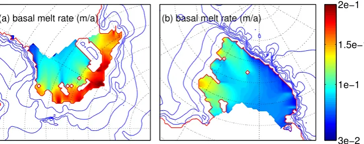
position of the grounding line especially in West Antarctica. This results in a low magnitude of the melt rate shown in Fig. 1. The spatial pattern of subshelf melt rates however depends on the shelf bottom temperature which is closely re-lated to the shelf thickness, which is supported by Beckmann and Goosse (2003).
As detailed in Winkelmann et al. (2011), Sect. 2.2, ice ve-locities are calculated in PISM-PIK as the sum of the SIA velocities and the SSA velocities with basal resistance that are computed everywhere in the grounded ice. In fact, for grounded ice the SSA velocity is interpreted as the basal sliding velocityvb(Bueler and Brown, 2009). This provides
M. A. Martin et al.: PISM-PIK – Part 2 729
Table 2. Comparison with observations of key quantities in the PISM-PIK dynamical equilibrium simulation
(Lytheet al., 2001; Le Brocqet al., 2010). The column labeled “difference” is the amount by which the model
result exceeds observations.
Quantity Observations PISM-PIK Difference
Total ice volume 256×1014m3 258×1014m3 +0.8%
Grounded ice volume 249×1014m3 254×1014m3 +2.0%
Total ice area 137×1011m2 136×1011m2 −0.7%
Grounded ice area 123×1011m2 125×1011m2 +1.6%
Floating ice area 143×1010m2 111×1010m2 −22.4%
Ice front type: marine 28% 54% –
Ice front type: cliff 25% 23% –
Ice front type: shelf 47% 23% –
(a) basal melt rate (m/a) (b) basal melt rate (m/a)
3e−2 1e−1 1.5e−1 2e−1
Fig. 1: Basal melt rate for(a)Ronne-Filchner and(b)Ross Ice Shelves, as given by Eq. (3). The
parameterization used here leads to melt rates which depend on the shelf thickness and are highest
near the grounding lines (red). Blue lines are contours of surface elevation.
18
Fig. 1. Basal melt rate for (a) Ronne-Filchner and (b) Ross Ice Shelves, as given by Eq. (3). The parameterization used here leads to melt rates which depend on the shelf thickness and are highest near the grounding lines (red). Blue lines are contours of surface elevation.
where noteworthy sliding occurs, and from rapidly-sliding ice across the grounding line to an ice shelf. The reasoning supporting this approach and its placement within the family of shallow and hybrid models is given in the description pa-per of PISM-PIK, Winkelmann et al. (2011). In contrast to PISM we do not use a weighting function to combine the two velocity contributions, but simply add them. Features that we call “streams” in the context of this simulation are defined di-agnostically as regions where SSA (i.e., basal) velocitiesvb
are larger than SIA velocities,
vb>v¯−vb (6)
withv¯ the vertical average of the full velocityvSIA+vSSA.
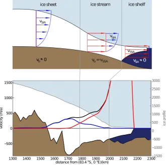
Figure 2 shows the velocity patterns emerging from the superposition of SIA and SSA velocities for an example cut through the sheet-shelf transition zone of the Lambert Glacier and the Amery Ice Shelf in the simulation. This ex-ample illustrates how the two velocity contributions super-sede each other in the sheet and in the ice shelf except in a transition region in the upper part of a stream-like flow pat-tern. The onset of this transition region can be found where the SSA velocity rises above the SIA velocity on grounded ice, i.e., where the red curve crosses the blue curve in Fig. 2. This observed smooth transition from quasi no-slip in the interior of the ice sheet to sliding is a result of the solution of the free boundary problem analyzed in Schoof (2006b), in which both locations of sliding and the sliding velocity are solved-for simultaneously as parts of the whole ice sheet application of the SSA stress balance. This whole ice sheet SSA computation is done at every time step of the dynamic equilibrium model. In many models the onset of sliding frequently arises from a transition from cold ice to ice at pressure-melting-temperature at the base, but in PISM-PIK no sliding onset is imposed there or elsewhere. Rather, the basal material yield stressτcevolves according to the
Mohr-Coulomb equation, Eq. (9), the driving stress evolves accord-ing to the mass continuity equation (Eq. 1 in Part 1), and the
solution of the SSA itself determines whether the (regular-ized) plastic basal material fails and sliding occurs. Since the basal yield stress is a continuous function of ice thickness and topography in our parameterization (Eqs. 9–12) we ensure a smooth onset of sliding without prescribing any internal boundary conditions. The other transition, from grounded to floating ice, works also without imposing any boundary con-dition. The grounded/floating-mask is determined in every time step from the flotation criterion:
b(x,y)= −ρi ρo
H (x,y) . (7)
Hence migration of the grounding line is – via the evolution of the ice thickness – determined by the velocities computed from the stress balance. Since, like in other SSA-models used for floating and grounded ice, velocities are computed non-locally and simultaneously for the shelf and as a sliding velocity for the sheet, they provide a natural way to take into account buttressing effects, and stress transmission across the grounding line is guaranteed. We believe that this provides a good alternative to boundary conditions being imposed at the grounding line in order to combine shelf flow and defor-mational flow inland in a large scale model.
Basal friction within the SSA equations, which is crucial for the magnitude of the computed sliding velocities, is cal-culated based on a model for plastic till (Schoof, 2006a) τbi= −τc
vi
v2
x+vy2
1/2, (8)
as described in Winkelmann et al. (2011). The basal yield stressτcis given by the Mohr-Coulomb model for saturated
till with zero cohesion (Paterson, 1994)
τc=tanφ (ρigH−pw) . (9)
1300 1400 1500 1600 1700 1800 1900 2000 2100 2200 2300 −500 0 500 1000 1500
distance from (83.4 S, 0 E)(km)
v e lo c it y ( m /a ) −1500 −1000 −500 0 500 1000 1500 2000 2500 3000 ic e p ro fi le ° °
ice sheet ice stream ice shelf
SIA
v
SIA
v
b v = vb SSA v SIA 0
SSA
v
∼∼
∼
v 0
∼
Fig. 2: Superposition of SIA and SSA velocities. Upper panel: a schematic diagram of an ice profile
showing the different flow regimes in PISM-PIK. Repeats Fig. 1 from Winkelmann
et al.
(n.d.).
Lower panel: an example cut through the sheet-stream-shelf transition of the Lambert Glacier and
Amery Ice Shelf in the simulation. The location is shown by the green line in Fig. 8. The onset of
an ice stream is defined diagnostically to be where the basal sliding velocity
v
b(red curve) exceeds
the SIA velocity
v
SIA(blue curve). The model output velocity
v
=
v
b+
v
SIAis shown in black.
19
Fig. 2. Superposition of SIA and SSA velocities. Upper panel: a schematic diagram of an ice profile showing the different flow regimes in PISM-PIK. Repeats Fig. 1 from Winkelmann et al. (2011). Lower panel: an example cut through the sheet-stream-shelf transition of the Lambert Glacier and Amery Ice Shelf in the simulation. The location is shown by the green line in Fig. 8. The onset of an ice stream is defined diagnostically to be where the basal sliding velocityvb(red curve) exceeds the SIA velocityvSIA(blue curve). The model output
velocityv=vb+vSIAis shown in black.
is only valid where sliding is occurring. Because the basal stress is computed by a regularized plastic law (Bueler and Brown, 2009, Eq. 27), however, at stresses lower than the yield stress there is a very small amount of sliding on the or-der of 10 cm a−1or less. Comparison to an exact solution of
the perfectly-plastic model shows that this regularization in-deed has only a small effect (Bueler and Brown, 2009). The designation of “non-sliding-ice” is therefore applied to the vast regions in the interior of the ice sheet with such negligi-bly small SSA velocities, recognizing that they would have exactly zero basal sliding in a perfectly-plastic model. For our simulation of Antarctica, the friction angleφ (Clarke, 2005) is parameterized with bed elevation as
φ (x,y)=
5◦, b(x,y)≤ −1000,
5◦+15◦1+b(x,y)
1000
, −1000<b(x,y)<0,
20◦, 0≤b(x,y)
(10)
The pore water pressure
pw=0.96ρigH λ (11)
is limited to a maximum of 96 % of the overburden pressure ρigH for maximal λ, i.e., for ice resting on bedrock at or
below sea level. The scaling parameterλ, given by
λ(x,y)=
1, b(x,y)−zsl≤0,
1−b(x,y)−zsl
1000
0< b(x,y)−zsl<1000,
0, 1000≤b(x,y)−zsl,
(12)
ranges, depending on sea level zsl and bed elevation, from
M. A. Martin et al.: PISM-PIK – Part 2 731 parameterization, exactly like the thermodynamical model,
essentially gives uniformly full water content (λ=1), lead-ing to low basal resistance there allowlead-ing for slip or fast sliding. Thus effective pressure varies linearly between 4 % of overburden pressure in marine areas and full overburden where the bed exceeds 1000 m a.s.l. The parameterization ensures a continuous transition to a quasi-non-slip regime in regions higher up, where the basal resistance is higher and sliding gets less and less pronounced, until it is negligibly small in the interior of the ice sheet, which can be regarded as frozen to the bedrock (see Figs. 3 and 2). The low basal resistance in marine areas is crucial for the development of fast flow and stream-like flow patterns as illustrated, for ex-ample, in Fig. 11. More data or also a new thermodynami-cal model providing a more detailed picture about the con-ditions at the base of the ice would be needed to precisely model the locations and velocities of streams in Antarctica. Inverse modeling (e.g., Macayeal, 1992; MacAyeal, 1993; Maxwell et al., 2008; Raymond and Gudmundsson, 2009; Joughin et al., 2009; Arthern and Gudmundsson, 2010; Gold-berg and Sergienko, 2011) would improve the parameteriza-tion of basal fricparameteriza-tion, but basal fricparameteriza-tion is not the only control mechanism for the structure of what we identify as streams in this simulation. This is because they arise from the simulta-neous solution of the thermomechanically-coupled SSA and SIA equations. The role of longitudinal stresses is critically important in generating convergence to credible continuum results, see Bueler and Brown (2009). Also the horizontal resolution is crucial in resolving ice streams, as the dimen-sion of actual ice streams often is at or below the≈20 km resolution used in this simulation.
When aiming at modeling different flow regimes, the isotropic (Glen) flow law used here (Winkelmann et al., 2011, Eqs. 4–5) might not be the best choice. Ma et al. (2010) suggest that velocities in the grounded part of an ice sheet are often underestimated by models using such isotropic laws, while they are overestimated in ice shelves. In applying PISM-PIK to the Antarctic sheet-shelf system we adjust for un-modeled anisotropy, and also for other uncertainties re-lating to unobserved variations in viscosity and basal resis-tance, by using different enhancement factors for the SIA (ESIA) and the SSA (ESSA). Note ESIA>1 and ESSA<1;
see Table A1 for values. This difference in quality for the two enhancement factors is justified by the fact that under compression the fabric of ice becomes axisymmetric and eas-ier to shear than isotropic ice, whereas under tension girdle-type fabrics evolve and make the ice stiffer (Ma et al., 2010). In PISM-PIK we use a uniform enhancement factor for the SSA, but, because the SSA velocity is interpreted as the slid-ing velocity for grounded ice, the effective flow enhance-ment arising from the superposition decreases for ice flowing through the transition from sheet to shelf; compare Fig. 2.
At all types of ice margins the SSA stress balance is sub-ject to a physically motivated stress boundary condition (for details see Sect. 2.4 in Winkelmann et al., 2011). For ice
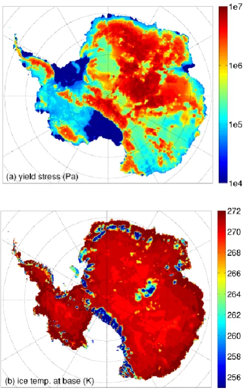
Fig. 3. (a) Map of yield stressτc, following Eqs. (9–12). (b) Tem-perature at the base of grounded ice.
shelves, a subgrid-interpolation of the calving front enables continuous advance and retreat and also ensures a steep front, which is necessary for a proper evaluation of the stresses there (see Albrecht et al., 2011). Advance of the calving front naturally happens through mass transport governed by the continuity scheme, while retreat is governed by a new physically-motivated calving law.
In fact, following Levermann et al. (2011), calving occurs in regions of divergent flow where both eigenvalues˙± of the horizontal strain rate tensor are positive. In such cases we define the calving rate to be
C=Kdet(˙)=K˙+˙− for ˙±>0 (13) withK>0 being a proportionality constant. This calving law allows for realistic calving fronts for various types of shelves, e.g., relatively thin ones like Larsen C with ice thicknesses Hc of about 170–220 m at the calving front as well as for
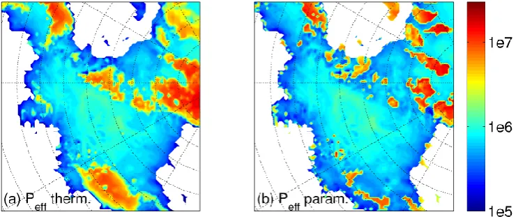
Fig. 4. Effective pressure with pore water pressure according to Eq. (11) with (a)λthermodynamically computed as in Bueler and Brown (2009) and (b) parameterized according to Eq. (12).
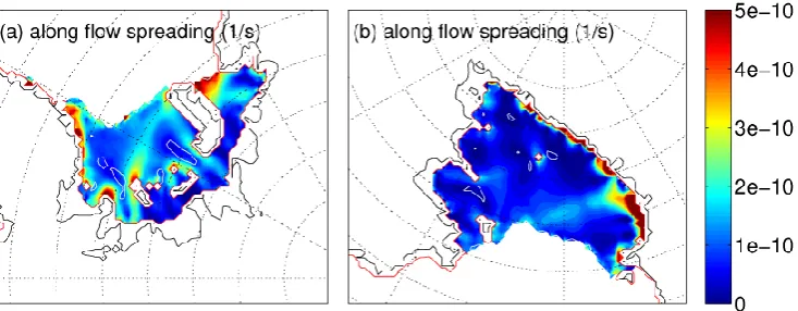
new calving law ensures that shelf ice is cut off at the mouth of bays, like the Ross bay, for example. In Fig. 5 the along-flow eigenvalue˙+for our simulations is illustrated together with the zero lines for the across-flow eigenvalue˙−. In most parts, this second eigenvalue is negative, indicating compres-sion within the shelf. Regions where˙−is positive – indicat-ing expansion in the transversal direction – are critical in the sense that once a calving front retreats back to such a position a new stable calving front position is established. Conver-gence of ice flow can be produced by pinning points like ice rises, islands or predominant coast features, which stabilize the calving front.
3 Performance in equilibrium simulation
PISM-PIK as described above in Sect. 2 was applied to the Antarctic ice-sheet-shelf system in a dynamic equilibrium simulation using time-invariant input data. After initializa-tion with presently-observed fields the model reached an equilibrium with 258×1014m3ice volume compared to the 256×1014m3deduced from the ALBMAP data set. The first part of the spin up procedure consisted of a 200 000 yr model run with fixed geometry and non-evolving surface such that the three-dimensional temperature field within the ice body could evolve to equilibrium according to the conservation of energy equation. Afterwards the dynamic equilibrium sim-ulation using the physical framework described in Winkel-mann et al. (2011) ran for 150 000 yr using the boundary con-ditions described in Sect. 2 and the parameter values from Ta-ble A1. After this the model is in thermal equilibrium as well as in geometric quasi-equilibrium in the sense that its drift in sea-level relevant ice volume is less than −0.000025 % in 1000 yr, which is equivalent to an average sea-level rise of ≈0.0014 mm yr−1. (To compute the sea-level-relevant ice volume the total grounded volume was reduced by the amount of ice, that – in liquid form – would fill up the
re-Table 1. Comparison with observations of key quantities in the PISM-PIK dynamical equilibrium simulation (Lythe et al., 2001; Le Brocq et al., 2010). The column labeled “difference” is the amount by which the model result exceeds observations.
Quantity Observations PISM-PIK Difference
Total ice volume 256×1014m3 258×1014m3 +0.8 % Grounded ice volume 249×1014m3 254×1014m3 +2.0 % Total ice area 137×1011m2 136×1011m2 −0.7 % Grounded ice area 123×1011m2 125×1011m2 +1.6 % Floating ice area 143×1010m2 111×1010m2 −22.4 % Ice front type: marine 28 % 54 % – Ice front type: cliff 25 % 23 % – Ice front type: shelf 47 % 23 % –
gions with bedrock below sea level, if all ice were removed.) The total ice volume is subject to larger fluctuations due to calving events which occur on a timescale of decades and are of the same magnitude as this drift shows in 20 000 yr.
M. A. Martin et al.: PISM-PIK – Part 2 733
Fig. 5. Calving law applied to (a) Ronne-Filchner and (b) Ross Ice Shelves. Blue shading represents the spreading rate˙+along the main
flow direction, white lines (zero line of˙−) illustrate possibly weak shelf regions where transversal spreading occurs. (Grounding line is
represented by red line, onset of streams by black lines.)
Fig. 6. Comparison of grounding-line and ice-front positions from ALBMAP dataset (black) and PISM-PIK dynamic equilibrium sim-ulation (red).
3.1 Geometric configuration in steady state
In PISM-PIK all lateral boundaries are free to evolve: the grounding line, as well as (floating) calving fronts and grounded ice fronts (marine margins) are shown in Fig. 8. Another type of grounded ice fronts are cliffs. Those are ice resting on bedrock above sea surface, adjacent to the ocean, which in a lateral-view finite-differences visualization resemble an ice-covered cliff at the coast. Would the ice mar-gin move past such a location towards the ocean, where the bed then lies below sea-level, a marine margin or a shelf front would develop. In Fig. 6 we present a comparison between observation (Lythe et al., 2001; Le Brocq et al., 2010) and simulation of the position of those lateral boundaries.
The Ross Ice Shelf front as well as the front of the Ronne-Filchner Ice Shelf are well-captured by the applied calving law (Levermann et al., 2011). The position of the front of Larsen C Shelf, which is clearly thinner than the other two shelves is also reproduced by the same calving law. This result cannot be obtained by a simple ice-thickness calving law where floating ice thinner than a certain global threshold value is rigorously cut off. However, our model resolution of ≈20 km fails to capture a number of the smaller ice shelves that consist of a handful or fewer grid cells. This is also reflected in the partitioning of ice-front types, which differs from the observational data as shown in Table 1.
The simulated grounding line of the Ross Ice Shelf lies further inland than observed. Preparatory experiments have shown that its position is strongly dependent on topography (via the parameterization of basal resistance, Eqs. 8–12), on the melt rate at the base of the adjacent ice shelf, and on the velocities in the shelf, which in turn are subject to the en-hancement factorESSA. For the reasons presented in Sect. 2
Fig. 7. (a) Surface elevation in model equilibrium. (b) Difference in ice thickness: dynamic equilibrium simulation minus ALBMAP data. Red indicates model overestimation of ice thickness while blue is underestimation.
In Fig. 7 modeled surface elevation is given as well as a comparison of ice thickness to observation. The major-ity of the grid cells show a deviation in ice thickness of not more than a couple of hundred meters (positive or neg-ative, Fig. 7b). The combination of the positive anomalies in the Amery region and directly upstream of the grounding line of the Ross Ice Shelf, the Pine Island Glacier and the Filchner Ice Shelf, and the negative anomaly for the West Antarctic Ice Sheet and large parts of the East Antarctic Ice Sheet explains the total difference of only 0.8 % of the total ice volume, 258×1014m3in the simulation as compared to 256×1014m3observed, see Table 1. One of the stronger pos-itive deviations in ice thickness occurs in the Amery Shelf area. While the model reproduces the general structure of this region, the outflow here is apparently underestimated, although a strong improvement was achieved by use of the ALBMAP data set by Le Brocq et al. (2010) relative to ear-lier use of BEDMAP (Lythe et al., 2001) in the model. With few exceptions the ice thickness in the simulation is under-estimated along the modeled ice divides, while it is overesti-mated in the regions of strong outflow (see Fig. 11).
Fig. 8. Modeled distribution of different types of ice grid cells: shelves are red, ice grounded above sea level is blue and ice grounded below sea level (marine ice) is light blue. The onset of ice streams, defined diagnostically by inequality Eq. (6), is outlined in black. The green line indicates the cut through the sheet-shelf tran-sition zone in the Amery region shown in profile in Fig. 2. The red lines along 45◦W and 169◦E longitude, respectively, indicate the partitioning of the ice sheet into West Antarctica and East Antarc-tica.
3.2 Mass balance
M. A. Martin et al.: PISM-PIK – Part 2 735
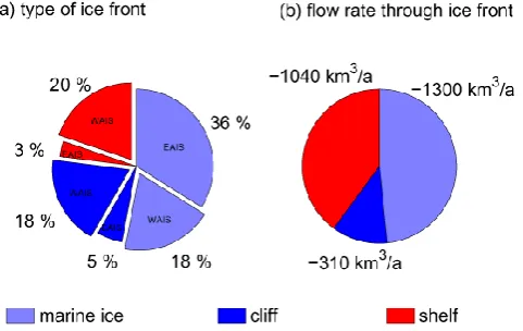
Fig. 9. (a) Partitioning of the different types of ice fronts in the equilibrium simulation, and (b) their contribution to the mass bud-get. Note that an ice flow of−1190 km3a−1can be attributed to East Antarctica.
before the stresses are evaluated again at a grounded mar-gin. Figure 9b shows that most of the mass loss occurs at marine ice fronts and shelves. Only a small part occurs at cliffs (about 12 %) relative to their extent (23 % of the ice front of Antarctica is comprised of cliffs). Conversely, al-though shelves account for only 23 % of the total modeled ice front of Antarctica, they provide 39 % of the mass loss. This can be explained by the different magnitude of velocities in sheet and shelves which will be further discussed in Sect. 3.3. Also, in regions with high outflux the model tends to pro-duce ice shelves. The formation of shelves influences the grounded ice upstream and thereby the mass balance both by buttressing effects in the case of an embayment and through the drawdown of grounded ice. As shown in Sect. 3.1 the total ice shelf area in our simulation is smaller than in obser-vation. A subgrid treatment of grounded margins analogous to that for the calving fronts, and higher resolution, might improve this.
3.3 Steady state dynamics
The ice geometry, grounding line position, ice front position, and ice front type each evolve to an equilibrium at the end of the simulation. In Fig. 10 the surface velocities for this steady state are detailed for the West Antarctic Ice Sheet. In Fig. 11 the flow pattern for the whole Antarctic ice sheet is shown, with the onset of streams as defined by equation 6 marked by black lines. As described in Sect. 2 streams are (diagnostically) distinguished from the surrounding ice by comparing the sliding velocityvb=vSSAto the vertically
averaged velocityv¯: ifvb>v¯−vbthen we consider the flow
stream-like. The overall pattern of drainage basins is easily recognizable: for WAIS there is drainage into the Amundsen Sea sector, an area subject to accelerated thinning in reality (Thomas et al., 2004; Pritchard et al., 2009). A feature that can be roughly identified with Thwaites Glacier plays a more
Fig. 10. Modeled surface velocity for the West Antarctic Ice Sheet. White lines show the grounding-line position, thin black lines indi-cate ice streams according to inequality Eq. (6).
Fig. 11. Modeled vertically-integrated horizontal ice flux. Ice streams are outlined in black, grounding line position in white.
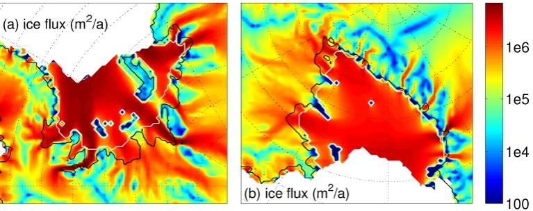
Fig. 12. Ice flux with streams indicated by black line for (a) Ronne-Filchner and (b) Ross Ice Shelves. The grounding line is marked by a white line.
Fig. 13. Comparison of surface velocity fields. (a) Observed surface velocities from MAMM data enriched by data from Joughin et al. (2002). (b) Surface velocities from equilibrium simulation. In both (a) and (b), regions without observational coverage and where there is no agreement in the simulation and the observations about whether the ice is grounded or floating are masked out, which leaves 65 % of total ice covered area for comparison. The respective grounding line positions and calving fronts for observation and model are depicted in black and red, as in Fig. 5.
shown in Fig. 8, indicating the strong influence of bottom to-pography on our simulation. Figure 12 shows the ice flux for the combined stream-shelf system for the two largest shelves. Due to the anomaly in the position of the grounding line the location of the stream-like features in the simulation cannot directly coincide with real streams in Antarctica. Combin-ing the SIA and SSA velocities as described in Sect. 2 is, however, shown to model stream-like features in a reason-able way.
In order to compare these model results to observational data we combined two sources, namely present-day surface velocities from both the Modified Antarctic Mapping Mis-sion (Jezek et al., 2003; Liu et al., 1999) and for the Siple Coast area of WAIS, from Joughin et al. (2002), see Fig. 13a. Regions where there is no agreement in the simulation and
M. A. Martin et al.: PISM-PIK – Part 2 737
Fig. 14. Point-by-point scatterplot of modeled and observed veloc-ities. The mean difference from modeled to observed velocities for grounded points is≈4 m a−1 with a standard deviation from this mean difference of≈81 m a−1. For floating points we get a larger difference of≈334 m a−1with a standard deviation of≈309 m a−1. The stars with red points are the floating velocities that belong to the Ronne-Filchner Ice-Shelf, while the ones with the cyan points be-long to the Ross Ice Shelf.
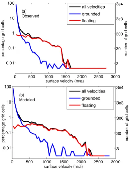
Fig. 15. Histogram of velocity distribution. (a) observed (b) modeled. Each of the 60 bins contains a velocity range of
1vsurface=50 m a−1.
Fig. 16. Histogram of velocity distribution. Panel (a) grounded and panel (b) floating areas (please note that the strongest overes-timation occurs only for a small number of grid cells). Relative to Fig. 15, we show results from the smaller dataset (Fig. 13), contain-ing only data where there is agreement between model and obser-vation about whether the ice is grounded or floating.
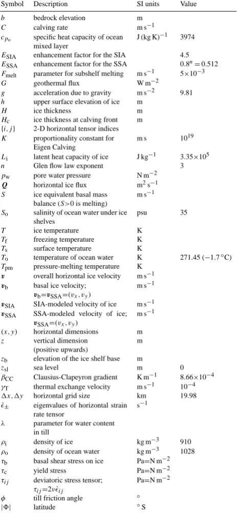
Table A1. Table of symbols and values of constants.
Symbol Description SI units Value
b bedrock elevation m
C calving rate m s−1
cpo specific heat capacity of ocean
mixed layer
J (kg K)−1 3974
ESIA enhancement factor for the SIA 4.5 ESSA enhancement factor for the SSA 0.8n=0.512
Fmelt parameter for subshelf melting m s−1 5×10⁻³
G geothermal flux W m−2
g acceleration due to gravity m s−2 9.81 h upper surface elevation of ice m
H ice thickness m
Hc ice thickness at calving front m {i,j} 2-D horizontal tensor indices
K proportionality constant for Eigen Calving
m s 1019
Li latent heat capacity of ice J kg−1 3.35×10⁵
n Glen flow law exponent 3
pw pore water pressure N m−2
Q horizontal ice flux m2s−1 S ice equivalent basal mass
balance (S>0 is melting)
m s−1
So salinity of ocean water under ice shelves
psu 35
T ice temperature K
Tf freezing temperature K
Ts surface temperature K
To temperature of ocean water K 271.45 (−1.7◦C) Tpm pressure-melting temperature K
v overall horizontal ice velocity m s−1
vb basal ice velocity;
vb=vSSA=(vx,vy)
m s−1
vSIA SIA-modeled velocity of ice m s−1
vSSA SSA-modeled velocity of ice;
vSSA=(vx,vy)
m s−1
(x,y) horizontal dimensions m
z vertical dimension (positive upwards)
m
zb elevation of the ice shelf base m
zsl sea level m 0
βCC Clausius-Clapeyron gradient K m−1 8.66×10⁻⁴ γT thermal exchange velocity m s−1 10−4 1x,1y horizontal grid size km 19.98 ˙
± eigenvalues of horizontal strain
rate tensor
s−1
λ parameter for water content in till
ρi density of ice kg m−3 910 ρo density of ocean water kg m−3 1028
τb basal shear stress on ice Pa=N m−2 τc yield stress Pa=N m−2 τij deviatoric stress tensor;
τij=2ν˙ij
Pa=N m−2
φ till friction angle ◦
|8| latitude ◦S
are too numerous in the simulation, but the strongest over-estimation occurs only in a small number of grid cells. For grounded grid cells the model gives more realistic values (see also Fig. 14).
4 Conclusions
Our dynamic equilibrium simulation for Antarctica demon-strates the ability of PISM-PIK to reproduce large-scale dy-namic features of the Antarctic ice sheet-shelf system, in-cluding observed features such as the fast flow of ice streams and the position of ice fronts. A comparison of the geometry and dynamics in modeled equilibrium using observed surface velocities covering≈65 % of the ice-covered area supports the PISM-PIK treatment of the calving front and its direct superposition of SIA and SSA. These new techniques cap-ture the full range of fast-flowing ice in the whole sheet/shelf system. This hybrid scheme leads to a smooth transition from sheet to shelves and permits a diagnostic definition of streams (Fig. 2). The mass budget of Antarctica in simu-lated steady state was analyzed, identifying the composition of mass loss at different types of ice fronts (Fig. 9). Though subgrid interpolation is used in PISM-PIK for the floating parts of the calving front (Albrecht et al., 2011), it is cur-rently not used for locations where the model has grounded ice margins. This may be the explanation for a reduced area of floating ice in the model relative to observations (Table 1). The formation of an attached shelf influences the grounded ice upstream, both by buttressing effects in the case of an embayment and the draw-down of grounded ice because of high shelf velocities being transmitted by membrane stresses into the upstream grounded ice. Additional subgrid treatment may improve grounded marine margins in future model ver-sions. Significant additional improvements, particularly with respect to grounding line position (Fig. 6), ice thickness dis-tribution (Fig. 7), and velocity disdis-tribution (Figs. 10–16), are expected from finer grid resolution, improved topographic input data, and additional information on the dynamic basal boundary conditions (basal shear stress) of grounded ice.
Supplementary material related to this article is available online at:
http://www.the-cryosphere.net/5/727/2011/ tc-5-727-2011-supplement.zip.
Acknowledgements. M. Haseloff and T. Albrecht were funded
by the German National Academic Foundation; M. A. Martin and R. Winkelmann by the TIPI project of the WGL. R. Winkel-mann acknowledges support by the IMPRS-ESM. E. Bueler and C. Khroulev are supported by NASA grant NNX09AJ38G. We thank Jed Brown (ETH Zurich, Switzerland) for advice on PISM, and the anonymous referees and editor Hilmar Gudmundsson for their helpful comments on the original manuscript.
M. A. Martin et al.: PISM-PIK – Part 2 739
References
Albrecht, T., Martin, M., Haseloff, M., Winkelmann, R., and Lever-mann, A.: Parameterization for subgrid-scale motion of ice-shelf calving fronts, The Cryosphere, 5, 35–44, doi:10.5194/tc-5-35-2011, 2011.
Arthern, R. J. and Gudmundsson, G. H.: Initialization of ice-sheet forecasts viewed as an inverse Robin problem, J. Glaciol., 56, 527–533, 2010.
Bamber, J. L., Vaughan, D. G., and Joughin, I.: Widespread Com-plex Flow in the Interior of the Antarctic Ice Sheet, Science, 287, 1248–1250, 2000.
Beckmann, A. and Goosse, H.: A parametrization of ice shelf-ocean interaction for climate models, Ocean Model., 5(2), 157–170, 2003.
Bueler, E. and Brown, J.: The shallow shelf approximation as a sliding law in a thermomechanically coupled ice sheet model, J. Geophys. Res., 114, F03008, doi:10.1029/2008JF001179, 2009. Bueler, E., Brown, J., and Lingle, C.: Exact solutions to the thermo-mechanically coupled shallow-ice approximation: effective tools for verification, J. Glaciol., 53, 499–516, 2007.
Bueler, E., Khroulev, C., Aschwanden, A., Joughin, I., and Smith, B. E.: Modeled and Observed Fast Flow in the Greenland Ice Sheet, 2010.
Clarke, G. K. C.: Subglacial Processes, Annu. Rev. Earth Pl. Sc., 33, 247–276, 2005.
Comiso, J. C.: Variability and Trends in Antarctic Surface Tem-peratures from In Situ and Satellite Infrared Measurements, J. Climate, 13, 1674–1696, 2000.
Goldberg, D. N. and Sergienko, O. V.: Data assimilation us-ing a hybrid ice flow model, The Cryosphere, 5, 315–327, doi:10.5194/tc-5-315-2011, 2011.
Hellmer, H. H. and Olbers, D. J.: A Two-Dimensional Model for the Thermohaline Circulation Under an Ice Shelf, Antarct. Sci., 1(04), 325–336, 1989.
Holland, D. M. and Jenkins, A.: Modeling Thermodynamic Ice-Ocean Interactions at the Base of an Ice Shelf, J. Climate, 29, 1787–1800, 1999.
Hulbe, C. L. and MacAyeal, D. R.: A new numerical model of cou-pled inland ice sheet, ice stream, and ice shelf flow and its ap-plication to the West Antarctic Ice Sheet, J. Geophys. Res., 104, 25349–25366, 1999.
Huybrechts, P.: A 3-D model for the Antarctic ice-sheet: a sensi-tivity study on the glacial-interglacial contrast, Clim. Dynam., 5, 79–92, 1990.
Huybrechts, P.: Glaciological modellint of the late Cenozoic East Antarctic Ice Sheet: Stability or dynamism, Geogr. Ann., 75A(4), 221–238, 1993.
Jezek, K. C., Farness, K., Carande, R., Wu, X., and Labelle-Hamer, N.: RADARSAT 1 synthetic aperture radar observations of Antarctica: Modified Antarctic Mapping Mission, 2000, Ra-dio Sci., 38, 32–1, 2003.
Joughin, I., Tulaczyk, S., Bindschadler, R., and Price, S. F.: Changes in west Antarctic ice stream velocities: Observation and analysis, J. Geophys. Res.-Sol. Ea., 107, 2289 pp., EPM 3-1–3-22, 2002.
Joughin, I., Tulaczyk, S., Bamber, J., Blankenship, D., Holt, J., Scambos, T., and Vaughan, D.: Basal Conditions for Pine Island and Thwaites Glaciers Determined using Satellite and Airborne Data, J. Glaciology, 55(190), 245–257, 2009.
Le Brocq, A. M., Payne, A. J., and Vieli, A.: An im-proved Antarctic dataset for high resolution numerical ice sheet models (ALBMAP v1), Earth Syst. Sci. Data, 2, 247–260, doi:10.5194/essd-2-247-2010, 2010.
Levermann, A., Albrecht, T., Winkelmann, R., Martin, M. A., and Haseloff, M.: Universal Dynamic Calving Law implies Potential for Abrupt Ice-Shelf Retreat, submitted, 2011.
Liu, H., Jezek, K. C., and Li, B.: Development of an Antarctic digital elevation model by integrating cartographic and remotely sensed data: A geographic information system based approach, J. Geophys. Res., 104, 23199–23214, 1999.
Lythe, M. B., Vaughan, D. G., and BEDMAP Consortium: BEDMAP: A new ice thickness and subglacial topographic model of Antarctica, J. Geophys. Res., 106, 11335–11351, 2001. Ma, Y., Gagliardini, O., Ritz, C., Gillet-Chaulet, F., Durand, G., and Montagnat, M.: Enhancement Factors for Grounded Ice and Ice-Shelves inferred from an anisotropic ice flow model, J. Glaciol., 56, 805–812, 2010.
Macayeal, D. R.: The basal stress distribution of ice stream E, Antarctica, inferred by control methods, J. Geophys. Res., 97, 595–603, 1992.
MacAyeal, D. R.: A tutorial on the use of control methods in ice-sheet modeling, J. Glaciol., 39(131), 91–98, 1993.
Maxwell, D., Truffer, M., Avdonin, S., and Stuefer, M.: An iter-ative scheme for determining glacier velocities and stresses, J. Glaciol., 54, 888–898, 2008.
Oerter, H., Kipfstuhl, J., Determann, J., Miller, H., Wagenbach, D., Minikin, A., and Graft, W.: Evidence for basal marine ice in the Filchner-Ronne ice shelf, Nature, 358(6385), 399–401, 1992. Paterson, W. S. B.: The Physics of Glaciers, Elsevier, Oxford, 1994. Pollard, D. and Deconto, R. M.: Modelling West Antarctic ice sheet growth and collapse through the past five million years, Nature, 458, 329–332, 2009.
Pritchard, H. D., Arthern, R. J., Vaughan, D. G., and Edwards, L. A.: Extensive dynamic thinning on the margins of the Green-land and Antarctic ice sheets, Nature, 461, 971–975, 2009. Raymond, M. J. and Gudmundsson, G. H.: Estimating basal
properties of ice streams from surface measurements: a non-linear Bayesian inverse approach applied to synthetic data, The Cryosphere, 3, 265–278, doi:10.5194/tc-3-265-2009, 2009. Ritz, C., Rommelaere, V., and Dumas, C.: Modeling the evolution
of Antarctic ice sheet over the last 420,000 years: Implications for altitude changes in the Vostok region, J. Geophys. Res., 106, 31943–31964, 2001.
Rott, H., M¨uller, F., Nagler, T., and Floricioiu, D.: The imbalance of glaciers after disintegration of Larsen-B ice shelf, Antarctic Peninsula, The Cryosphere, 5, 125–134, doi:10.5194/tc-5-125-2011, 2011.
Schoof, C.: Variational methods for glacier flow over plastic till, J. Fluid Mech., 555(-1), 299–320, 2006a.
Schoof, C.: A variational approach to ice stream flow, J. Fluid Mech., 556, 227–251, 2006b.
Schoof, C., Hindmarsh, R. C. A., and Pattyn, F.: MISMIP: Marine ice sheet model intercomparison project, http://homepages.ulb. ac.be/∼fpattyn/mismip/, 2009.
SeaRISE, Sea-level Response to Ice Sheet Evolution (SeaRISE), 2011.
application to Antarctica, Earth Planet Sc. Lett., 223, 213–224, 2004.
Thomas, R., Rignot, E., Casassa, G., Kanagaratnam, P., Acu˜na, C., Akins, T., Brecher, H., Frederick, E., Gogineni, P., Krabill, W., Manizade, S., Ramamoorthy, H., Rivera, A., Russell, R., Son-ntag, J., Swift, R., Yungel, J., and Zwally, J.: Accelerated Sea-Level Rise from West Antarctica, Science, 306, 255–258, 2004. Van de Berg, W. J., Van den Broeke, M. R., Reijmer, C. H.,
and Van Meijgaard, E.: Reassessment of the Antarctic sur-face mass balance using calibrated output of a regional atmo-spheric climate model, J. Geophys. Res.-Atmos., 111, D11104, doi:10.1029/2005JD006495, 2006.
Van den Broeke, M.: Depth and Density of the Antarctic Firn Layer, Arct. Antarct. Alp. Res., 40, 432–438, 2008.