A comparative study to estimate the parameters of mixed-Weibull distribution

A comparative study to estimate the

parameters of mixed-Weibull distribution

Arfa Maqsood

Department of Statistics, University of Karachi Karachi

Mohammad Aslam

Department of Statistics, University of Karachi Karachi

Abstract

A mixture of Weibull distribution, involving two shape parameters, two scale parameters, and one proportionality parameter, is simulated through the statistical software MINITAB (1996). The two methods Graphical (John H.K. Kao 1959) and moments based (Lee W. Fall 1970) are applied to estimate the underlying five parameters of mixed Weibull distribution in order to find the accuracy and precision of the estimator.

1. Introduction

The Weibull distribution, derived in 1939 by W. Weibull has been recognized as an appropriate model in reliability studies and life-testing problems such as time to failure or life length of a component or a product.

Distributions resulting from mixing two or more component distributions are designated as ‘mixed’ or ‘compound’. Some methods for obtaining efficient estimates of the mixed Weibull distribution have been outlined in recent years. A method for estimating parameters of mixed distributions using sample moments has been outlined by Paul R. Rider (1961) who considered compound Poisson, Binomial, and a special case of the mixed Weibull distribution. A graphical method for estimating the mixed Weibull parameters in life testing of electron tubes is proposed by John H. K. Kao (1959).

This paper presents a comparison of the estimation methods to find the accuracy and precision of the estimator. For this purpose we simulate the data from Weibull distribution using MINITAB (1996) and apply the two methods of estimating the parameters of mixed Weibull distribution.

1.1 Simple Weibull distribution

A simple Weibull probability distribution function is defined as

0 ; exp

) (

1

> ⎥ ⎥ ⎦ ⎤ ⎢

⎢ ⎣ ⎡

⎟ ⎠ ⎞ ⎜ ⎝ ⎛ ⎟

⎠ ⎞ ⎜ ⎝ ⎛ =

−

x x

x x

f

β β

α α

α β

The strength of the Weibull lies in its flexible shape as a model for many different kinds of data. The parameter β plays the role in determining, how the Weibull will look.

Table1: Weibull Distribution Properties

Shape Parameter PDF 0 < β < 1

β =1

β >1

β =2 3 ≤β≤ 4

β >10

Exponentially decay from infinity Exponentially decay from 1/mean Rises to peak and then decrease Reyleigh distribution

Has normal bell shape appearance

Has shape very similar to type 1 extreme value distribution

0 0.5 1 1.5 2 2.5 3

0 0.2 0.4 0.6 0.8 1 1.2 1.4 1.6 1.8

x

f(

x)

Weibull PDF Plot

beta=0.5 beta=1.0 beta=1.5 beta=3.0

Figure1: Shows some of the simple Weibull distribution for β = 0.5, 1, 1.5 and 3.

1.2 Mixed-Weibull Distribution

A k two-parametric Weibull probability distribution function is defined as

∑

∑

= =

= = k

i

k

i i i

if x P

P x

f

1 1

1 ;

) ( )

( Where;

) (

) (

parameter mixture

population sub

of proportion P

population sub

ith x f

i i

− ⇒

A mixture distribution involving two-two parametric Weibull distribution is

1 ;

) ( )

( )

(x =P₁f₁ x +P₂f₂ x P₁ +P₂ =

f

) ( ) 1 ( ) ( )

(x Pf₁ x P f₂ x

f = + − (1)

( ) exp (1 ) exp ; 0

2 2

1 1

2 1

2 2 2

1 1

1 1

1 >

⎪⎭ ⎪ ⎬ ⎫ ⎪⎩

⎪ ⎨ ⎧

⎟⎟ ⎠ ⎞ ⎜⎜ ⎝ ⎛ − ⎟⎟

⎠ ⎞ ⎜⎜ ⎝ ⎛ − + ⎪⎭ ⎪ ⎬ ⎫ ⎪⎩

⎪ ⎨ ⎧

⎟⎟ ⎠ ⎞ ⎜⎜ ⎝ ⎛ − ⎟⎟

⎠ ⎞ ⎜⎜ ⎝ ⎛ =

− −

x x

x P

x x

P x f

β β

β β

α α

α β α

α α

β ₍₂₎

Where;

α >0, scale parameter, β>0, shape parameter, P >0, mixture parameter

CDF of mixed- Weibull distribution is defined as

(3)

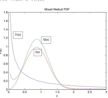
0 0.5 1 1.5 2 2.5 3

0 0.2 0.4 0.6 0.8 1 1.2 1.4 1.6 1.8

x

F(

x)

Mixed Weibull PDF

f1(x)

f2(x)

f(x)

Figure 2: Mixed Weibull probability density function (α1 = α2 = 1, p = 0.2, β1 = 0.5 and β2 = 3)

2. Estimation of the parameters of mixed-Weibull distribution

Numerous methods for obtaining efficient estimates of the simple Weibull distribution have been outlined in recent years; however we can not apply all these methods to the mixed-Weibull distribution due to complexity of the functional form. We therefore consider the two methods of estimation Graphical and Sample moments to find the accuracy and precision of the estimator.

) ( ) 1 ( ) ( )

(x PF₁ x P F₂ x

2.1 Graphical Method

A graphical procedure for estimation of mixed-Weibull parameters in life-testing of electron tubes is given by John H. K. Kao (1959). This method of estimating the parameters is based upon the fact that a Weibull cumulative distribution becomes a straight line in ln versus ln-ln coordinates.

1. Plot the sample cdf on Weibull probability paper and fit by inspection a smooth curve (called Weibull plot).

2. Starting from each end of the Weibull plot draw a tangent line and denote them by _pFˆ_{1 and}

2 ˆ ) 1

( − p F which are the estimates of pF1(x) and qF2(x) respectively.

3. At the intersection of (1−p)Fˆ2 with the upper boarder line drop a vertical line whose intersection with _pFˆ_{1as read from the percent failure scale} gives pˆ the estimate of p and hence 1-p=q.

4. Mixed Weibull distribution may now be separated into the two sub-populations. The estimated number of items belong to F1(x) and F2(x) are npˆ and nqˆ respectively from which the sample cdf’s of F1(x) and F2(x) may be calculated.

5. The y-intercept and slope of the plots of the separated sub-populations Fi(x), give the usual estimates of −βlnα_i and β_i respectively.

2.2 Method of sample moments

The rth theoretical moment about origin of the mixed Weibull distribution f(x) is

(4)

where fi(x) are defined as in equation (2).

The first five theoretical moments about origin follow as

1,2,3,4,5 r

for 1

) 1 ( 1

2 2 1

1 ⎟⎟ =

⎠ ⎞ ⎜⎜

⎝ ⎛

+ Γ −

+ ⎟⎟ ⎠ ⎞ ⎜⎜

⎝ ⎛

+ Γ = ′

β α β

α

μ p r r p r r

r (5)

Now equating the theoretical moments to the corresponding sample moments, the set of equations (5) becomes

1,2,3,4,5 r

for 1

) 1 ( 1

2 2 1

1 ⎟⎟ =

⎠ ⎞ ⎜⎜

⎝ ⎛

+ Γ −

+ ⎟⎟ ⎠ ⎞ ⎜⎜

⎝ ⎛

+ Γ =

β α β

α r p r

p

m_r r r (6)

Where mr is the sample moment about the origin.

∫

∫

∞

− + =

′

0 2 0

1(x)dx (1 p) x f (x)dx f

x

p r r

r

The set of equations (6) is a system of five equations which must be solved simultaneously for estimates of the five parameters p, α1, α2, β1, β2. For convenience in handling these equations, we will make the following transformations where necessary in this paper.

Let ⎟⎟ ⎠ ⎞ ⎜⎜ ⎝ ⎛ + Γ = ⎟⎟ ⎠ ⎞ ⎜⎜ ⎝ ⎛ + Γ

= 1 1 v 1 1

2 1

1

1 β β

u ⎟⎟ ⎠ ⎞ ⎜⎜ ⎝ ⎛ + Γ = ⎟⎟ ⎠ ⎞ ⎜⎜ ⎝ ⎛ + Γ

= 2 1 v 2 1

2 2

1

2 β β

u ⎟⎟ ⎠ ⎞ ⎜⎜ ⎝ ⎛ + Γ = ⎟⎟ ⎠ ⎞ ⎜⎜ ⎝ ⎛ + Γ

= 3 1 v 3 1

2 3

1

3 β β

u ⎟⎟ ⎠ ⎞ ⎜⎜ ⎝ ⎛ + Γ = ⎟⎟ ⎠ ⎞ ⎜⎜ ⎝ ⎛ + Γ

= 4 1 v 4 1

2 4

1

4 β β

u

Thus, the system of equations (6) becomes

r r r

r

r p u p v

m = α1 +(1− )α2 r =1, 2, 3, 4, 5 (7)

Solving equations (7) for r=1, 2 to obtain the estimates ofα1andα2, yields

2 1 2 2 1 2 2 2 4 1 2 2 2 1 2 2 1 2 2 2 2 1 2 2 1 1 2 1 2 ) 1 ( ) 1 ( ) 1 ( ) 1 ( ) 1 ( ) 1 ( ˆ u v p p v u p v u m p p v u u m p p u u v m p p v u p m − + − − + − + − − ± − =

α (8)

⎥ ⎥ ⎦ ⎤ ⎢ ⎢ ⎣ ⎡ − + − − + − + − − ± − − − = ₂ 1 2 2 1 2 2 2 4 1 2 2 2 1 2 2 1 2 2 2 2 1 2 2 1 1 2 1 1 1 1 1 1 ) 1 ( ) 1 ( ) 1 ( ) 1 ( ) 1 ( ) 1 ( ) 1 ( ˆ u v p p v u p v u m p p v u u m p p u u v m p p v u p m pu v p pu m

α (9)

Substituting the expression of α1andα2in the next two equations, obtained from the system of equations (7) for r = 3 and 4, there are now two equations and three unknowns. At this point, the explicit expressions for the unknown parameters p, β1, β2 can not be obtained. Therefore the graphical method is used to obtain the estimate of p, the proportionality parameter. Once an estimate of p has been determined graphically, solve the two equations for β1,and β2 by the Newton–Raphson method for solving non-linear system of equations (NRSYS), defined as follows

) ( ) ( dx where _k 1

1 k k k k

k x dx f x f x

x ₊ = + = − ′ −

Where;

⎥ ⎥ ⎥ ⎥

⎦ ⎤

⎢ ⎢ ⎢ ⎢

⎣ ⎡

∂ ∂ ∂

∂

∂ ∂ ∂

∂

= ′ ⎥

⎦ ⎤ ⎢

⎣ ⎡ = ⎥

⎦ ⎤ ⎢ ⎣ ⎡ =

) , (

) , (

) , (

) , ( )

( )

, (

) , ( ) (

2 1 2 2 2

1 2 1

2 1 1 2 2

1 1 1

2 1 2

2 1 1

2 1

β β β β

β β

β β β β

β β β

β β

β β β

β β β

f f

f f

f f

f f

Hence,

) ( )

( 1

1 k k k

k β f β f β

β −

+ = − ′ (10)

Once β1,and β2have been determined by the equation (10), estimates of

2 1 andα

α are obtained from equation (8) and (9) respectively.

3. Simulation from MINITAB

We simulate a random sample of size 100 in such a way that in the sample first 40 values have parametric values β1=0.5 and α1=1, and last 60 values have parametric values β2=2.5 and α2=10. The proportion of first 40 values is 40/100 = 0.4 and hence 1-p = q = 0.6.

3.1 Estimation by Graphical Method

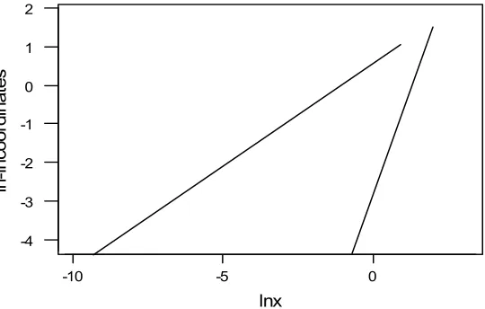
Figure 4 shows the Weibull cumulative plots of the separated sub-population Fi(x). The y-intercepts and slopes of the two straight lines are determined and hence the estimates of the remaining parameters are

2 1

2

1 α β β

α

0.85 10.7 0.47 2.35

3.2 Estimation by Method of moments

The iterations from the set of equations (8), (9), and (10) are obtained, as follow

Table 2: Iteration values

β1 β2 α1 α2

0.5 1 1.393712 8.362272

0.38687 1.47451 0.315633 10.39815 0.38068 2.14614 0.243961 10.77967 0.41655 3.17987 0.367359 10.54711 0.48625 1.89023 0.865206 10.11597 0.52899 2.56534 1.090066 10.0033

0 -5

-10 2

1

0

-1

-2

-3

-4

lnx

ln

-ln

coo

rd

inat

es

Figure 4: ln versus ln-ln coordinates

4. Conclusion

Table 3: Summarizes the results obtained by all concerned methods

Parameters

Graphical Moments

Estimates Sampling _error Estimates Sampling _error

P 0.4 0.39 0.01 0.39

(graphical) 0.01

1

α 1 0.85 0.15 1.09 0.09

2

α 10 10.7 0.7 10.0 0

1

β 0.5 0.47 0.03 0.52 0.02

2

β 2.5 2.35 0.15 2.56 0.06

5. References

1. Bain Lee J., and Engelhardt M. (1992). “Introduction to Probability and Mathematical Statistics”, Ed. 2nd, Duxbury Press, California.

2. Cohen, A. C., JR. (1965).”Estimation in Mixtures of Two Normal Distributions”, University of Georgia, Institute of Statistics, TR No. 13.

3. Falls Lee W. (1970). “Estimation of Parameters in Compound Weibull Distributions”, Technometrics pp 399-407, Vol. 12, No. 2.

4. Hogg. Robert V, and Craig Allen T. (1995). “Introduction to Mathematical Statistics”, Ed. 5th_{, John Wiley.}

5. Kao, J. H. K. (1959). “A Graphical Estimation of Mixed Weibull Parameters in Life- Testing of Electron Tubes”, Technometrics 1, pp 389-407.

6. Menon, M. V. (1963). “Estimation of the Shape and Scale Parameters of the Weibull Distribution”, Technometrics 5, pp 175-182.

7. Minitab, (1996), Statistical Software Release 12 Minitab. Inc. State College, P.A. 16801 USA.

8. Murthy, D.N.P. and Jiang R. (1998). “Mixture of Weibull Distribution Parametric Characterization of Failure date Function”, pp 47-65, John Wiley and Sons. Ltd.

9. Rider, Paul R. (1961). “Estimating the Parameters of Mixed Poisson, Binomial and Weibull Distributions by the method of moments”, Bulletin de l'institute international de statistique 38, part 2.