Structural and Magnetic Phases in Pressure-Tuned Quantum Materials

Structural and Magnetic Phases in

Pressure-Tuned Quantum Materials

David Matthew Jarvis

Dr S. S. Saxena

Department of Physics

University of Cambridge

This thesis is submitted for the degree of

Doctor of Philosophy

Declaration

This thesis is the result of my own work and includes nothing which is the outcome of work done in collaboration except as declared in the Preface and specified in the text. It is not substantially the same as any that I have submitted, or, is being concurrently submitted for a degree or diploma or other qualification at the University of Cambridge or any other University or similar institution except as declared in the Preface and specified in the text. I further state that no substantial part of my thesis has already been submitted, or, is being concurrently submitted for any such degree, diploma or other qualification at the University of Cambridge or any other University or similar institution except as declared in the Preface and specified in the text. It does not exceed the prescribed word limit for the relevant Degree Committee.

David Matthew Jarvis September 2020

Abstract

Structural and Magnetic Phases in Pressure-Tuned Quantum Materials

David Matthew Jarvis

This thesis presents work exploring the use of pressure as a tuning parameter for exploring the phase diagrams and properties of magnetically ordered insulators, to add understanding to several areas of current interest in condensed matter research. It shows the versatility of pres-sure as an experimental technique for exploring material properties free from complicating factors which arise with similar techniques such as chemical doping.

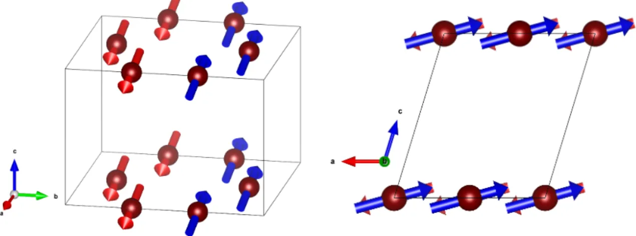
The properties of low-dimensional magnetic materials, and how these systems respond as they are pushed toward a more three-dimensional nature is explored through studies of both the crystal and magnetic structures of the family of quasi-two-dimensional magnetic insulatorsMPS3(M=Fe, Ni, Mn). With previous work largely being specific to individual

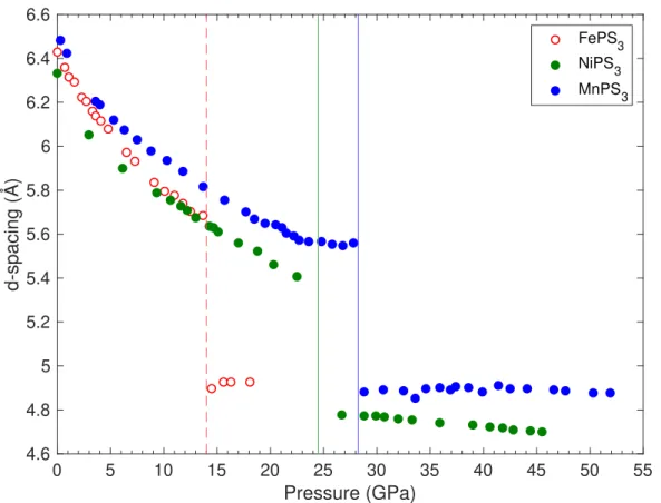
compounds, this thesis contributes to a more unified understanding of their properties. It shows that Ni and MnPS3 undergo similar structural transitions under pressure to those

previous observed in FePS3, the highest pressure of which is linked to an insulator-to-metal

transition in that system. Through record high-pressure neutron diffraction measurements, the evolution of the antiferromagnetic order in FePS3through this metallisation is studied for

the first time. In contradiction to previous indirect measurements, it is seen that magnetism persists into the metallic phase, with long range antiferromagnetism giving way to a previ-ously unobserved short-range order. This work is relevant on a broader scale for numerous layered magnetic materials such as cuprate high temperature superconductors.

Secondly, pressure is used to explore the magnetocaloric properties of the antiferromagnet EuTiO3. Recent work has shown that this compound compares favourably to many materials

commonly used in magnetic refrigeration. Measurements show that these properties are suppressed by the application of pressure and point towards the potential existence of a previously undiscussed transition in the material between 0.4 GPa and 0.5 GPa.

Acknowledgements

There are many people to whom I owe sincere thanks for helping to make this work possible. I am extremely grateful to my supervisor Montu Saxena for his continual support, guidance and the many opportunities which I have had thanks to him. I would have very few results to discuss were it not for the constant support and endless patience of Cheng Liu, whose guidance has helped bring so much of this work to fruition. To Matt Coak and Phil Brown I am very grateful for not only their scientific contributions and exceedingly helpful software for analysis, but also for pulling me through and always being there with a positive word.

Members of QM, Siân Dutton, Patricia Alireza, Keiron Murphy, Jiasheng Chen and many others have always been incredibly generous in offering both advice and assistance and I have benefited no end from their range of expertise. With the facilities experiments in both planning and execution I am indebted to Andrew Wildes and Thomas Hansen at the ILL, Dominik Daisenberger at Diamond and Helen Walker at ISIS.

Thanks go to the friends I have made here at Jesus College and in Cambridge who have made my time spent here so enjoyable: Phil and Ruth, Harry and Olga, Ramsay and James, Taylor, Bee, Darren and many others. Thanks to Keenan (and Rory and Kiera) for keeping me sane in the latter stages of writing.

For helping me get here and for always supporting me in my research and the writing of this thesis I cannot express my gratitude enough to my wife Robyn who has listened to me tirelessly whether I have been excited or complaining. Finally, thank you to my parents, Andrew Jarvis and Amanda Williams, for always being behind me, encouraging my interest in science and helping me through everything to get to this point.

Table of contents

1 Introduction 1

1.1 Quantum Criticality . . . 1

1.2 Low-dimensional Magnetic Materials . . . 3

1.3 Magnetocalorics . . . 7 2 Theoretical background 11 2.1 Low-dimensional Magnetism . . . 11 2.1.1 Metal-Insulator Transitions . . . 12 2.2 Magnetic Superexchange . . . 14 2.3 Quantum Criticality . . . 15

2.4 The Magnetocaloric Effect . . . 18

3 Methods 23 3.1 SQUID Magnetometry . . . 23

3.2 Synchrotron X-ray Experiments . . . 26

3.2.1 Powder X-ray Diffraction (PXRD) . . . 26

3.2.2 Single Crystal X-ray Diffraction . . . 28

3.3 Neutron Scattering . . . 29

3.3.1 Powder Neutron Diffraction . . . 29

3.4 High Pressure Methods . . . 31

3.4.1 SQUID Piston Cylinder Cell . . . 31

3.4.2 Diamond Anvil Cell . . . 34

4 MPS3Compounds 37 4.1 Overview of Previous Work . . . 37

4.1.1 Aims . . . 49

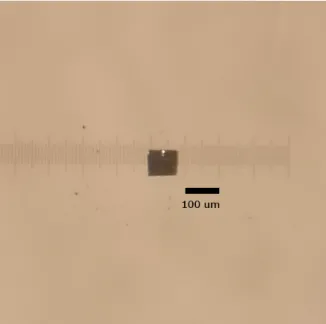
4.2 Preparation of samples . . . 50

x Table of contents

4.3.1 High Pressure Crystal Structures . . . 51

4.3.2 Single Crystal results . . . 59

4.3.3 High Pressure Magnetic Structure of FePS3 . . . 63

4.4 Discussion . . . 78

5 Magnetocaloric Properties of EuTiO3 85 5.1 Overview of Previous Work . . . 85

5.1.1 Aims . . . 89 5.2 Preparation of Samples . . . 89 5.3 Results . . . 91 5.4 Discussion . . . 101 6 Conclusions 103 6.1 MPS3Outlook . . . 103 6.2 ETO Outlook . . . 106

7 Search for superconductivity in theMPS3andMPSe3systems 109

Chapter 1

Introduction

This thesis explores the effective use of pressure as a tuning parameter for exploring the phase diagrams of magnetically ordered materials. The effect of pressure is to tune the underlying crystal structure of the materials. This direct manipulation of the crystal lattice may induce a great number of changes in both magnetism and the electrical properties of materials, modifying for instance magnetic exchange parameters by changing the relative positions and separation of ions.

A key advantage of pressure as a tuning parameter for exploring physical properties lies in its cleanliness. Other comparable methods such as chemical doping or substitution may directly change the occupation of electronic bands in the material and thereby influence their electrical and magnetic characteristics. With the use of hydrostatic pressure, only the crystal structure itself is directly modified, and therefore any changes in other material properties arise from this changing of the atomic unit cell in real space. In this way, the energies of bands in the electronic structure are modified, giving rise to various measurable effects.

Such manipulation of physical systems allows for a great number of questions in con-densed matter physics to be explored. A variety of model systems may be used to explore the behaviour of materials as high temperature superconductors, multiferroics and compounds exhibiting low-dimensional magnetic order.

1.1

Quantum Criticality

In using pressure as a tuning parameter in magnetic materials, the critical temperature for transitions between ordered and disordered states may be modified. The appearance of a quantum critical point follows from the continued suppression of a second order phase transition towards absolute zero temperature and brings to the fore several of the key aspects of the study of phase transitions in condensed matter physics. In a second order transition at

2 Introduction

finite temperature, thermal fluctuations in the system are responsible for destabilising order in the system by overcoming the reduction in entropy for which the order is responsible, or the free energy in the system. A second order phase transition may be driven to lower temperature by some tuning parameter such that the transition occurs at zero temperature, arriving at a quantum critical point (QCP) in the phase diagram. At low temperatures near to this point, thermal fluctuations are negligible in energy and it is instead quantum fluctuations between the ordered and disordered state which act to destabilise order. In addition, as the QCP exists at zero temperature, the third law of thermodynamics requires that the ordered and disordered phase be of equal entropy. This implies the existence of some form of order in the "disordered" phase.

The fluctuations in a system’s order parameter due to these quantum effects can result a number of emergent effects dependent on the nature of the material, which can persist up to unintuitively high temperatures despite the absolute zero temperature nature of their origin. Such effects include the emergence of unconventional superconductivity and other new forms of electric or magnetically mediated order.

Pressure has long been used as a tuning parameter to explore quantum critical phenomena in magnetically ordered systems. The suppression of either ferromagnetic or antiferromag-netic transition temperatures towards a quantum critical point at absolute zero temperature reveals the emergence of new behaviours including the emergence of unconventional super-conductivity in, for example, the ferromagnetic pure system UGe2[1]. A pressure-temperature

phase diagram of this material is shown in figure1.1.

This emergent superconductivity in UGe2is seen to coexist with the bulk ferromagnetism

in the material, and whilst the trend of the magnetic transition temperature with pressure is continuous, the transition to a ferromagnetic state is seen to become first-order below the expected pressure of the QCP. This change prevents experimental access to the precise pressure of the QCP, due to it being an effect unique to second-order transitions.

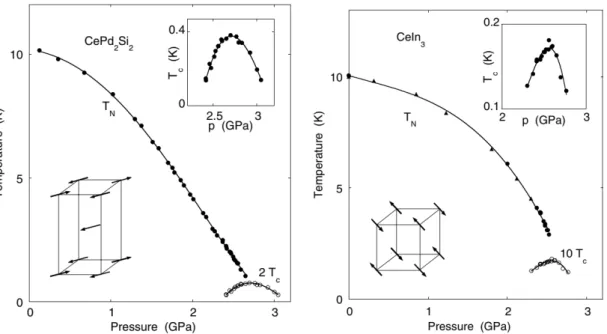
Similar behaviour is observed in antiferromagnetic materials such as CePd2Si2and CeIn3

in which superconductivity similarly emerges around an antiferromagnetic QCP[2]. Besides superconductivity, other new electronic behaviour is revealed at high pressures such as changes in the behaviour of resistivity with temperature away from the metallicT2exponent expected from traditional Fermi liquid theory.

Quantum critical effects are not however limited to magnetic materials, with recent work using pressure to demonstrate a number of effects in ferroelectric materials[3, 4,

5]. Such work provides further examples of the coupling of quantum critical effects with other excitations in a system. Quantum effects are significant event at ambient pressures in the quantum paraelectric class of materials, existing under ambient conditions near to a

1.2 Low-dimensional Magnetic Materials 3

Fig. 1.1 Pressure-Temperature phase diagram of the heavy-fermion superconductor UGe2.

The emergence of superconductivity under pressure in this compound follows the suppression of the Curie temperature towards zero at a ferromagnetic quantum critical point. Taken from reference [1].

quantum critical point in their phase diagram. With electrons in these ferroelectrics being non-itinerant, the ferroelectric quantum critical point may be approached without the emergence of superconductivity or the transitions becoming measurably first order.

1.2

Low-dimensional Magnetic Materials

A particular class of magnetically ordered systems which have yielded a great deal of new physics under pressure is that of low-dimensional magnetic insulators. High-temperature cuprate superconductors are key examples of this in which an insulating antiferromagnetic phase is gradually suppressed, with unconventional superconductivity emerging as the ground state system appears to approach a quantum critical point.

The antiferromagnetic heavy-fermion compounds discussed previously are also relevant in this context. Side-by-side, CePd2Si2and CeIn3illustrate the prediction from mean-field

theory that magnetically mediated superconductive pairing becomes more robust on moving from a cubic to a more tetragonal symmetry[6, 7, 8, 9]. Both the maximum T_c and the pressure range over which superconductivity is observed is larger in the tetragonal CePd2Si2

than in CeIn which has a cubic symmetry. This evolution of pairing as ones moves away from a cubic system is taken to the extreme in materials like the highT_c superconductors

4 Introduction

Fig. 1.2 Temperature-pressure phase diagrams for two antiferromagnetic systems which show superconductivity under pressure. Taken from reference [2].

which may be considered as quasi-two-dimensional systems with very limited interactions along one direction.

The phase diagrams of such cuprate highT_csuperconductors are often very complex: with the suppression of antiferromagnetic order comes not only unconventional superconductivity but new behaviour at higher temperatures in the so called pseudogap regime which remains poorly understood, such as an unusual density of states at the Fermi energy. Whilst much work on the cuprate family of high-temperature superconductors has focussed on the use of chemical doping as a tuning parameter, pressure has previously been used in tandem to explore the phase diagram of these complex materials[10]. Pressure can be used to access regions of the phase diagram which are difficult to reach using chemical techniques, including the high doping terminus of the superconducting dome in YBCO which is above the maximum hole concentration which can be achieved with oxygen doping.

The phase diagrams of the aforementioned heavy-fermions are broadly simpler than those of the cuprate superconductors. As such, these systems can act as models for the effects of pressure and doping in more complex materials, with the important distinction that the heavy-fermion compounds are not insulating in the antiferromagnetic phase, which prevents some direct comparison.

The family of materialsMPS3, where M is a first-row transition metal ion, provides a

wide space for exploring how quasi-two-dimensional magnetic insulators respond in terms of magnetic, electric and structural properties as pressure is used to push them towards a more

1.2 Low-dimensional Magnetic Materials 5

three dimensional nature. In this instance this change is achieved as the separation of the weakly coupled van der Waals planes is more easily reduced than distances within the planes, resulting in inter-planar interactions no longer being effectively negligible. With a range of model magnetic behaviour from Heisenberg to Ising to more complex interactions achievable in this family by varying the transition metal species, the evolution of each of these systems under pressure may be studied. The use of pressure here again highlights the importance of the crystal structure for the properties of this family. New physics in both electric and magnetic order may be accessed solely through manipulation of the structure and phonons, without artificial changes of valence, bonding or other properties through such techniques as chemical doping.

Alongside their varied magnetic structures this family of materials exhibit interesting electrical behaviour, being either Mott or charge-transfer insulators which simple band calculations predict to be metallic but in experiment being extremely insulating under ambient conditions. Some of these insulating phases are seen to give way to metallic behaviour under pressure as good examples of Mott insulator-metal transitions. A great deal of work remains to be done however to explore how these transitions are related to observed structural transitions under pressure and how these differ between members of the family. The combination of behaviours in both magnetism and conduction allows for a great variety of physics to be tested in systems which are free from impurities and other more complex behaviours. A temperature-pressure phase diagram of FePS3is shown in figure1.3, which

shows the rich range of electrical and magnetic behaviour which accompanies structural transitions in the compound.

Consideration of the model of magnetically mediated superconductivity further motivates interest in the MPS3 family of materials, being model two-dimensional antiferromagnets,

which under pressure have been seen to become metallic. The observation of supercon-ductivity under pressure alongside a structural transition in the related FePSe3supports the

notion that these materials are an ideal space in which to explore magnetically mediated superconductivity alongside the crossover from two to three-dimensional magnetism. Many materials of interest which show high temperature superconductivity are extremely complex and are commonly affected by the presence of impurities and imperfections in the crystal lattice. This, combined with how the emergence of effects such as superconductivity can mask physics occurring in the underlying state, motivates study of simpler systems such as theMPS3family which share common behaviour of interest. More than this, the study of the

phase diagrams of low-dimensional magnetic materials has revealed other new behaviours besides unconventional superconductivity. The action of pressure in these two-dimensional crystals to effectively push them towards a more three-dimensional character by modifying

6 Introduction

Fig. 1.3 Phase diagram of the quasi-two-dimensional antiferromagnet FePS3. Changes in

magnetic order accompany structural transitions under pressure as the system is pushed towards a more three dimensional nature. Metallisation coincides with the loss of long range magnetic order.

1.3 Magnetocalorics 7

inter-layer spacing, is seen to be strongly linked to the observed Mott insulator-to-metal transitions and the emergence of superconductivity but the precise mechanisms of this link remain to be explored. Many parallels may be drawn then between simpler model systems of this type, and the more complex highTccompounds as well as a number of other systems,

beyond simply electric or magnetic order to a more complete understanding of the structures as a whole. Studying these compounds under extremes of pressure and temperature is an effective step between some of the previously examined simple model systems and materials such as the high temperature superconductors, and understanding here will help to shed light on this area of extensive current interest.

1.3

Magnetocalorics

The magnetocaloric effect has for many years been exploited in research as a companion and extension to other methods of cryogenic refrigeration. The adiabatic demagnetisation refrigerator (ADR), utilising the magnetocaloric effect in a cycle has a number of advantages over the use of liquid cryogens such as 4He, 3He and dilution refrigerators exploiting a mixture of these.

Foremost for ease of use, ADRs do not necessarily require a continuous supply of helium, and so when paired with other dry cryogenic technologies such as pulse-tube refrigerators, allow for cooling from room temperature to millikelvin temperatures with a closed loop system alone, removing requirements of cryogen transport and the recapturing of boil off vapour. In contrast, the cost for the use of these systems is predominantly the cost of electricity for powering helium compressors and magnet power supplies.

The base temperature of an ADR, effective starting temperature and other characteristics depend on the magnetocaloric properties of the material used in the system, and as such the choice of this pill material is vital for optimising the capabilities of an ADR system. With the use of these systems expanding not just in research but into more commercial purposes, it is desirable that systems can be designed for specific capabilities and lifespan. More than ever this motivates the study of materials for this use to allow for the magnetocaloric effect to be exploited. Alongside the development of new materials with this purpose in mind, the study of how existing materials may be tuned or modified to enhance their magnetocaloric properties is also of use, and through changing the magnetic exchange parameters by manipulation of the lattice, pressure is a valuable tool for exploring magnetocaloric materials in this way.

EuTiO3(ETO) has attracted interest in recent year for its favourable properties for use in

magnetic refrigeration about the temperature required for the liquefaction of hydrogen. It has also been demonstrated that the magnetism in ETO is strongly linked to both its crystal

8 Introduction

structure and the incipient ferroelectricity also present in the system, and each of these may be controlled by the application of a field which couples to the other systems.

Such perovskite oxides showing quantum paraelectricity have recently demonstrated new behaviour under pressure linked to the theoretical ferroelectric quantum critical point. The dependence of the dielectric behaviour on temperature is changed by coupling between the soft phonon which would give rise to ferroelectricity and and other phonon modes in the system. The addition of magnetism to this interaction is a valuable next step to build a proper theoretical framework, and this investigation will be valuable to examine such a material as ETO is suitable for the continued development of this theory. The near-multiferroic nature of ETO is also of interest in light of predictions of unusual coupling between the dielectric and magnetic when both systems are tuned towards their respective quantum critical points. Whilst achieving this may require the application of two or more tuning parameters such as an external electric field alongside pressure, studying how the magnetism in this compound is affected by tuning its crystal structure by hydrostatic pressure is valuable as a stepping stone to a full study of potential multiferroic quantum criticality in the system. Simultaneously, the lens of magnetocaloric properties is a valuable way to explore related magnetic properties in this compound.

This is again linked back to the magnetocaloric effect in ETO by work demonstrating an increase in magnetic entropy useful for cooling in materials driven towards magnetic quantum critical points[11,12]. This concept has been demonstrated in magnetocaloric materials in both model low-dimensional systems and more typical three-dimensional magnets which are driven to a critical point by the application of magnetic field. The potential exploration of this effect in materials with an added layer of complexity in the form of potential charge ordering is further reason to to examine the magnetocaloric effect in materials such as ETO which are quantum paraelectrics and may potentially be pushed towards magnetic quantum criticality by turning parameters other than magnetic field.

Together the materials presented in this work present a valuable opportunity for exploring the coupling of magnetism and crystal structure in a range of both effective dimensionality and coupling between magnetic and electrical ordering. Furthermore, studying how magnetism evolves across metal-to-insulator transitions probes new physics which will be valuable for the study of emergent superconductivity in related compounds. To achieve this goal, a number of related developments in measuring both magnetic susceptibility and structure under extreme conditions will also be explored and implemented.

By examining both materials with low-dimensional magnetic order and those with significant magnetocaloric properties, the work presented here will explore how the direct

1.3 Magnetocalorics 9

manipulation of the crystal lattice allows for exploration of new phases, and the discussion of new emergent behaviours in insulating magnetic systems.

Chapter 2

Theoretical background

2.1

Low-dimensional Magnetism

For the case of localised wavefunctions where the hopping integral is small, a Heisenberg Hamiltonian may be used to describe the magnetic systems. Thus it is most applicable for insulators, and metals are not well described with it.

The magnetic exchange parameter in this model may be written as

J≃2JD−4

t2

U (2.1)

whereJ_Dis the exchange integral responsible for ferromagnetism in the systems andt is the small hopping integral which leads to antiferromagnetism.

A Heisenberg Hamiltonian for two spins may be defined as

H_H=−JS₁·S₂ (2.2)

which can equally be rewritten as

H_H =−J S_1xS_2x+S_1yS_2y+S_1zS_2z. (2.3) This can be further generalised by allowing for variation of the relative strengths of thex, yandzcomponents as H=−Jα S1xS2x+S1yS2y +βS1zS2z . (2.4)

The nature of the Hamiltonian then depends on the values of the constantsα andβ. α = β =1 recovers the isotropic Heisenberg Hamiltonian;α ̸=β ̸=0 an anisotropic Heisenberg; α =1,β =0 the XY Hamiltonian andα =0,β =1 the Ising Hamiltonian.

12 Theoretical background

2.1.1

Metal-Insulator Transitions

Separation between insulating and conductive behaviour may be initially seen in the ap-proximation of nearly free electrons in crystalline materials[13]. In this model insulators are materials where all energy bands are completely empty or filled, due to the fact that for every state with wave function ψ =eikxu(x,y,z) there is also an occupied state with ψ =e−ikxu∗(x,y,z). Contrarily, materials in which one or more energy bands are partially

filled are metals. This filling arises from the exclusion principle as only two electrons, spin up and down, may occupy the same orbital state. States are filled up to the Fermi energy and momentum,EF andkF.

In the insulating case, there will be a finite energy gap ∆between the highest energy filled band and the lowest energy empty band, termed the valence and conduction bands respectively.

One may consider the transition from insulating to metallic behaviour in this simple model as the reduction of the energy gap∆to zero by some manipulation of the potentials arising from the crystal structure. This may be achieved experimentally by the reduction of the unit cell volume by the application of pressure. This will result in a discontinuous change in the number of mobile charge carriers in the material and resultantly in conduction.

Such a model neglects interaction between charge carriers and resultantly predicts metallic behaviour in some materials which are experimentally seen to be insulating. Furthermore in these strongly correlated systems, it is observed that tuning the bandwidth or filling can induce metallisation, suggesting competing interactions which include electron-electron interaction in these systems. Two classes of such materials are Mott and charge transfer insulators.

The Hubbard Model

The Hubbard model describes transitions between insulating and metallic physics in such systems. A Hamiltonian for an array of single electron centres may be defined as[14]:

ˆ H=

_∑

_∑

wheret is the hopping integral, subscriptsiand jrefer to nearest neighbour sites,a_iσ is the creation operator for siteiand spin directionσ,n_i↑(↓)is the number of electrons on sitei

with spin up (down), andU is the intra-atomic interaction defined as

U = e2 r1 2 = Z Z _e2 R1 2 ψ(r1)2 ψ(r2)2 d3x₁d3x₂ (2.6)

2.1 Low-dimensional Magnetism 13

Fig. 2.1 Band structure schematic for typical Mott (left) and charge-transfer (right) insulators. The zero value of the energy axis is defined as the Fermi energy of the system.

where braces average over a single site andψ(r)is the electron wave function on the site.

The second sum in equation2.5is non-zero only if both an up and down spin electron are present at sitei, and the HubbardU is an intra-atomic energy cost for this double occupancy.

The conductive behaviour of the system is thus determined by competition of the energy scales determined bytandU in equation2.5. For the caset≫U, the intra-atomic energy cost is negligible as is the on-site repulsion and the standard half-filled band conduction model is recovered[15].

For the caset ≪U, electrons are localised one to each site and the system is insulating. This case also results in the sites having non-zero net magnetic moments, giving rise to antiferromagnetic order with an exchange integral dependant on the hopping integral and intra-atomic interaction asJ=4_Ut2.

These two extremes oft andU, then in the simplest case correspond to a non-magnetic metal and an antiferromagnetic insulator. The intermediate case where the magnitudes oft andU are similar is not rigorously solved and remains of interest.

For largeU, Hubbard showed that the half-occupied band will split in two to an upper and lower band separated by an energy gap equal toU (or more fullyU−1₂(W₁+W₂)where W_1,2are the bandwidths of the two bands, being much smaller thanU). A schematic of this is shown in figure2.1.

Insulator to metal transitions in systems such as this can be induced in a similar manner to that previously discussed for the simple non-interacting case. Pressure or doping may be used to reduceU to the point where the two Hubbard bands to overlap, giving an effective metallic band structure: this is a Mott transition.

14 Theoretical background

Other compounds exhibiting similar behaviour are transition metal compounds in which the HubbardU splits the half-filledd-band of the transition metal ion. In this case, the ligand p-band in the material lies closer in energy to the upper Hubbard band than the lower Hubbard band does. The energy gap is therefore between the ligand p-band and the upper Hubbard band, and this hopping mechanism will determine the conduction in the system. The energy gap between these states is denoted∆and is smaller than the HubbardU in these materials. Being dependant on the species involved,∆may be tuned by the chemistry between the anion and cation. Commonly these materials have a p-band ligand between metal ions in their unit cell, like sulphur in theMPS3family. As Mott-Hubbard insulating behaviour describes

electron transfer between metal sites in separate unit cells, such a charge-transfer insulating description is appropriate for electron transfer between anion and metal ions.

In both Mott and charge-transfer insulators, there is the potential for the emergence of new physics around metallisation. Fluctuations in the crystal and magnetic structure have the potential to couple to the new conduction electrons, which may themselves be correlated, potentially leading to electronic states not seen at ambient conditions or the emergence of superconductivity in this class of materials.

2.2

Magnetic Superexchange

In a number of magnetic materials, the interactions between magnetic ions does not occur directly, but is instead mediated by either conduction electrons or other ions in the system.

A common example of this, which is relevant for the transition metalMPS3compounds

is that of two magnetic d orbitals linked by the p orbital of another ion (the pathway Fe-P-Fe in FePS3for example).

The nature of the overall interaction in this case depends on the relative orientation of these orbitals and its effect on the electron configurations in accordance with the Pauli exclusion principle. This is described by the Goodenough-Kanamori rules, which state that magnetic interactions between two magnetic d ions connected by a p ion depends on the angle of the pathway d-p-d[16].

180° gives maximum overlap of the d and p orbitals and so maximum hopping. Possible spin arrangements in this case give antiferromagnetic interaction. For the 90° case of orthogonal d and p orbitals, there is zero overlap and only one possible spin configuration, which gives ferromagnetic interaction between the magnetic ions.

For the case of a d ion surrounded by an octahedron of p ions, these two cases are equivalently stated as the octahedra around two d ions being corner sharing, giving the

2.3 Quantum Criticality 15

Fig. 2.2 Schematic depiction of the Goodenough-Kanamori rules for magnetic superexchange for the case of two d orbitals connected by ligand p orbitals. Adapted from reference [16].

antiferromangnetic 180° case; or edge sharing, giving rise to the ferromagnetic 90° case. This is illustrated in figure2.2.

2.3

Quantum Criticality

The existence of a quantum critical point follows from the suppression of a second order phase transition to zero temperature by the application of some tuning parameter. This has been discussed for some time in the framework of magnetic ordering in metallic systems, and more recently for the case of electrical ordering in insulating quantum paraelectrics[3,17].

Quantum critical phenomena in both classes of systems may be intuited from a mean-field theoretical approach to the phase transition[18]. The Landau theory of phase transitions approaches this by the consideration of some ordering parameter which is for temperatures above the transition and takes some finite value below the transition temperature. This is the magnetisation and polarisation for ferromagnetic and ferroelectric systems respectively. Taking first the Landau free energy for a ferromagnetic system as

16 Theoretical background F = a 2M 2₊b 4M 4₋c 2(∇M) 2_{−HM (2.7)}

a magnetic equation of state may be derived as a function of the magnetisation,M by minimising with respect to this order parameter.

H(M) =aM+bM3−c(∇2M) (2.8) From this the linear term of coefficient a is observed as the linear susceptibility in a paramagnetic phase at temperatures above a ferromagnetic transition. ais an enhancement to the bare Pauli susceptibility of a non-interacting case. The magnetic susceptibility may be defined from this equation as

χM=

M

H =a

−1

(2.9) where H is an external magnetic field strength.

For a system near to a transition where critical fluctuations are relevant, the dependence in both space and time of the magnetisation in the system as well as the external field must be considered. By the introduction of a random small change,H andMbecomeH+hand M+m. Taking averages and following the same approach as for the static case arrives at a modification to the linear term fromatoa+3bm¯2.

The expansion of this method to vector fields gives modifications which depend on the time derivative of the fluctuationm. Discussed in terms of a harmonic oscillator, the variance of the fluctuation amplitude may be derived through Nyquist’s theorem as

¯ m2= 2 π Z _∞ 0 dω 1 2+nω Imαω, (2.10)

wheren_ω is the Bose function.

The fluctuation amplitude of equation2.10may subsequently be split into contributions arising from the thermal and zero point motions as

¯ m2 T =

∑

From these, properties such as the heat capacity and resistivity may be calculated. The observable effect on materials tuned close to a quantum critical point is an increase in

2.3 Quantum Criticality 17

the effective dimensions of the problem due to the inclusion of the dynamics of the order parameter field. The purely fluctuational terms are most relevant in lower dimensions and lead to the constraint that the mean field theory is applicable when the effective dimensionality of the system

de f f =d+z, (2.13)

whered is the spatial dimensions and z the dynamical exponent, is greater than four. The resultant predictions for measurable quantities that this spin fluctuation theory makes (in terms of critical exponents of temperature) are determined by the dimensions of the system, its fluctuation spectrum and the dispersion relation. Measurement of the critical exponents requires experimental access to specific regions of the phase diagram close to the quantum critical point. In temperature it requires cooling to the point where classical thermal excitations no longer dominate the dynamics of the system; and the application of some other tuning parameter to suppress the transition temperature to near absolute zero such that the quantum critical effects are the dominant dynamics in the system.

Antiferromagnetic systems may be understood in a broadly similar manner starting from a mean field approach by considering two separate magnetic sublattices which are each internally ferromagnetic with a specific positive mean field parameter, but which are coupled together through a negative mean field parameter which causes them to be aligned oppositely.

Quantum Paraelectricity

Starting from the magnetic case described above, quantum critical phenomena may also be approached in other ordered systems. For the case of (anti)ferroelectrics, in which the order parameter is the electrical polarisation,Prather than the magnetisationM, the emergence of quantum critical effects and the impact of critical fluctuations may be understood in a similar manner to in magnetic systems. A schematic phase diagram of this type of ferroelectric system is shown in figure2.3.

Quantum criticality in ferroelectrics is interesting however for its differences from that in electrically conductive magnetic systems due to the fact that in ferroelectrics the electrons are fully localised, and as such relevant effects including those arising from quantum fluctuations are due to the crystal structure itself and mediated by phonons.

The dielectric properties of quantum paraelectrics away from quantum critical points are well described by Barrett[19] by

χ= ₁ M

2T1coth(T1/2T)−T0

18 Theoretical background

Fig. 2.3 Schematic phase diagram for ferroelectric systems. With the application of some external tuning parameter, the ferroelectric critical temperature,T_cis suppressed toward zero. Beyond this at low temperatures, a quantum paraelectric phase arises in which quantum fluc-tuations rather than thermal flucfluc-tuations are responsible for disrupting potential ferroelectric order.

whereMis an effective Curie constant,T0is an effective Curie temperature andT1is a

crossover temperature below which quantum effects are important. For high temperatures T≫T1, this equation reduces to a susceptibility of the Curie Weiss formχ=_T−M_T

0. M,T0and T1are described fully in the reference. In this region of the phase diagram, long-range order

is destabilised not by thermal fluctuations as in the high temperature classical paraelectric phase, but by the quantum zero-point motion. This quantum paraelectric state is distinct from the dielectric behaviour close to the quantum critical point, where χ follows a T−2

behaviour. As with the moving from the classical high temperature paraelectric behaviour to the quantum paraelectric case, this is not strictly a phase transition, but a gradual crossover of the strengths of the relevant energy scales.

2.4

The Magnetocaloric Effect

The magnetocaloric effect (MCE) describes the change in temperature of a material induced by the change of an applied magnetic field. Thermodynamically this may be considered in terms of the internal energy of the systemU, the entropyS, the volumeV and the magnetic fieldH. The total differential ofU may be expressed in the form

2.4 The Magnetocaloric Effect 19

dU=TdS−pdV−MdH (2.15)

whereT is temperature and ppressure. MdH here may equivalently be replaced by

HdM.

Similarly the total differential of the entropy of a magnetic system may be expressed as dS= ∂S ∂T H,p dT+ ∂S ∂H T,p dH+ ∂S ∂p T,H dp (2.16)

which under the assumption of a process being both adiabatic and isobaric (conditions being realised in experiment) yields the magnetocaloric effect as in equation2.17.

dT =− T C_H,p ∂M ∂T H,p dH (2.17)

whereCH,pis the heat capacity at constant pressure and magnetic field[20].

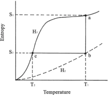
This may be exploited for adiabatic demagnetisation refrigeration (ADR) using the following cycle, illustrated in figure2.4. In the first stage, some quantity of paramagnetic salt is isothermally magnetised by the application of a external magnetic field (shown as the isotherma→bin figure2.4). This represents a reduction in the magnetic entropy and the total entropy of the system. Through this process heat∆Q=T1∆Sis removed from the

system. In practice this is realised by the magetocaloric pill increasing in temperature when it is magnetised. The magnetically generated heat is then removed from the system, allowing it to return to its original temperature.

From this state, the applied magnetic field is adiabatically reduced to zero. As it is an adiabatic process, the total entropy of the system remains constant. The magnetic entropy is increased, requiring that the entropy associated with the system temperature decreases. As a result the system is cooled (the adiabat b→c of figure2.4), to a final temperature T2<T1 and the adiabatic temperature change isTad =T1−T2. Experimentally this step

requires conditions as close to adiabatic as is possible. In contrast to the first where the magnetocaloric must be in good thermal contact with the environment to lose the heat, this requires that the pill and sample stage be thermally decoupled from their surroundings. This change is achieved through a "heat switch", either superconducting, mechanical or gas based.

Materials used for their magnetocaloric properties may thus be evaluated by the compari-son of three parameters particular to the material: the isothermal magnetic entropy change ∆Smag, the adiabatic temperature changeTad and the refrigeration capacity, RC, defined as

RC=

Z T₂

T1

20 Theoretical background

Fig. 2.4 Total entropy of a paramagnetic system as a function of temperature for zero(H1)

and non-zero(H₂)applied magnetic field. Taken from reference [20].

whereT1andT2are the temperatures at the half maximum value either side of the∆S(T)

peak.

These values may be found indirectly through measurements of magnetisation and heat capacity under changing magnetic fields.

Firstly the magnetic entropy change may be found using Maxwell relations as

∆S= Z H₂ H1 ∂M ∂T H dH (2.19)

whereMis magnetisation,T is temperature, subscriptH meaning at constant magnetic field, andH1andH2are the minimum and maximum applied fields. H1is commonly zero

field.

For experimental magnetisation measurement, this is rendered into a more readily appli-cable form by McMichael, Ritter and Shull[21] as

∆SM(Tav) = 1 ∆T Z H 0 M(T+∆T,H)dH− Z H 0 M(T,H)dH (2.20) for two magnetisation isotherms with average temperatureT_av, separated by temperature difference∆T.

This method requires integration of magnetisation curves as a function of field and for the application to real experimental data in the absence of a known equationM(T,H)requires

2.4 The Magnetocaloric Effect 21

some approximation or interpolation. In the absence of interpolation, a trapezoidal method for the calculation of the integrals may be used as proposed by Pecharsky and Gschneidner[22]:

∆S_M(T_av)_∆H= δH 2δT δ M₁+2 n−1

∑

points in field at which magnetisationMis measured, andδH=∆H/(n−1)is the constant

separation in field between these steps.

∆S_M may then be calculated using this method or through fitting and numerical integration of M(T,H) data. In either case the uncertainties arising from these integrations may be minimised by increasing the density of points taken in field (minimisingδH).

Unlike∆S_M, the adiabatic temperature changeT_ad in a magnetocaloric process can not be determined from magnetisation measurements alone. This requires either measurements of heat capacity as a function of temperature and field,C_p(T,H), or measurement heat capacity at zero fieldC_p(T,0)combined with the magnetisation measurements described previously. Both again rely on the effective relation

S(T,H) =

Z T 0

C(T,H)

T dT+S0 (2.22)

whereS₀is the entropy at zero temperature which is usually assumed to be zero. By the calculation of total entropy from heat capacity data, both∆S_M andT_ad may be determined from examination ofS(H,T),S(0,T),T(S,H)andT(S,0)to determined the isotherms and adiabats in figure2.4.

Chapter 3

Methods

The work presented here relied on a number of techniques which may be divided into those performed in the laboratory, principally measurements of magnetic susceptibility, and those reliant on large scale scattering facilities. The advantage of this approach lies in the distinct, complementary physical and material properties which may be explored through these different approaches.

3.1

SQUID Magnetometry

Magnetic measurements of samples were carried out using two Quantum Design Magnetic Property Measurements Systems (QD MPMS). One model MPMS3 (base temperature 1.8 K, maximum field 7 T) and one original MPMS (base temperature 2 K, maximum field 5 T). Both of these systems were used in the DC scan mode and results from both should be directly comparable. The pressure cell set-up detailed in3.4.1is compatible with both systems.

The foundation of this technique is the movement of a sample through the coils of one or more superconducting quantum interference devices (SQUID) and the measurement of the resultant induced voltage. A near-ideal voltage versus position response is shown in figure

3.1.

For most samples, a Levenberg-Marquadt least squares fit to the voltage-position data may be used to calculate the magnetic moment. This fit, as shown in equation3.1, is used by the software supplied with the MPMS[23].

24 Methods -30 -20 -10 0 10 20 30 Position (mm) -0.2 -0.1 0 0.1 0.2 0.3 0.4 Signal (a.u.)

Fig. 3.1 Typical voltage versus position response (red) with Levenberg-Marquadt fit evaluated at each measured position (black).

V(Z) =X₁+X₂·Z+X₃· 2R2+ (Z+X₄)2−32 − R2+ (Λ+ (Z+X4))2 −3₂ − R2+ (−Λ+ (Z+X4))2 −32 (3.1)

whereZ is the sample position,V(Z)is the induced voltage at that position,Xiare free

parameters for fitting, andRandΛare constants: longitudinal radius and longitudinal coil separation of the SQUID respectively.

In this fit X3 is the final parameter of interest, corresponding to a voltage amplitude

which is directly proportional to the measured magnetic moment by factors particular to the instrument used.

The voltage versus position data may also be fitted by the method of singular value decomposition (SVD). This is a linear algebraic technique which has previously seen use for the fitting of small magnetic signals[24].

SVD operates on the assumption that the raw measured voltage (arising from the desired signal and background)V(z)may be treated as an superposition of multipole terms as

3.1 SQUID Magnetometry 25 V(z) = N

∑

where f_i(z)is the voltage signal arising at positionzfrom theith multipole term anda_iis the coefficient of that term. This may equally be expressed in the form

V=Fa (3.3)

whereVis a matrix of lengthMbeing the number of data points in a scan,ais a matrix of lengthN being the maximum multipole term used andF is aM×Nmatrix of which the columns are the values of each multipole term.

The fit is determined by the minimization of the value:

r=|Fa−V| (3.4)

which may be solved through a least squares fitting method to give a solution

afit=V S−1UTV (3.5)

whereU SVT =F is the singular value decomposition of F which may be found by standard matrix algebra.

When the size of the magnetic moment of the sample is similar to or smaller than that of the background from the sample environment, it is necessary to ensure that only contributions to the SQUID voltage from the sample are fitted. Indeed in extreme cases the raw signal may not be possible to fit with the standard methods. In these cases, post-processing of the raw data and background subtraction is required. This is particularly common when using SQUID pressure cells as in3.4.1due to their large mass compared to that of the sample.

The magnetic moment of the sample may be isolated by the repetition of a similar measurement (temperature, field, sample environment) without the sample present. The raw voltage-position data of this background measurement may then be subtracted from the first to recover the response due to the sample which is fit using the methods described previously. This method provides reliable isolation of the desired signal at the cost of the necessary repetition of experiments. For this to be optimally effective, conditions in the sample and background run must be matched as closely as possible. Using the SQUID pressure cell apparatus, this includes matching the effective length of the cell and position of the pistons by loading to matching pressures with only the manometer loaded.

It is accepted that repeated measurements will not perfectly reproduce the desired match-ing steps in both temperature and magnetic field. Usmatch-ing the systems described in this work,

26 Methods

use of the points matching most closely between the two runs in these two parameters is usually sufficient for effective background subtraction, though more advanced techniques involving the interpolation of scans in temperature and field are possible.

With the necessity of high-pressure apparatus used in this series of experiments, a software package was developed in MATLAB alongside collaborators to standardise both the magnetic background subtraction and fitting, to allow for easy comparison of results from LV and SVD fitting. An overview of this work may be found in reference [25].

3.2

Synchrotron X-ray Experiments

To determine of high-pressure crystal structures, x-ray diffraction measurements on the transition metal phosphorus sulphide MPS3 family of materials were carried out at the

Diamond Light Source, Harwell on the beamlines I15 and I19. Experiments on both of these instruments utilised local diamond anvil cell equipment and procedure for high pressure study as detailed in3.4.2.

3.2.1

Powder X-ray Diffraction (PXRD)

High pressure PXRD experiments on Fe, Ni and MnPS3were carried out on I15, the dedicated

extreme conditions beamline at the Diamond Light Source, Didcot, UK.

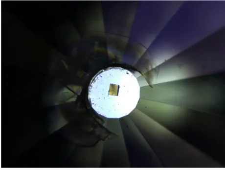
Powder samples of the MPS3 compounds were loaded by Dominik Daisenberger,

in-strument scientist on I15, into diamond anvil cells of culet diameter 400 µm. Pressure was applied via a gas loading membrane system. For comparison of hydrostaticity, measurements were taken both with a helium pressure medium loaded alongside the sample, and without medium, the pressure region being filled completely by the powder sample.

X-rays of wavelength λ =0.4246 Å (E =29.2 keV) were used to collect diffraction

patterns, this being a sufficient energy to pass through the diamond anvils used without significant attenuation. A 2D MAR345 detector was used with collection times varying between 15 s and 45 s.

Raw 2D detector intensity data was processed into a suitable xy format using DAWN

software[26] with LaB6 calibration. Subsequent analysis of powder diffraction data was

carried out using software packages GSAS-II[27] and Topas[28]. Initial solution of unknown high-pressure structures was approached using whole-pattern fitting methods Pawley refine-ment and Le Bail refinerefine-ment. Accurate characterisation of the structures was then carried out by Rietveld refinement. Due to the nature of the experiments, additional parameters were

3.2 Synchrotron X-ray Experiments 27

used in the refinements to account for the effects of pressure on the measured diffraction patterns.

The Rietveld refinement technique fits the measured powder diffraction pattern using both instrumental and sample characteristics as fitting parameters to minimise the function:

M=

_∑

σ_i2

(yi−yci)2 (3.6)

whereσiis the variance of the observationyi,yiis the observed intensity at positioni

andyciis the calculated intensity at positioni. The calculated intensity is determined by a

number of contributing factors as

y_ci=y_bi+ Phases

∑

∑

wherey_bi is the background intensity at position i; S_n is the scale factor for phase n, proportional to its volume fraction; j_k is the multiplicity of the kth reflection; L is the Lorentz factor;Ois a factor describing the effects of preferred orientations, or the departure from a purely random orientation distribution; |F| is the structure factor; Ω is the peak profile function, approximating broadening effects from instrument and sample. The second summation runs over all reflectionsk₁tok₂contributing at positioni[29]. MeasuredMPS3

materials were assumed to be a single pure phase of the desired compound free from impurities.

Expected peak positions from the diamond anvils were calculated, and features at these positions excluded from analysis of the sample diffraction. These positions were calculated using the known incident wavelength and the cubic space-group of diamond inFd¯3mwith a lattice parametera=3.566 61 Å. The unavoidable overlap of sample peaks with diamond peaks intrinsic to the experimental setup means that sample peaks falling at the same angle as those from diamond are unusable for, and excluded from, analysis.

Preferred orientations in the measuredMPS3materials may affect the relative intensities

of diffraction peaks such that they do not fit predictions based on the basic structure. Spherical harmonics were used as free parameters in the fits for the measured diffraction patterns to correct for this. This correction to the peak intensity isA(h,y), given by

A(h,y) =1+ L

∑

∑

∑

28 Methods

wherelis harmonic order up to the maximum usedL. The harmonic termskm_l (h)and kn_l(y) take values determined by the crystal and sample symmetry respectively and the coefficientsC_lmn are refined[30].

The magnitude of the texture is given by the texture indexJ[31]:

J=1+ L

∑

∑

∑

J is equal to unity for a truly random material, increasing for textured samples, and becoming infinite for single-crystal data[32].

Strain in the measured material as is expected in high-pressure experiments also has the effect of changing the peak shapes seen in the diffraction pattern. The effects of strain include both peak broadening and asymmetry[33]. This is accounted for similarly in GSAS-II and Topaz. Peak broadening is also expected to be inversely proportional to crystallite size in the sample by the Scherrer equation:

∆(2θ) = Kλ

τcosθ. (3.10)

where∆(2θ)is the line broadening at FWHM,Kis a dimensionless shape factor with 0.9

being a good estimate in the absence of specific shape information,λ is the x-ray wavelength

and τ is the mean crystallite size. This is most applicable to crystallite of size less than ∼0.2 µm.

Structureless solutions using the method of Pawley refinement are carried out in a similar fashion with the significant caveat that the intensity of theith reflection is no longer determined by factors such as atomic species or position, but is instead a free parameter which may be varied. In this way, the relevant factors which are determined for the structure are the space group and unit cell dimensions. This may still be combined with other considerations such as spherical harmonics to account for preferred orientations to fit the observed pattern.

3.2.2

Single Crystal X-ray Diffraction

Complementary to PXRD, single crystal x-ray diffraction experiments were used to aid in structure determination ofMPS3compounds. These experiments were performed at Diamond

on the I19-2 "Small Molecule Single Crystal Diffraction" beamline. A similar pressure set-up as described for powder x-ray diffraction was used.

X-rays of wavelength 0.4589 Å (E=27 keV) were used to collect the diffraction patterns with a Dectris area detector. Diffraction from the sample is easily separated from that arising from the gasket, due to the latter’s amorphous nature giving rings of diffraction as opposed to

3.3 Neutron Scattering 29

sharp spots. Scattering from the diamond anvils requires more consideration but is generally recognised by it being far more intense than the sample peaks due to the greater volume from which diffraction occurs.

Analysis of single crystal diffraction data was performed using Agilent CrysAlis Pro software with specifications provided by the I19 beamline scientists. Firstly the gasket rings were masked and excluded from peak searches. The UB orientation matrices for the two diamond anvils were obtained by searching found peaks for the known cubic cell of diamond which was assumed to be static with pressure. Peaks found to be corresponding to the diamonds were removed for the subsequent analysis. From the remaining peaks not attributed to the diamond or gasket rings, CrysAlis Pro was used to fit a unit cell and to integrate the diffraction patterns. Once a suitable unit cell was determined by fitting using Cryslalis Pro, the structure was refined to determine atomic positions using SHELX[34] within the WinGX package[35].

The opening angle of the diamond anvil cells used for this single crystal experiment was 28° which, depending on the orientation of the sample, further limited the accessible regions in reciprocal space in one direction. For the platelet crystals of theMPS3compounds,

the accessible region of reciprocal space is limited along thec∗direction. This limits the information from which relevant lattice parameters may be derived.

3.3

Neutron Scattering

Complementary to x-ray scattering methods, elastic neutron scattering was used to study the MPS3materials. Neutron diffraction allows for the direct measurement of not only the atomic

structure which can be examined with x-rays, but also the magnetic structure of systems containing non-zero magnetic moments. The main use of neutron scattering techniques for this work is this magnetic structure determination, as the greater intensity of x-ray scattering allows for more accurate and precise analysis of the underlying crystal structures.

3.3.1

Powder Neutron Diffraction

Powder neutron diffraction was used to study the high pressure magnetic structure of FePS3.

Experiments were carried out on the D20 beamline at the ILL, Grenoble.

Neutrons of wavelength 2.42 Å (E = 13.97 meV) were selected through a graphite monochromator.

30 Methods

The scattering of neutrons by a target within the Born approximation may be characterised by the differential cross-section for a neutron with incident wave vectorkiand spinσiand a

final state withkf andσf as follows:

dσ dΩ(kfσf,kiσi) = m 2π_ℏ2 2 <k_fσ_f|V(r)|k_iσ_i> 2 (3.11) whereV(r)is the potential experienced by a neutron at distancerfrom the scatterer and mis the neutron’s mass. For elastic scattering whereink_f

=|ki|the scattering vector may

be defined asQ=ki−kf .

Due to the non-zero magnetic moment the neutron, scattering occurs by two separate mechanisms. Nucleon-nucleon scattering from sample nuclei is effectively isotropic due to the range of the relevant interaction being much shorter than the wavelength of thermal neutrons. Additional scattering arises from coupling of the neutron spin with magnetic fields arising from unpaired electrons in magnetic materials. For an incident beam of unpolarised neutrons, interference between nuclear and magnetic scattering does not occur, and the differential cross section may be simply broken up into nuclear and magnetic components as

dσ dΩ(Q) = dσN dΩ (Q) + dσM dΩ (Q) (3.12)

In an identical manner to powder x-ray diffraction methods, intensity is measured as a function of scattering angle 2θ from which scattering as a function ofQ= 2_dπ may be derived

by Bragg’s law.

nλ =2dsinθ (3.13)

whereλ is the neutron wavelength used,d is the plane spacing.

The separation of magnetic scattering from that arising from the crystal structure may be achieved in a number of ways. Spin-polarised measurements may be performed which can differentiate between scattering from spin-flip and non-spin-flip processes. In the simpler case utilised here, this is achieved by measurements at temperatures above and below expected magnetic transitions. Peaks appearing only at temperatures belowT_c can be attributed to magnetic effects as long as there is no simultaneous structural transition. Similarly, for a known crystal structure, Bragg peaks at d-spacing values corresponding to non-integer values of(hkl)are due to the magnetic ordering vectorkM in the absence of incommensurate

crystal structures. Magnetic Bragg peaks may also appear at integer(hkl)values which are forbidden for the space group of the underlying crystal structure.

For the case of kM = 0 magnetic ordering, no additional peaks will be seen in the

3.4 High Pressure Methods 31

to an existing structural Bragg position. SuchkM =0 can correspond to a ferromagnetic

structure, colinear antiferromagnetism or non-colinear structures depending on the underlying crystal space group. In this case it is only the intensities of the different magnetic peaks which can be used to distinguish between the possible magnetic configurations[36].

Where performed, structural solution and refinement is carried out in much the same way as for results of powder x-ray diffraction experiments.

3.4

High Pressure Methods

The methods used in this work to achieve high pressures can broadly be grouped into two categories: piston cylinder cells, and anvil cells. Within each of these classes, multiple designs of pressure cell may be used depending on the target pressure and the requirements of the measurement to be performed, being for example a low magnetic background or transparency to x-rays or neutrons.

3.4.1

SQUID Piston Cylinder Cell

For high-pressure SQUID magnetometry measurements, a miniature piston cylinder cell manufactured by CamCool was used. In this type of clamp cell, pressure is attained by the compression of a liquid pressure medium containing the sample and necessary wiring or manometer etc. This type of pressure cell has the advantage of a large sample volume compared to anvil-type cells (up to the order of 1–10 cm3), with the drawback of a lower maximum pressure without making the cell apparatus prohibitively large. To allow for electrical measurement, such as four-point resistivity or capacitance measurements, wiring may be introduced to the pressure region through a feedthrough sealed with a rigid epoxy plug without compromising the attainable pressure in the cell, though for this study this type of cell was used only for contactless magnetisation measurements.

A disassembled cell is shown in figure3.2. This 8.6 mm outer diameter of this cell is such that it can fit entirely within the SQUID coils in a commercial magnetometer, including those discussed in3.1. To minimise the magnetic background from this cell inside the SQUID, the body is made from beryllium copper (BeCu). The combination of small diameter and the relatively soft alloy body limits the maximum pressure attainable in this cell to approximately 1.2 GPa, which is reached by an applied load of∼6 kN.

The sample is loaded into a polytetrafluoroethylene (PTFE) cap of inner (outer) diameter 1.4 mm (2.5 mm) filled with a liquid pressure medium. Most commonly used in this study was Daphne 7373, a mixture of olefins commonly used in high pressure studies. Daphne 7373

32 Methods

Fig. 3.2 CamCool manufactured SQUID piston cylinder cell. The outer diameter of the cell body is 8.6 mm, with the PTFE cap enclosing the sample space having an inner diameter of 1.4 mm. (Bottom) exploded view: (a) bottom lock nut, (b) bottom piston, copper ring, and PTFE cap assembly, (c) cell body, (d) anti-extrusion disk, (e) inner piston, (f) top lock nut.

solidifies at 2.2 GPa at room temperature[37] and exhibits almost no discontinuous pressure drop on solidification[38]. At pressures of up to 1 GPa, Daphne 7373 freezes at∼200 K. The pressure loss on cooling from 300 K to 4.2 K using similar apparatus as described here has been measured to be 0.15–0.17 GPa irrespective of the initial pressure[38].

Prior to the loading of the measurement sample, a small sample of lead is loaded to function as a manometer. This lead is sized such that it does not block the PTFE cap, and the assumption is made that both the sample and the manometer are free to move under gravity inside the liquid medium, and lie in contact. Care must be taken when loading the manometer and sample that air bubbles are not trapped in the pressure medium, as this may cause the cap to fail under load due to uneven forces inside the pressure region. For the same reason the cap is filled with a slight excess of pressure medium such that air is not trapped inside when the cell is assembled in the next step.

With the sample and manometer submerged in the pressure medium inside the PTFE cap, the lower piston is inserted into the open end of the cap, with the copper ring around the piston. This copper ring is soft and is designed to deform first to seal the pressure medium and prevent the extrusion of the PTFE cap under load. This assembly is inserted into the cell body and pushed into position under a loading force of 2 kN to overcome friction between the cap and the cell bore and to ensure it is firmly in contact with the cell body. The bottom lock nut is then screwed in by hand, and gently tightened using a small spanner. At the blank end of the PTFE cap, accessed through the other end of the cell body, the anti-extrusion disk is inserted into the cell bore for the same reason as the copper ring around the lower piston. The inner piston follows this around which the top lock nut is screwed on. The loading force is applied using a hydraulic press, through the external piston pushing on the inner piston. Once the desired loading force is applied, the pressure is locked in place by tightening the

3.4 High Pressure Methods 33 2 2.5 3 3.5 4 4.5 5 5.5 6 6.5 Load (kN) 0.2 0.3 0.4 0.5 0.6 0.7 0.8 0.9 1 1.1 1.2 Pressure (GPa)

Fig. 3.3 Pressure inside the sample space of the SQUID piston cylinder cell, determined from lead mangetisation measurement and equation3.14, against applied cell load. The uncertainty is dominated by the intrinsic width in temperatures of the superconducting transition.

top lock nut against the inner piston. An experimentally determined pressure-load relation and pressure cell length relation are shown in figure3.3.

Sample alignment may be roughly controlled through the relative dimensions to which it is cut relative to the the known crystallographic orientation. Ideal samples are cut in a needle geometry such that possible rotation about the short axes is limited by the inner diameter of the PTFE cap. This sample geometry simultaneously helps to minimise the demagnetising field generated.

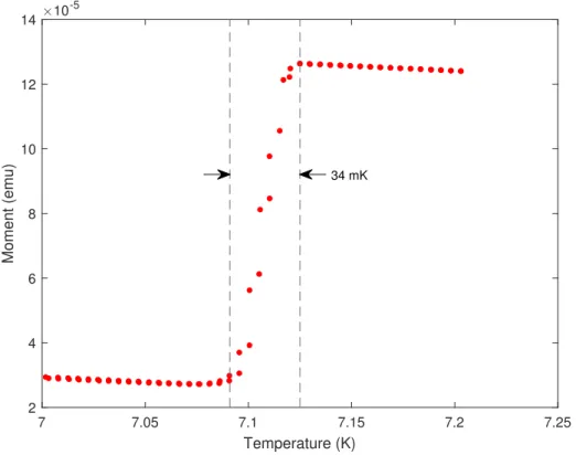
Pressure is determined from the lead manometer by the measurement of its superconduct-ing transition temperature,T_caccording to reference [39] by:

T_c(P) =T_c(0)−(0.365±0.003)P (3.14) whereT_cis measured in K andPin GPa. This relation holds for pressures up to 5 GPa, well above the maximum pressure attainable in this cell.

Uncertainty in the measured pressure arises from uncertainty in the measured supercon-ducting transition temperature. In contactless magnetisation measurements, this is dominated by the intrinsic width of the superconducting transition rather than uncertainty in the

temper-34 Methods 7 7.05 7.1 7.15 7.2 7.25 Temperature (K) 2 4 6 8 10 12 14 Moment (emu) 10-5 34 mK

Fig. 3.4 Magnetisation measurement of the superconducting transition of lead in SQUID pressure cell loaded with 2.5 kN force corresponding to a pressure of 0.26(4)GPa.

ature measurement in the systems used. An example magnetisation measurement of the lead superconducting transition is shown in figure3.4.

3.4.2

Diamond Anvil Cell

For pressures above those achievable with piston cylinder type pressure cells, diamond anvil cells (DAC) may be used to perform similar experiments. Wired measurements of resistivity or AC susceptibility are achievable but for the results presented here the use of DACs is limited to contactless measurements by x-ray and neutron methods.

The pressure region in these cells is enclosed by the culets of the diamonds and the metallic gasket through which a hole of diameter less than half that of the culets has been drilled (the culets are only approximately circular and thus the diameter is an average). The volume of this pressure region is as a result orders of magnitude reduced compared to PCCs. A liquid pressure medium may be used to maintain hydrostaticity up to pressures on the order of 10 GPa.

Pressure determination inside DACs was achieved using two methods. For x-ray exper-iments, spheres of ruby smaller than the sample (∼10 µm diameter) were inserted in the