A Multivariate Test For Similarity of Two Dissolution Profiles

A Multivariate Test For Similarity of Two

Dissolution Profiles

H. Saranadasa and K. Krishnamoorthy 1* 2

1 Ortho McNeil Pharmaceutical, Inc., Raritan, New Jersey, USA 2 University of Louisiana at Lafayette, Lafayette, Louisiana, USA

ABSTRACT

A multivariate test of size α for assessing the similarity of two dissolution profiles is proposed. The inferential procedure is developed using the approach for the common mean problem in a multivariate setup due to Halperin (15). The performance of the proposed method is compared with Intersection Union Test as well as criterion recommended by the FDA through a simulation study. All the methods are illustrated using real examples.

2

f

Key words: Profile similarity; f2 factor; Student’s t variable; Size α test; Intersection Union Test; Common mean.

1. Introduction

Dissolution testing is performed on 6 or 12 dosage units (assume tablets or capsules are the dosage form) and placing them in agitated media. The dissolution test system has six vessels, each holding a liter of media. A rotating basket or paddle is lowered to agitate the contents, after which a tablet is dropped into the vessel and dissolution samples are collected at different time points (for example every 15 min in first hour and every 60 min after the first hour) and analyzed, usually via chromatography or UV spectroscopy. The response at time t is the cumulative amount (%) of drug released into the media. The dissolution profiles for solid dosage forms are developed in connection with observations taken on tablets or capsules, over time. It is the curve of the mean dissolution rate (cumulative % dissolved) over time. The pharmaceutical scientists are

*Correspondence: Hewa Saranadasa, Pharmaceutical Sourcing Group Americas, A Division of Ortho McNeil Pharmaceutical, Inc. Johnson & Johnson Company, 1000 Route 202, P.O.Box 300, Raritan, NJ 08869-0602; E-mail: [email protected].

interested in a comparision of these profiles under different conditions related to formulation forms, lot-to-lot and brand-to-brand variation. For example, if dissolution profile similarity is demonstrated between the prechange drug product and the postchange formulation, in vivo bioequivalence testing can be waived for most changes. It is a big advantage for the industry to avoid conducting clinical studies to demonstrate bioequivalency and these studies are not only time consuming, but also expensive. For some drugs, bioavailability needs to be demonstrated only if the product fails to achieve adequate dissolution when compared to a test standard. Also in the manufacturing phase, dissolution profile of a new lot (may be some changes with respect to chemical manufacturing and control) will be tested against the validation lots for similar dissolution profiles to assure the compliance. Therefore, it is of great interest to the pharmaceutical scientist to compare dissolution profiles. The statistical challenge is that how to define and test the two population dissolution profiles are “similar” based on the sample dissolution data collected over time.

The U.S. Food and Drug Administration (FDA) has issued several guidelines describing circumstances for which Scale Up and Post Approval-Change ( SUPAC) in the components of drug product manufacturing site or the manufacturing process and equipment of formulation are acceptable. One requirement is to establish the similarity of dissolution across a suitable time interval.

The U.S. FDA’s guidance for industry on dissolution testing of immediate-release (IR) solid oral dose forms (1) as well as SUPAC-IR (2), SUPAC-MR (3), and Bioavailability and Bioequivalence study guidance for oral dosage forms, describes the model independent mathematical approach proposed by Moore and Flanner (4) for calculating a dissimilarity factor ( ) and a similarity factor ( ) of dissolution across a suitable time interval. The similarity factor (where 0

1

f f₂

2

f ≤ f2 ≤100 and 50%

implies dissolution profiles are similar) is a function of mean differences and does not take into account the differences in dissolution within the test and reference batches.

2

Hence careful interpretation is warranted when is used as a similarity factor when the variances of the profiles are very different.

2

f

Previous articles have discussed the more serious deficiencies of using the factor for assessing the similarity between two profiles. One of the major drawbacks identified was finding the sampling distribution of the statistics. This statistic has complicated properties and deriving the distribution of the statistic is not mathematically tractable. Shah et al. (5) proposed a bootstrap method to calculate a confidence interval for the factor. Because is sensitive to the measurements obtained after either the test or reference batch has dissolved more than 85%, Shah et al. (5) recommended a limit of one sampling time point after 85% dissolution. A recent paper, discussing the aspects of the dissolution profile testing problem, by Eaton et al. (6) also raised some issues concerning the use of the statistic.

2 f 2 f 2 f 2 f

Several other authors discussed criteria for statistical evaluation of similarity of dissolution profiles using model-independent as well as model-dependent approaches. Some of the model-dependent approaches were discussed by Sathe et al. (7). Tsong et al. (8) and Chow et al. (9) proposed methods based on autoregressive time series models. Wang et al. (10) showed that the methods using (a) Intersection Union Test (IUT) (b) the Likelihood Ratio Test (LRT) and (c) inversion of the Hotelling’s

2

T confidence region are all equivalent. The hypothesis testing procedures are based on

criterion and resampling by bootstrap method has been discussed by Shah et al. (5) and Ma et al. (11,12).

2

f

In the FDA guideline for industry, the procedure allows the use of mean data and recommends that the Relative Standard Deviation (RSD) at an earlier time point (for example 5 or 10 minutes) not be more than 20%, and at other time points not more than 10%. In instances where the RSD within a batch is more than 15%, the guideline

suggests using a multivariate model-independent procedure, but no references are given for these situations.

The methods proposed by Tsong (13) and Saranadasa (14) are based on confidence set method using a multivariate normal distribution. In this article, we consider Saranadasa (14) proposal and give an exact solution for establishing similarity of dissolution profiles. Saranadasa (14) approach will be briefly discussed at the end of Section 4. The solution is based on our observation that the present problem, in the setup of Tsong (13) and Saranadasa (14), is equivalent to the hypothesis testing problem for the common mean of a multivariate normal distribution discussed by Halperin (15) and Krishnamoorthy and Lu (16).

Let us first introduce some notations to understand the two multivariate tests proposed in the literature and which will be presented in next two sections.

Let be the observed cumulative percent dissolved for dosage unit j at sampling time for formulation

i

, where

i

=1, 2 (1: Reference formulation and 2: Test formulation), j=1,2,…, and k=1,2,…, p (p time points). Let

ijk

u

k

t

i

n

u1 and u2denote the

sample mean vectors of the reference profile and test profile respectively. Let is the absolute mean difference at time point. Then

|

|

d

_k

k

t

ud = −u1 u2 =(ud1,…,udp)' is the sample mean difference vector and the corresponding population vector is defined as

µ

=

µ

₁

−

µ

₂. The problem of interest is to test the hypotheses

0: i 0 or i 0 for some vs. a : 0 i 0 for all , (1.1)

H µ δ> µ < −δ i H −δ ≤µ δ≤ i

where δ0 is the pre-specified acceptable dissolution profile difference. To establish the similarity of dissolution across a suitable time interval, the value of δ0 = 10.

2. The Fit Factor

f2

The FDA promoting fit factor, is a mathematical index (0f2 ≤ 100) constructed by a function of Euclidean distance of population dissolution mean difference vectors of test and reference formulations. As defined earlier,

2

f ≤

2

1

µ

µ

µ

=

−

(µ1 and µ2 are the population mean vectors of length p of reference and test formulation respectively). The is defined by Moore and Flanner (4) as follows: f2

f₂ =50 log₁₀ 1 2 ' 100 1 . p µ µ − ⎛ ⎞ ⎛ ⎞ ⎜ ₊ ⎜ ⎟ ⎜ _{⎝ ⎠} ⎜ ⎟ ⎝ ⎠ ⎟ ⎟ (2.1)

Notice that f₂ =100 when the two dissolution profiles are identical (i.e. µ'µ =0). If the dissolution of one formulation is completed (100%) before the other begins, then

log 50 2 = f 10

(

)

2

)

1 2 100 1 ( 100 + − = -0.001 ~ 0. If |µ1i −µ2i | = 10 for all ,

is very close to 50 and dissolution profiles with

p

i=1,2,..., f2 |µ1i −µ2i | 10 (or

50%) for all are considered as similar dissolution profiles according to the FDA guideline (1).

≤

2

f

≥

i=1,2,...,p

3. Intersection Union Test (IUT)

As we mentioned in the earlier section (see Wang et al. (10) for more details), the Intersection Union principal leads to a test of the form: Reject dissimilar dissolution profiles if 1/ 2 2 0 | | k dk s u c n δ ⎛ ⎞ + ⎜ ⎟

⎝ ⎠ < for all time points , where

t

k |udk|is the observed absolute mean difference at the th time point,

t

_k

δ

₀ is the pre-specified acceptable dissolution profile difference, is the pooled variance of the two dissolution profiles at the th time point, n is the degrees of freedom (

2 k

s

k

percentile of the Student’s t distribution with n degrees of freedom. Berger and Hsu (17) showed that this is a size α test.

4. The Proposed Multivariate Approach

Suppose uij~Np(µi,Σ), j=1,2,...ni and i=1, 2, are two independent multivariate normal dissolution profiles, one being a reference batch or a pre-change batch and other being a test batch or post-change batch. Samples were taken at pdifferent common

time points; ’s are the number of tablets used in reference and test batches, normally and the common sample size is 6 or 12. Let

i

n

2

1 n

n = u₁ and u₂denote the sample mean

vectors of the reference profile and test profile respectively; let and denote the sample variance-covariance matrices of the reference profile and test profile respectively. Then 1 S S₂

∑

= = ni j ij i i u n u 1 1 and

∑

=

−

−

−

=

ni j i ij i ij i i

u

u

u

u

n

S

1

)'

)(

(

1

1

, i=1,2.

To establish similar dissolution profiles, let us assume that µ µ₁− ₂ =e ,δ where e denotes the px 1 vector of ones, and δ is an unknown constant. This implies that the

sample mean difference vector,ud =u1−u2, of two profiles,

d u ~

_⎟⎟

⎠

⎞

⎜⎜

⎝

⎛

Σ

⎟⎟

⎠

⎞

⎜⎜

⎝

⎛

+

2 1

1

1

,

e

n

n

N

_p

δ

independently of V =(n1+n2 −2)S =(n1 −1)S1+(n2 −1)S2~Wp(n1+n2 −2,Σ), where

denotes the Wishart distribution with degrees of freedom n and the scale matrix ∆. We here note that S is an unbiased estimator of

) , (n ∆ p W Σ.

Notice that, to establish similar dissolution profiles, it is enough to find sample evidence in favor of H_a:− ≤ ≤δ₀ δ δ₀. Thus, we want to test

0: 0 or 0 vs. a: 0 .

H δ δ> δ < −δ H −δ ≤ ≤δ δ₀ (4.1)

We like to pint out that whenever in (4.1) holds, then the in (1.1) also holds. The above hypothesis testing problem is a two-sample version of the one-sample “common mean” problem considered by Halperin (15) and recently by Krishnamoorthy and Lu (16). In the one-sample case, we have a multivariate normal population with mean vector

a

H H_a

e

µ= δand unknown covariance matrix Σ, and the problem of interest is to develop inferential procedures about δ based on a sample of observations. Therefore, solutions to the present problem can be easily obtained from the results of the papers just cited.

If Σ is known, then the best linear unbiased estimator for δ is given by

1 1

e 'Σ−u_d /(e 'Σ−e). If is unknown, then replacing it by the sample covariance matrix

S, we get the following natural estimator Σ ˆ e ' 1₁ e ' 1 e ' e e ' e d S u V u S V δ = −₋ = −₁d − (4.2)

of δ, which is also the maximum likelihood estimator. As pointed out by Halperin (15), the following transformation is useful to describe the distribution of . Let δˆ

1 d

u

y= , x1 =ud1−ud2, …,xp−1 =ud1−udp,

where u_di denotes the ith component of u_d. In matrix notation, we write this

⎟⎟ ⎠ ⎞ ⎜⎜ ⎝ ⎛ X y =Aud, where , ⎟ ⎟ ⎟ ⎟ ⎟ ⎟ ⎠ ⎞ ⎜ ⎜ ⎜ ⎜ ⎜ ⎜ ⎝ ⎛ − − − = 1 ... 0 0 1 ... ... ... ... ... 0 ... 1 0 1 0 ... 0 1 1 0 ... 0 0 1 pxp A Write ⎟⎟ ⎠ ⎞ ⎜⎜ ⎝ ⎛ = 22 21 11 0 A a a A and _⎟⎟ ⎠ ⎞ ⎜⎜ ⎝ ⎛ = 22 21 12 11 V v v v V

so thata₁₁ and v₁₁ are scalars and

say. , ' ' ' ' ' 22 22 22 22 12 12 12 21 22 21 11 21 11 21 22 11 11 21 22 12 11 21 11 11 11 ⎟⎟ ⎠ ⎞ ⎜⎜ ⎝ ⎛ = ⎟⎟ ⎠ ⎞ ⎜⎜ ⎝ ⎛ + + + + + = XX Xy yX yy W w w w A V A A v a a v A a v a a v A a v a A v a a v a v AVA

In terms of these notations, we can write asδˆ X W w y yX XX 1 ˆ_{= −} − δ . Let X W X n n Q XX 1 1 2 1 ' 1 1 − − ⎟⎟ ⎠ ⎞ ⎜⎜ ⎝ ⎛ + = . Then, Q ~ 1, , 2 1 2 1 1 p n n p F p n n p − + − − + −

where Fa,b denotes the F random variable with the numerator degrees of freedom a and the denominator degrees of freedom b. It follows from Halperin (15) that, conditionally given Q,

. 1 1 ) 1 ( , ~ ˆ 2 1 yy.X ⎟⎟ ⎠ ⎞ ⎜⎜ ⎝ ⎛ ⎟⎟ ⎠ ⎞ ⎜⎜ ⎝ ⎛ + + n n Q N δ σ δ Furthermore,

1 ˆ 2 1 1 . − − + − = − p n n w W w w_{yy yX XX Xy} X yy σ ~ 2 1 2 1 . 2 1 1 + − − − − + n n p X yy p n n χ σ

independently of Q. Therefore, conditionally given Q, the pivotal quantity

(

)

) 1 ( ˆ ) ˆ ( / 1 / 1 . 2 1 2 1 Q n n T X yy + − + = − σ δ δ _{~ , (4.3)} 1 2 1+n −p− n t

where tm denotes the Student’s t variable with degrees of freedom m.

Notice that if samples of data provide evidence against in (4.1), then we conclude that the dissolution profiles are similar. The

0

H

0

δ

is 10% equivalent to the 50% critical value recommended in the FDA guideline for the criterion. It is clear from the distribution of

2

f

ˆ

δ and (4.3) that our problem is essentially testing if a normal mean is contained in a known interval, which has been well addressed in assessing the average bioequivalence of two drugs. A standard approach for the latter problem is due to Shuirmann (18, 19). This approach is known as two one-sided tests (TOST), and using this approach we reject the above null hypothesis when

1 2 1 2 0 0 1,1 1,1 ˆ ˆ and , n n p n n p t t SE α SE α δ δ δ δ + − − − + − − − + _> − _{< −} where . ) / 1 / 1 )( 1 ( ˆ _. Q n₁ n₂ SE = σ_yyX + +

In other words, the null hypothesis in (4.1) will be rejected if the (1 - 2α) confidence

interval is contained in the interval

1 2 1,1

ˆ _{( )}

n n p

t _α

δ ± _{− − − −} SE (−δ δ₀, ₀). Even though the confidence level is (1 - 2α), the type I error rates of the above test are always less than or equal to the nominal level α. For more about the Shuirmann’s approach, its properties and other tests for average bioequivalence problem, we refer to Berger and Hsu (17) and Chow and Liu (20). If one wants to use the p-value approach, then the null hypothesis in (4.1) will be rejected if 1 2 1 2 0 0 1 1 2 1 ˆ ˆ and n n p n n p P P t P P t SE SE δ δ _α δ δ _α + − − + − − ⎛ + ⎞ ⎛ − = ⎜_⎜ > ⎟_⎟< = ⎜_⎜ < ⎝ ⎠ ⎝ ⎞ < ⎟⎟ ⎠

or

p-value = max

{

P₁,P₂

}

<α.

Remarks:

(1) Halperin also proposed an unconditional test for the problem considered in his paper. This unconditional test for our present problem is based on the pivotal

quantity

(

n n

)

yy.X 1 2 1 1/ (ˆ )]/ ˆ / 1 [ + − δ −δ σ which is distributed as =

. Krishnamoorthy and Lu’s (16) numerical method can be readily used to compute the exact percentile points of for a given , , p and q t 2 / 1 1(1 ) 2 1 Q tn+n −p− + q t n₁ n₂

α . However, their power comparison studies for the one-sample case showed that the conditional test is slightly more powerful than the unconditional test. Because the conditional test is not only simple to use but also it is more powerful than the unconditional test, we recommend only the conditional test for practical applications.

(2) The procedure suggested by Saranadasa (14) is based on the (1-α)×100% confidence region for the mean difference vector of the two profiles and assume that the population difference mean vector is of the form

e

δ , where e denote thepx 1 vector of ones. Based on the same assumptions considered in

this paper, one looks at the set of δ such that:

C e d u S d u −

e

)' −1( − ) ≤ ( δ δ , where 1 2 1 2 ( ) ( ) , 1 1 p n n n C F_{p n p} n n _{n p} α + = _{− +} − + , and n=n1+n2−2 .

A solution for finding the maximum δ satisfies the above inequality was presented in Saranadasa (14) and it was used to establish the similarity of two dissolution profiles. In contrast to the above approach, in this paper we developed a statistical test for testing hypotheses (4.1) for given specification ofδ .

5. Practical Applications

The performance of the proposed procedure was compared with the criterion on real data examples. Two groups of three pair dissolution profiles were used. The first group consists of similar dissolution profiles (same formulation of two marketed lots) and the second group includes different dissolution profiles of two dosage strengths. The results are summarized in Tables 1 and 2:

2

f

[Insert Tables 1 & 2 here]

[Insert Figures 1.1 and 1.2 here]

In practice the threshold value for criterion is allowed as 50% in order to declare similar dissolution profiles according to the FDA guideline (1). The corresponding mean difference at each time point would not be more than 10%. Therefore, we use 10% mean difference for testing the proposed multivariate test with 5%

2

f

α -level, 10% mean difference for IUT test with 5% α -level and 50% threshold for f2 criterion.

Table 1 summarizes the results of 3 tests for the application of the 3 similar dissolution profiles. The proposed test correctly classified the all 3 pair profiles as similar while criterion misclassified one example (Figure 1.1A) as dissimilar profiles. The IUT failed to classify none of the examples as similar profiles even though there were similar.

2

f

Table 2 summarizes the classification results of 3 dissimilar profiles. All three criteria correctly discriminated all profiles as different dissolution profiles.

6. A Simulation Study

We carried out a simulation experiment to examine the performance of , Intersection Union test (IUT) and the proposed multivariate test. The multivariate random samples

2

of size 12 were generated from a multivariate normal distribution. The mean vectors for the two profiles were chosen at 5, 10, 15 and 20 minutes following an S-Shape logistic dissolution model of the form:

_{( )} ) ( 50 50 1 bt t t t b t e e Q y _{− −} − − + =

with the variance-covariance structure (Σ) of the form:

, 2 4 3 4 43 2 4 42 1 4 41 4 3 34 2 3 2 3 32 1 3 31 4 2 24 3 2 23 2 2 1 2 21 4 1 14 3 1 13 2 1 12 2 1 ⎟⎟ ⎟ ⎟ ⎟ ⎠ ⎞ ⎜⎜ ⎜ ⎜ ⎜ ⎝ ⎛ = Σ σ σ σ ρ σ σ ρ σ σ ρ σ σ ρ σ σ σ ρ σ σ ρ σ σ ρ σ σ ρ σ σ σ ρ σ σ ρ σ σ ρ σ σ ρ σ

where σi is the standard deviation of dissolution values at ith time point (i = 5, 10, 15 and 20 min) and ρij is the correlation coefficient of ijth time point. We chosen the variance-covariance parameters, which would mimic the nature of the variability of the typical dissolution experiments. The model parameters and variance-covariance parameters are given for two cases below:

Case (1) Q=90.4, b=−.36, t₅₀ =6.8 (time taken to dissolve 50%)

σ₁ =8, σ₂ =3, σ₃ =2, σ₄ =2 and RSD’s are 25.8%, 4.4%, 2.3% and

2.2% at each time point

ρij =0, .3, .5 and .7 for all i,j.

Case (2) Q=90.4, b=−.36, t₅₀ =6.8(time taken to dissolve 50%)

σ₁ =3, σ₂ =3, σ₃ =2, σ₄ =2 and RSD’s are 9.7%, 4.4%, 2.3% and

2.2% at each time point

ρij =0, .3, .5 and .7 for all i,j.

One thousand experiments for each configuration were simulated from the respective multivariate normal distribution. The numbers of experiments failing the null hypothesis (i.e. H_a :similar dissolution) by each of three criteria were counted. The

experiments were repeated for mean shift of 0, 2, 4, 6, 8, 9.5, 10, 10.5, 12 and 15% between the two profiles. The results are summarized in Tables 3-4:

Tables 3 & 4 are here

7. Concluding Comments

In this article we proposed a multivariate procedure for the case where it is reasonable to make the assumption of multivariate normality of the data. The proposed method was compared with the Intersection Union test as well as criterion recommended by the FDA guideline. A simulation study was conducted to compare the 3 procedures for the same data. The results showed that test and the proposed test have almost same power when 2 f 2 f % 6 ≤

δ , but test is at the cost of a highly inflated Type I error at the selected mean difference of dissolution profiles that are considered to be similar. This error rate is in general more than 45% on average at 10% mean difference. That is test tends to accept different dissolution profiles as similar dissolution profiles with more that 45% of the time at the selected mean difference of dissolution profiles ( 2 f 2 f %) 10 =

δ . However, proposed test maintains the Type I error rate at the selected α -level at the pre specifiedprofile difference that is considered to be acceptable (10%).

The Intersection Union test showed lower power compared to both and proposed test when the data variability was considerably high (see case 1). In general the type I error rates for IUT were under

2

f

α -level for the most cases.

Due to the inclusion of several time points after the effective completion of dissolution (>85%) the criterion as well as the proposed criterion tends to produce significant results in favor of similarity. Therefore, we also recommend limiting one sampling time point after 85% dissolved for using the proposed criterion (see (1) for using ). As is seen in the example 1.1A, the criterion and the proposed criterion lead two different conclusions for this case study. The data showed that at 2 minutes tablet-to-tablet variability was very high (RSD >20%), the observed mean difference was as high as 22% compared to the rest of the time points and low power (68%)of estimating mean difference within 10% with observed high variability with 6 tablets. Since the criterion does not consider tablet-to-tablet variability at each time point (not formulation related) into the calculation of score, it concludes dissimilar dissolution profile solely on 2 minutes time point difference. On the other hand, the proposed test statistic of the procedure is based on an estimator, which is a weighted average of the mean profile differences at all time points and the weights are based on the inverse of the estimated variance at each time point. It is reasonable to weight the mean difference by their variance because the variability at each time point is not mostly formulation

related but it is due to inherent dissolution method variability. 2 f 2 f 2 f 2 f 2 f

References

1. US Food and Drug Administration, Guidance for Industry, “Dissolution

Testing of Immediate release Solid Oral Dosage Forms”, Rockville, MD,1997. 2. US Food and drug administration Guidance, “Immediate Release Solid

Oral Dosage Form: Scale-Up and Postapproval changes, Chemistry , Manufacturing and Controls, In Vitro Dissolution Testing, and In Vivo

bioequivalence Documentation” (SUPAC-IR), Rockville, MD, 1995. 3. US Food and drug administration Guidance, “Modified Release Solid Oral Dosage Form: Scale-Up and Postapproval changes, Chemistry,

Manufacturing and Controls, In Vitro Dissolution Testing,

and In Vivo bioequivalence Documentation” (SUPAC-MR), Rockville, MD, 1997.

4. Moore, J. W., Flanner, H. H.. Mathematical comparison of dissolution profiles, Pharmaceutical Technology, 20, 64-74, 1996.

5. Shah, V.P., Tsong,Y, Sathe,P. and Liu, J.P. In Vitro Dissolution profiles comparision - Statistics and Analysis of the Similarity factor f . 2 Pharm. res. 15(6), 889-896, 1998.

6. Eaton, M. L., Muirhead, R. J. and Steeno, G. S. Biopharmaceutical report, Winter, Biopharmaceutical Section, American Statistical association, 11(2), 2-7, 2003.

7. Sathe, P. M., Tsong, Y. and Shah, V. P, In-Vitro Dissolution

Profile Comparision: Statistics and Analysis, Model dependent Approach. Pharm. Res. 13(12), 1799-1803, 1996.

8. Tsong, Y, Hammerstrom, T and Chen, J. J. Multipoint dissolution specification and acceptance sampling rule based on profile modeling and principal component analysis, Journal of Biopharmaceutical Statistics 7(3), 423-439, 1997.

9. Chow, S.C., Ki, F.Y.C. Statistical comparison between dissolution profiles of drug products, Journal of Biopharmaceutical Statistics, 7(30), 241-258, 1997. 10. Wang, W, Hwang, J. T. and DasGupta, A. Statistical tests for

multivariate bioequivalence. Biometrika, 86, 394-402, 1999.

11. Ma, M.C., Lin, R. P, and Liu, J. P. Statistical evaluation of dissolution similarity. Statistica Sinica, 9, 1011-1027, 1999.

12. Ma, M. C., Wang B. B. C., Liu, J. P. and Tsong, Y. Assessment of

similarity between dissolution profiles, Journal of Biopharmaceutical Statistics, 10, 229-249, 2000.

13. Tsong, Y., Hammerstrom, T, Sathe, P and Shah, V. P. Statistical assessment of mean differences between two dissolution data set. Drug Information Journal, 30, 1105-1112, 1996.

14. Saranadasa, H. Defining similarity of dissolution profiles through Hotelling T statistic. 2 Pharmaceutical Technology, 24, 46-54, 2001. 15. Halperin, M. Almost linearly-optimum combination of unbiased

estimates. Journal of the American Statistical Association, 56, 36–43, 1961. 16. Krishnamoorthy, K., Lu, Y. On combining correlated estimators of the common mean of a multivariate normal distribution. To appear in Journal of Statistical Computation and Simulation, 2003.

17. Berger, R. L., Hsu, J. Bioequivalence trials, intersection-union tests

and equivalence confidence sets (with discussion), Statistical Science, 11, 283- 319, 1996.

18. Schuirmann, D. J. On hypothesis testing to determine if the mean of a normal distribution is contained in a known interval. Biometrics, 37, 617,1981.

19. Schuirmann, D. J. Comparison of two one-sided procedures and power approach for assessing the equivalence of average bioavailability. Journal of Pharmacokinetics and Biopharmaceutics, 15, 657-680, 1987.

20. Chow, S. C., Liu, J. P. Design and analysis of bioavailability and bioequivalence studies. Marcel Dekker, New York, 2000.

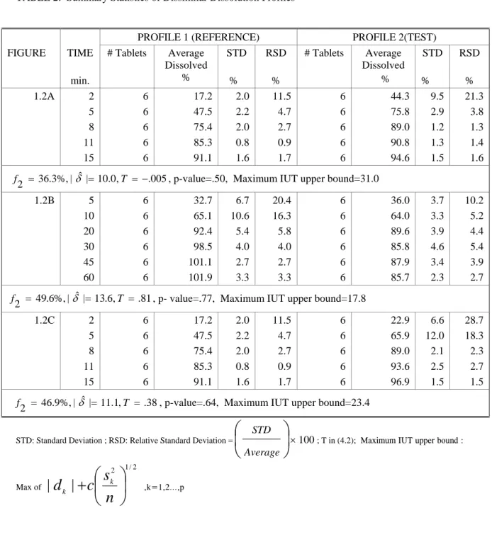
TABLE 1

SUMMARY STATISTICS OF SIMILAR DISSOLUTION PROFILES

PROFILE 1 (REFERENCE) PROFILE 2 (TEST) FIGURE TIME min. # Tablets Average Dissolved % STD % RSD % # Tablets Average Dissolved % STD % RSD % 1.1A 2 6 22.9 6.6 28.7 6 44.3 9.5 21.3 5 6 65.9 12.0 18.3 6 75.8 2.9 3.8 8 6 89.0 2.1 2.3 6 89.0 1.2 1.3 11 6 93.6 2.5 2.7 6 90.8 1.3 1.4 15 6 96.9 1.5 1.5 6 94.6 1.5 1.6 48.5%,| ˆ| 1.2, 5.3, p-value=.0009, Maximum IUT upper bound=26.0

2 = = T = − f δ 1.1B 2 6 18.1 1.4 7.8 6 21.8 1.8 8.3 5 6 65.4 7.0 10.7 6 77.8 1.9 2.4 8 6 85.4 2.0 2.3 6 89.2 1.5 1.7 10 6 87.8 2.1 2.4 6 92.7 1.5 1.6 12 6 93.7 5.6 6.0 6 94.8 1.8 1.9 20 6 97.6 4.7 4.8 6 98.8 2.3 2.3 60 6 106.3 3.2 3.1 6 107.0 1.4 1.3 f₂ =62.7%,|δˆ|= 3.6,T = −14.8, p-value <.0001, Maximum IUT upper bound=15.3

1.1C 10 12 12.0 4.4 37.0 6 13.9 8.4 60.3 20 12 28.0 6.4 22.8 6 29.1 4.0 13.9 30 12 45.9 8.8 19.2 6 48.2 5.8 12.0 45 12 61.5 10.8 17.6 6 74.0 7.7 10.5 60 12 79.6 9.0 11.3 6 90.1 1.1 1.2 56.3%,| ˆ| 0.24, 2.4, P value=.0183, Maximum IUT upper bound=16.9

2 = = T = −

f δ

STD: Standard Deviation ; RSD: Relative Standard Deviation =

⎟

×100

⎠

⎞

⎜

⎝

⎛

Average STD

; T in (4.2); Maximum IUT upper

bound : Max of 2 / 1 2

|

|

⎟

⎠

⎞

⎜

⎝

⎛

+

n

s

c

d

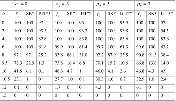
k k ,k=1,2…p

TABLE 2: Summary Statistics of Dissimilar Dissolution Profiles

PROFILE 1 (REFERENCE) PROFILE 2(TEST) FIGURE TIME min. # Tablets Average Dissolved % STD % RSD % # Tablets Average Dissolved % STD % RSD % 1.2A 2 6 17.2 2.0 11.5 6 44.3 9.5 21.3 5 6 47.5 2.2 4.7 6 75.8 2.9 3.8 8 6 75.4 2.0 2.7 6 89.0 1.2 1.3 11 6 85.3 0.8 0.9 6 90.8 1.3 1.4 15 6 91.1 1.6 1.7 6 94.6 1.5 1.6

, p-value=.50, Maximum IUT upper bound=31.0

005 . , 0 . 10 | ˆ | %, 3 . 36 2 = = T = − f δ 1.2B 5 6 32.7 6.7 20.4 6 36.0 3.7 10.2 10 6 65.1 10.6 16.3 6 64.0 3.3 5.2 20 6 92.4 5.4 5.8 6 89.6 3.9 4.4 30 6 98.5 4.0 4.0 6 85.8 4.6 5.4 45 6 101.1 2.7 2.7 6 87.9 3.4 3.9 60 6 101.9 3.3 3.3 6 85.7 2.3 2.7 81 . , 6 . 13 | ˆ | %, 6 . 49 2 = = T =

f δ , p- value=.77, Maximum IUT upper bound=17.8

1.2C 2 6 17.2 2.0 11.5 6 22.9 6.6 28.7 5 6 47.5 2.2 4.7 6 65.9 12.0 18.3 8 6 75.4 2.0 2.7 6 89.0 2.1 2.3 11 6 85.3 0.8 0.9 6 93.6 2.5 2.7 15 6 91.1 1.6 1.7 6 96.9 1.5 1.5 46.9%,| ˆ| 11.1, .38, p-value=.64, Maximum IUT upper bound=23.4

2 = = T =

f δ

STD: Standard Deviation ; RSD: Relative Standard Deviation =

⎟

×100

⎠

⎞

⎜

⎝

⎛

Average STD

; T in (4.2); Maximum IUT upper bound :

Max of 2 / 1 2

|

|

⎟

⎠

⎞

⎜

⎝

⎛

+

n

s

c

d

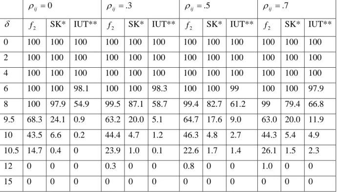
k k ,k=1,2…,p

Table 3: Percent of Experiments Accepting the Equivalency of Two Dissolution Profiles For Case 1 (early time point %RSD >20)

0

= ij

ρ ρ_ij =.3 ρ_ij =.5 ρ_ij =.7

δ f₂ SK* IUT** f₂ SK* IUT** f₂ SK* IUT** f₂ SK* IUT**

0 100 100 97 100 100 96.1 100 100 95.9 100 100 97 2 100 100 93.3 100 100 93.3 100 100 93.8 100 100 94.5 4 100 100 82.8 100 100 83.8 100 100 83.6 100 100 83.6 6 100 100 61.8 99.9 100 61.4 99.7 100 61.3 99.6 100 63.2 8 97.1 97 25.2 93.6 88.1 31.0 92.2 87.9 33.5 90.8 91.3 38.4 9.5 78.3 22.9 1.3 73.8 16.4 6.8 70.1 15.2 10.6 66.8 13.8 14.0 10 41.5 6.1 0.1 48.8 4.7 1 46.0 4.1 2.6 46.8 4.3 4.9 10.5 23.1 1 0 27.7 1.0 0.1 30.3 1.0 0.7 32.9 1.0 2.4 12 0.1 0 0 1.7 0 0 4.3 0 0 6.1 0 0 15 0 0 0 0 0 0 0 0 0 0 0 0

* Saranadasa and Krishnamoorthy; ** Intersection Union Test

Table 4: Percent of Experiments Accepting the Equivalency of Two Dissolution Profiles For Case 2 (early time point %RSD <10)

0

= ij

ρ ρij =.3 ρij =.5 ρij =.7

δ f₂ SK* IUT** f₂ SK* IUT** f₂ SK* IUT** f₂ SK* IUT**

0 100 100 100 100 100 100 100 100 100 100 100 100 2 100 100 100 100 100 100 100 100 100 100 100 100 4 100 100 100 100 100 100 100 100 100 100 100 100 6 100 100 98.1 100 100 98.3 100 100 99 100 100 97.9 8 100 97.9 54.9 99.5 87.1 58.7 99.4 82.7 61.2 99 79.4 66.8 9.5 68.3 24.1 0.9 63.2 20.0 5.1 64.7 17.6 9.0 63.0 20.0 11.9 10 43.5 6.6 0.2 44.4 4.7 1.2 46.3 4.8 2.7 44.3 5.4 4.9 10.5 14.7 0.4 0 23.9 1.0 0.1 22.6 1.7 1.4 26.1 1.5 2.3 12 0 0 0 0.3 0 0 0.8 0 0 1.0 0 0 15 0 0 0 0 0 0 0 0 0 0 0 0

* Saranadasa and Krishnamoorthy; ** Intersection Union Test