Efficiency in housing markets: Which home buyers know how to discount?
Erik Hjalmarsson
a,*, Randi Hjalmarsson
ba
Division of International Finance, Board of Governors of the Federal Reserve System, 20th and C Streets, Washington, DC 20551, USA b
School of Public Policy, University of Maryland, Van Munching Hall, College Park, Maryland 20742, USA
a r t i c l e
i n f o
Article history:
Received 30 September 2008 Accepted 19 May 2009 Available online 22 May 2009
JEL classification: G14 R21 R31 Keywords: Housing markets Market efficiency Cooperative housing
a b s t r a c t
We test for efficiency in the Swedish co-op market by examining the negative relationship between the sales price and the present value of future monthly payments or ‘rents’. If the co-op housing market is efficient, the present value of co-op rental payments due to underlying debt obligations of the coopera-tive should be fully reflected in the sales price. However, a one hundred kronor increase in the present value of future rents only leads to an approximately 75 kronor reduction in the sales price. These ineffi-ciencies are larger at the lower end of the housing market and in poorer, less educated regions and appear to reflect both liquidity constraints and the existence of more ‘sophisticated’ buyers in higher educated areas. Overall, our findings suggest that there is some systematic failure to properly discount the future stream of rent payments relative to the up front sales price.
Published by Elsevier B.V.
1. Introduction
For the majority of households, the purchase of a home is the largest financial decision of their lives. One may therefore assume that housing market transactions are conducted by agents who have carefully evaluated all available information and that the resulting prices reflect that information. A growing number of studies, many of which are based on time-series of home sales and rental data, therefore test whether housing prices are in fact informationally efficient.1This paper takes advantage of the nature of the cooperative housing market in Sweden to provide an alterna-tive test of market efficiency.
Cooperatives are distinct from condominiums in that the pur-chaser of a unit in a cooperative housing association is formally buying a share in the cooperative, along with the non-time-re-stricted right to occupy the unit, i.e. the actual apartment. Owners of a co-op unit must make a monthly payment comprised of main-tenance fees and the capital costs attributed to the cooperative’s debt. For the remainder of the paper, we will refer to the total of these monthly payments as ‘rents’. The capital costs component
derives from the fact that the formal owner of a co-op unit is the cooperative association; the cooperative can have its own debts, which are serviced through the collection of rents from the mem-bers of the cooperative, i.e. the indirect owners of the cooperative apartments. These implicit interest payments in the monthly co-op rents are on top of any direct mortgage service obligations that the home buyer may have incurred. Thus, only part of the true cost of owning a co-op unit is reflected in the actual sales price; the remaining cost is reflected in the monthly rent. The total value of a co-op unit can therefore be expressed as the sum of its sales price and the discounted value of the cooperative financing component of the future monthly rent payments, i.e. rent excluding the main-tenance fee component.
This simple present value relationship provides the starting point for our analysis. In particular, if markets are efficient, there should be an inverse one-to-one relationship between prices and discounted rents. That is, if the present value of rents goes up by one unit, prices should decrease by one unit.
Although this analysis relies on Swedish data, there is no reason to believe that the findings cannot be extended to housing markets in other countries or, indeed, to non-cooperative forms of housing. Co-ops are also quite common in many other countries, including Finland and Canada, and in certain cities in the US, such as New York, where they tend to dominate the market for owner occupied apartments.2More generally, our test of market efficiency is a test of
0378-4266/$ - see front matter Published by Elsevier B.V. doi:10.1016/j.jbankfin.2009.05.014
*Corresponding author. Tel.: +1 202 452 2426; fax: +1 202 263 4850.
E-mail addresses:erik.hjalmarsson@frb.gov(E. Hjalmarsson),rhjalmar@umd.edu (R. Hjalmarsson).
1
Most related to the current paper areMeese and Wallace (1994) and Gallin (2005). Other studies that consider aspects of housing market efficiency include (Case and Shiller, 1989, 1990; Case and Quigley, 1991; Guntermann and Norrbin, 1991; Gatzlaff, 1994; Berg and Lyhagen, 1998; Englund et al., 1999; Hill et al., 1999; Malpezzi, 1999; Rosenthal, 1999; Hwang and Quigley, 2002, 2004; Hwang et al., 2006).
2
Co-ops have also been increasing in popularity in the 1990s and 2000s in a number of U.S. cities, including Chicago, Washington, D.C, and Miami. For an extensive analysis of co-ops in New York, seeSchill et al. (2004).
Contents lists available atScienceDirect
Journal of Banking & Finance
j o u r n a l h o m e p a g e : w w w . e l s e v i e r . c o m / l o c a t e / j b fproper discounting, or comparison, of future payments relative to upfront costs. This is strongly related to traditional tests of housing market efficiency, which compare house price indices to present val-ues of rent-cost indices (e.g.,Meese and Wallace, 1994). The major drawback of this traditional approach is that rent and price indices are, for obvious reasons, not based on the same housing units or, more importantly, units that necessarily have comparable character-istics;Glaeser and Gyourko (2007)provide evidence that this is in fact the case and argue against the robustness of empirical analyses based on rent-price comparisons. In addition, these types of analyses rely on the time-series properties of the housing market data, which may be partly determined by frictions in the market;Meese and Wallace (1994)try to get around this second issue by considering tests of efficiency in the long-run, where short-run market frictions should play no role.
In contrast, by utilizing the fact that a co-op has both a price and a rent component, we can test a present value relationship by com-paring across co-op units, rather than between rental and owner occupied units. This offers several advantages. The buy versus rent decision is a very large one for most households, and may depend on many factors, not all of which are of a financial nature. By focus-ing on actual co-op purchases, we eliminate this part of the deci-sion making process and therefore expect a cleaner present value relationship. Cross-sectional transaction data also alleviates con-cerns about the time-series properties of the data. Finally, in our setup, there is a clear theoretical cross-sectional relationship be-tween rents and prices; deviations from this relationship are easily translated into actual measures of miss-pricing.3
Our analysis is based on a data set of more than 30,000 Swedish co-op transactions between 2002 and 2005 and hedonic price regressions that relate co-op sales prices to the present value of fu-ture rents.4 Our preferred specification controls for a variety of apartment characteristics, unobservable neighborhood characteris-tics through zip code fixed effects, and national and regional time trends. We find that an increase in discounted rents of 100 Swedish kronor (SEK) only leads to a decrease in price of about 75 SEK (8 SEK1 US$). On average, co-ops with high rents are thus relatively over-priced. This result cannot be explained away by potential changes in future rents or interest rates. For instance, buyers need to have extremely risk-averse beliefs regarding the paths of future interest rates to reconcile our estimates with market efficiency.
An alternative hypothesis that may explain these findings is that not all buyers have a common discount rate, as our baseline specification assumes. Rather, some may have substantially higher discount rates due to liquidity constraints; that is, home buyers who cannot make the necessary down payment will face a higher marginal mortgage rate. To explore this scenario, we redo our anal-ysis for sub-samples of the data grouped on apartment size. One may expect apartment size to be a reasonable proxy for liquidity, as poorer and first time buyers, i.e. those most likely to be con-strained, are those most likely to buy the smallest apartments. Even for the largest apartments, however, we find evidence of inef-ficiency; it is thus hard to argue that liquidity constraints can be the sole explanation for our findings. In addition, even if we allow a 2% top loan markup, which should be at the high end of the spec-trum, there is still strong evidence of inefficiency at the lower end of the market (i.e. small apartments). Thus, liquidity constraints
potentially play a role in the price formation in certain parts of the market, but cannot explain the overall inefficiency observed.
Similarly, we estimate our basic model separately for each par-ish or county in our data. We find evidence of inefficiency in 57 of 70 parishes, including those at both ends of the socioeconomic spectrum. However, these inefficiencies tend to be greater in poorer and less educated parishes. While these findings are likely to partly reflect the liquidity constraints described above, they are also consistent with there being more informed and ‘sophisti-cated’ buyers in higher educated areas who push prices closer to efficiency. Further analyses that group the data jointly on apart-ment size and education level provide evidence that both liquidity constraints and ‘sophistication’ are relevant to explain our findings. Overall, our findings suggest that there is some systematic fail-ure to properly discount the futfail-ure stream of rent payments rela-tive to the upfront sales price. This is in line with the time-series results reported in the literature, which typically show that house prices tend not to be efficient (e.gCase and Shiller, 1989, 1990; Røed Larsen and Weum, 2008). The heterogeneity across different groups of buyers is also consistent with recent findings in the emerging household finance literature. In a series of papers, Camp-bell (2006) and Calvet et al. (2007, 2008)document that higher-educated and wealthier households are more likely to satisfy the predictions of standard financial models.
The rest of the paper proceeds as follows. Section2provides background information about the Swedish co-op housing market. Section3outlines the theoretical relationship between prices and rents and discusses the calculation of the present value of future rent payments. In addition, it presents the econometric model and discusses the potential identification issue of omitted vari-ables. Section4describes the data and Section5presents the main empirical results, including an analysis of how sensitive the find-ings are to assumptions about future rents and interest rates. Sec-tion 6 explores whether the findings of inefficiency are heterogeneous across parishes and socioeconomic characteristics and discusses alternative explanations of these findings, including the potential role of risk premia. Section7concludes.
2. The Swedish cooperative market
2.1. Overview and market characteristics
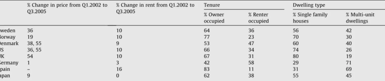
Table 1provides national housing market statistics for Sweden and a selection of other countries. During our sample period (from Q1 of 2002 to Q3 of 2005), the prices of homes and the cost of rent-ing in Sweden increased by 36 and 10%, respectively.5In 2003, 64% of Swedish homes were owner-occupied and 56% were single unit dwellings. In terms of these characteristics, Sweden is quite compa-rable to a number of other countries over the sample period, includ-ing Denmark, the US and, the UK. The change in the Swedish housinclud-ing price index shown inTable 1is also very similar to the average price change observed for our sample of co-op transactions (seeFig. 1in Section4).
Cooperative (co-op) ownership is the only way to own an apart-ment in Sweden; condominiums do not exist as an alternative. Apart from single-family houses, co-ops are therefore the only other form of owner-occupied housing, and in central areas of most cities, the only alternative to rental apartments. According to Sta-tistics Sweden, 16% of the population lived in co-ops and about 36% in rental units, as of 2001. The Swedish housing market, and especially the co-op market, is generally characterized by few mar-ket frictions and low transaction costs, including minimal mort-gage fees.
3
Røed Larsen and Weum (2008)also use price data on cooperative housing in Oslo to test for efficiency in the Norwegian housing market. In contrast to the current study, however, they focus on the time-series properties of the data and do not analyze the cross-sectional present value relationship between rents and prices, which is the focus here.
4
Linneman (1986)also relies on hedonic price regressions to determine what the ‘fair’ value of houses are and classifies the market as inefficient if the pricing errors based on the fitted hedonic regression exceed the transaction costs in the market for a substantial number of observations.
5
Note that the rent-cost indices inTable 1refer to rents on actual rental units and not the ‘rent’ on co-ops that we refer to everywhere else in the paper.
The purchase of a co-op unit entails ownership of a share of the cooperative, as well as membership in the cooperative association. The share ownership is not time-restricted in any sense. Though co-op purchasers do not have actual property rights over the apart-ment unit, they are free to renovate and otherwise modify their apartments in the same manner as a condominium owner.
Technically, a new owner of a co-op share needs to be ap-proved by the co-op board, but this is primarily a formality and rejections are extremely rare. Co-ops in Sweden are intended to be occupied by their actual owners and cannot be rented out to a third party without board approval; the co-op board does com-monly exercise its powers in this respect. There are some time limited exceptions, such as studying or working abroad for a fixed period of time, but it is usually difficult to get permission for more than a few years. The motivation behind these rules is that
the co-op is not intended as an investment vehicle but as an own-er-occupied form of living.6
The cooperative as a whole pays taxes on any potential profits as if it was a corporation, although in practice these profits are gen-erally small since there are typically no reasons or incentives to generate a profit. In addition, the cooperative also pays a property tax, equal to 0.5% of the tax value of the property, where the tax value is set to 75% of the market value of the property, calculated
as if it was a rental building. That is, the tax value of the cooperative isindependentof the market prices of the actual co-op units and also of the capital structure of the cooperative. Neither of these taxes should have any impact on the co-op buyer’s decision when choosing between a high rent and a low rent co-op unit.
As for the individual co-op owner, there existed during the sam-ple period an individual net worth tax that amounted to an annual tax of 1.5% of the total personal wealth in excess of 1.5 million SEK.7 The tax value of a co-op unit from the perspective of the net worth tax is calculated as the co-op’s share of the total tax va-lue of the cooperative minus the co-op’s share of the outstanding loans of the cooperative. Thus, to the extent that a co-op buyer has enough wealth to have to pay a net worth tax, there is a tax incentive to buy a co-op with large loans and a high rent because the calculated tax value will be lower. This consideration only ap-plies to those that are wealthy enough to be eligible to pay a net worth tax, i.e. those with a total wealth above 1.5 million, and should therefore apply primarily to those buying the largest and most expensive co-ops. If this consideration was a driving factor behind our results, we would therefore expect to see more signs of apparent inefficiency for larger co-ops, but as shown in the empirical results we find the opposite (see Section5.4). In addition, during the sample period only about 3–5% of individuals actually paid a net worth tax, further suggesting that this tax should have Table 1
Swedish and international housing market statistics. % Change in price from Q1.2002 to Q3.2005
% Change in rent from Q1.2002 to Q3.2005
Tenure Dwelling type
% Owner occupied % Renter occupied % Single family houses % Multi-unit dwellings Sweden 36 10 64 36 56 42 Norway 19 10 77 23 70 30 Denmark 38, 55 9 53 47 60 40 US 36, 55 10 66 34 74 26 UK 54 10 67 31 80 19 Germany 1 3 42 58 29 71 Spain – 16 83 11 31 69 Japan 9 0 62 38 55 45
Note: The first two columns present the total percent changes in nation-wide house-price and rent-cost indices, respectively; the rent variable here refers to rents on actual rental units and not to the monthly ‘rent’ payments for co-ops that are referred to everywhere else in the paper. The remaining four columns show the breakdown between owner-occupied and renter-occupied housing, as well as between single-family houses and multi-unit dwellings. Rent measures are based on a component of the consumer price indices. Unless otherwise stated, housing price indices are based on both new and existing dwellings.
Swedish price, rent, tenure and dwelling type data are from Statistiska centralbyrån. Tenure and dwelling type data are from 2003. Norwegian price, rent, tenure and dwelling type data are from Statistics Sentralbyra. Only price data for new, detached houses are available. Tenure and dwelling type data are from the 2001 Census. Danish price and rent data are from Danmarks Statistic. Price changes for single-family houses and owner occupied flats, respectively, are presented. Tenure and dwelling type data are for 2004. US price data are from the Office of Federal Housing Enterprise Oversight and the S&P/Case-Shiller national housing price indices, respectively. US rent data is from the Bureau of Labor Statistics. US tenure and dwelling type data are from the 2000 Census. Single family houses include mobile homes. UK rent data are from the Office for National Statistics and UK price data are from the Department of Communities and Local Government. Tenure and dwelling type data are also from the Office for National Statistics and are for 2000/2001. Single Family Houses includes detached, semi-detached, and terraced homes while multi-unit dwellings includes flats and maisonettes. Note that UK tenure and dwelling type data both include ‘other’ categories. Germany rent and price data are from Statistisches Bundesamt. The German house price index is only for existing homes. Housing tenure and dwelling type data are for 2006 and from Statistisches Bundesamt. Spanish rent data are from Instituto Nacional de Estadistica. Price data are only available starting from Q1 of 2004 from Ministerio de Vivienda and are therefore not presented. Tenure and dwelling type data are for 2001 and from Instituto Nacional de Estadistica; these also include ‘other’ categories. Japanese rent data are from the Ministry of Internal Affairs and Communications and price data are from the Japan Real Estate Research Institute. The Japanese price index is based on the Tokyo metropolitan area condo market.
0 250000 500000 750000 1000000 1250000 1500000
Average Transaction Price (kronor)
0 5 10 15
Quarter (1 = Q1 of 2002)
Fig. 1.Average quarterly co-op transaction price from 2002 to 2005.
6
Turner (1997)provides some additional information on the cooperative housing market in Sweden.
7
That is, the net worth tax is a tax on the value of the actual capital ‘stock’ of an individual, and not on the capital gains. This tax was abolished in 2007.
a very limited effect.8It is therefore highly unlikely that tax consid-erations are the driving factor behind our findings of market inefficiency.
2.2. Rent determination
The cooperative association faces two sorts of costs. First, there are the costs of maintaining all interior and exterior common areas as well as other maintenance costs that may be shared among the members. Second, the cooperative as a whole may have loans that need to be serviced. These costs are met by collecting monthly pay-ments, or ‘rents’, from the association members, which are based on the size of their shares in the cooperative and typically are fairly linear functions of apartment size.
When a co-op is initially formed and the shares are sold, either by a residential developer or through a conversion of rental units to co-op units, the founders can decide how much of the total cost of the shares will be paid upfront by the buyers and how much of it will be financed by mortgages taken out by the cooperative itself. If the cooperative opts to finance a larger amount, then higher monthly rents are necessary. Ceteris paribus, higher rents should therefore imply a lower price. It should be stressed that given the size of an apartment’s share in the cooperative, the rent will not be affected by individual characteristics of the apartment. That is, if an apartment gets renovated by the current owner, the in-creased standard of the apartment will only be reflected in the price of the apartment when it is next sold, not in its rent.
Differences in the capital cost component of the rent can thus arise from differences in the initial loans taken out by the cooper-ative at the time of its foundation.9In addition, a cooperative may at times acquire new loans to finance major renovations that are con-ducted by the cooperative as a whole, such as changing the electric-ity or sewage systems in the entire building. The initial variation is clearly predetermined and exogenous to our analysis. However, if the buyer of a certain co-op expects future renovations and, conse-quently, rent increases to occur, this could bias our results since the buyer perceives the long-run rent as higher than what we ob-serve. Of course, this is only a problem for anticipated renovations, and subsequent rent increases.10Our empirical analysis therefore in-cludes a test of whether such rent increases are in fact anticipated and finds no evidence that they are.
3. Modeling the relationship between prices and rents
The purpose of this paper is to estimate the degree to which dif-fering rents across apartments are accounted for in the sales prices of co-ops. The basic idea is that given two identical apartments with different rents, the difference in price between the two apart-ments should equal the difference between the present values of all future rent payments. To account for the fact that apartments differ in dimensions other than rents, we rely on hedonic price regressions and control for a variety of apartment and neighbor-hood characteristics as well as trends over time.
3.1. Theoretical motivation
As discussed previously, the rent on a co-op is comprised of a maintenance fee component and a capital cost component, which covers the cooperatives’ financial costs in terms of mortgages and loans. In effect, a co-op purchaser takes on a share of the coop-eratives’ debt obligations, commensurate with the size of his share in the cooperative. Thus, the true price, or intrinsic value, of the co-op is actually the sum of the sales price and the present value of this future stream of capital cost payments. Consequently, the sales price should equal the intrinsic value less the present value of the capital cost payments. That is, for co-opi,
Pi¼ViPVðCiÞ; ð1Þ
wherePiis the sales price,Viis the intrinsic value, andCiis the cap-ital cost component of the rent.
Eq.(1)captures the fundamental relationship that should hold between prices and discounted rents, if co-ops are priced effi-ciently. The primary aim of this paper is to evaluate the empirical validity of this theoretical relationship and test whether the pres-ent value of the future rpres-ent paympres-ents, PV(Ci), is in fact fully re-flected in the sales price,Pi. Thus, if the variables in Eq.(1)were all observed, one could run the empirical regression,
PiVi¼hPVðCiÞ þ
g
i; ð2Þwhere it follows that under rational, or efficient, pricing, h=1. However, since the intrinsic valueViis not observed, Eq.(2)is not a directly testable relationship.
We therefore rely on hedonic price regressions to test this rela-tionship. In such a framework, it is assumed that a vector of char-acteristics capture the value of the good. That is,
Vi¼Xibþ
1
i; ð3ÞwhereXiincludes the relevant characteristics of the co-op and
1
iis a mean zero error term uncorrelated withXi. Consequently,Pi¼hPVðCiÞ þXibþ
e
i; ð4Þwhere, under the null hypothesis of efficient pricing,h=1.
3.2. Calculating the present value of the rent
Consider two co-ops that have the same intrinsic value, but one costsP1and the otherP2, and assume that the home buyers borrow at the prevailing mortgage ratem. If the efficient market hypothe-sis holds, it follows that the annual capital costs for these two co-ops should be identical:
ð1
s
ÞmP1þC1¼ ð1s
ÞmP2þC2; ð5Þ wheres
is the tax rate at which interest rate payments are deduct-ible andC1 andC2are the annual capital cost components of the rents.11,12 Divide through by the effective interest rate, (1s
)m, and it follows that8
These figures are based on information obtained from the Swedish tax authority, which shows that for 2002-2005 between 230 to 330 thousand individuals paid net worth taxes each year, out of a total population of about seven million people that are above 18 years old.
9
It is not clear what determines the proportions in this initial split. Indeed, given that the cooperative generally enjoys less advantageous tax deductions on its loans, it would typically be more efficient for the individual buyers to pay the total value of the co-op unit directly and carry all of the capital costs in the form of private mortgages.
10 Cooperatives typically have funds put aside over time to at least partially cover
the costs of future renovations. Thus, many anticipated renovations should cause only minor, and most likely transient, changes in rents.
11
The mortgage ratemis the rate faced by the individual purchaser of the co-op. While the rate faced by the cooperatives may differ fromm(and across cooperatives), this is reflected in the capital costs,C1andC2, which represent the servicing costs of
their mortgages at the cooperatives’ prevailing mortgage rates. SinceC1andC2are
taken as given in our analysis, the cooperatives’ mortgage rates do not explicitly enter into our analysis. To the extent that the cooperatives’ interest rate payments are tax deductible, this will also already be reflected in the values of C1and C2, which
explains why the personal mortgage payments are tax adjusted, but notC1andC2; no
portion of the rent (i.e. the capital cost or maintenance fee) is tax deductible by the individual co-op purchaser.
12
In practice, the home buyer might not borrow the entire amount, and the prevailing mortgage rate might therefore not represent, on average, the true cost of capital for the home buyer. However, it is reasonable to assume that at the margin, most home buyers will borrow at the prevailing mortgage rate. In particular, it seems a natural assumption that the marginal cost of capital is equal to the mortgage rate when choosing between two co-ops with different sales prices.
P1þ
C1
ð1
s
Þm¼P2þC2
ð1
s
Þm: ð6ÞThe terms on each side of this equation are, of course, equal to the price plus the discounted value of the future rent payments, under the assumption of a fixed discount rate equal to the (tax-adjusted) mortgage rate, (1
s
)m, and fixed rents. The present value of the rent can easily be adjusted to allow for changing rents. Suppose rents were to decrease byapercent every year after the first year. In this case, it follows thatPVðfCðtÞg1t¼1Þ ¼ X1 t¼1 CðtÞ ð1þ ð1
s
ÞmÞt¼ X1 t¼1 ð1aÞt1Cð1Þ ð1þ ð1s
ÞmÞt ¼ Cð1Þ ð1s
Þmþa: ð7ÞThe capital cost part of the rent reflects the servicing of loans that the cooperative as a whole has incurred. If the rent covers only the interest rate payments on these loans, one would expect the rent to stay fixed in the future since the loan remains the same each year, provided interest rates stay constant. On the other hand, if the rent payments also include an amortization on these loans, one would expect the rent to decrease over time as the loan becomes smaller. That is, if the cooperative were to pay off 1% of their loans each year, this should translate into an average decrease in the rent of 1% per year. In practice, there might be a desire to smooth rents and decreases in the loan might therefore not be immediately re-flected in the rents, but over the long-run, the relationship should hold. We discuss plausible levels of rent decreases and amortization rates in the empirical section.13Use of Eq.(7)to calculate present values also assumes that the rent payments continue indefinitely in the future. We find no evidence to the contrary when looking at annual statements for more than 100 cooperatives in Gothenburg; thus, most loans that cooperatives have are, for our purposes, infi-nitely lived. That is, the rents paid to service these loans cover only interest rate payments plus the potential (proportional) amortiza-tion rates discussed in the empirical secamortiza-tion.14
We thus calculate the present value of future discounted rents asCi/ki, whereki= ((1
s
)mi+ai) andmiis the mortgage rate faced by the purchaser of co-opi,aiis the rent decrease or, alternatively interpreted, the amortization rate, ands
is the tax rate at which interest rate payments are deductible and equal to 30%; the 30% tax deduction applies to all home owners in Sweden, regardless of their income level. In addition, the effect of changing future interest rates is explicitly addressed in the empirical sections.The discount factor proposed here is somewhat different from the one used, for instance, by, Meese and Wallace (1994). It is worth briefly discussing the differences, which stem from the fact that we compare co-op units with each other rather than rental apartments with owner occupied residences, as done by Meese and Wallace. Similar to Meese and Wallace, we use the mortgage rate adjusted for (income) tax deductions as the basic interest rate component in the discount rate. However, Meese and Wallace also adjust for property taxes, depreciation, and rental inflation. In our setup, property taxes are paid for by the cooperative as a whole and are not linked to the purchase prices of the individual units; rather, they are determined by the value of the entire cooperative and are thus independent of the capital structure. The depreciation term in Meese and Wallace accounts for the capital depreciation of the home-owner’s property, which is a cost that is not incurred
when renting. However, in the context of our application, capital depreciation does not affect the trade off between purchase prices and rents since it should be the same across units, once other fac-tors have been controlled for. Similarly, rental inflation plays no role in our analysis. Finally, Meese and Wallace also include a risk premium on housing investments. While this could also be added to our current discount factor, its interpretation is not as straight-forward since we are comparing between investments in co-ops rather than between buying and renting. However, since the per-sonal mortgage is in a sense riskier to the home buyer than the mortgage carried by the cooperative, which has a form of limited liability attached to it from the perspective of the individual home buyer, a risk premium could be added to the discount factor. Be-cause there is no obvious way of estimating this premium, we as-sume throughout the analysis that it is zero, but discuss it qualitatively at the end of Section6.
3.3. Total rent, capital costs, and maintenance fees
An additional empirical issue that must be dealt with is the fact that the capital cost component of the rent is not directly observed in our data; rather, we only observe the total rent, i.e. maintenance plus capital costs. Therefore, we rewrite Eq.(4), letting the total an-nual rent of co-opiberenti=Ci+Mi, whereCiandMidenote the an-nual capital cost and maintenance components of the rent, respectively: Pi¼hPVðCiÞ þXibþ
e
i¼h Ci ki þhMi ki hMi ki þXibþe
i ¼hrenti ki hMi ki þ Xibþe
i: ð8ÞThus, the coefficient in front of the total rent is still identical to the original one in front of the capital cost component, but an additional variable,Mi/ki, which represents the discounted value of the main-tenance fee, is now present. To control for this additional term empirically, we proxy for the maintenance fee with a linear combi-nation of the characteristics inXi. That is, under the assumption that
Mi=Xik, it follows that Pi¼h renti ki Xi ki khþXibþ
e
ih renti ki þXi kiu
þXibþe
i: ð9ÞThis effectively assumes that conditional onXi, the maintenance fee is constant. For instance, ifXirepresents the size of the co-op, the maintenance fee per square meter would be equal across coopera-tives. More generally, potential differences in the maintenance fee across other apartment or neighborhood characteristics can also be controlled for by interacting these observable control variables (or neighborhood dummies) with the inverse of the discount rate. Empirically, however, it is evident that once we interact the square meter size of the co-op with the inverse of the discount rate, addi-tional interaction terms (such as floor, number of floors, and parish dummies) do not alter the results. There is thus strong support for the notion that the maintenance fee per square meter is fairly con-stant across cooperatives in the sample. This is consistent with the nature of typical Swedish housing cooperatives, i.e. they generally have no common area rooms or other elements, such as pools or doormen, that would add variation to the maintenance fee.
3.4. Empirical specification
The basic specification taken to the data is presented in Eq.(10). The dependent variable,P, is the sales price for transactionion day
t, and in parishyand zip codez.
Pityz¼
a
þh rentityz ki þXityz kiu
þAityzbþQtc
þParishyd þ ðParish yTtÞkþZipz/þe
ityz: ð10Þ13 As discussed previously, new loans could also be taken on due to the need, for
instance, to raise new capital for major renovations. This could raise rents in the future and we explicitly address this possibility in the empirical section.
14
That is, we do not find evidence of cooperatives paying off their loans with fixed monthly payments rather than in proportional amounts, which supports our hypothesis that the rate of amortization translates into an equivalent rent decrease and that the loans are, for our purposes, infinitely lived.
Thus, the aim of this paper is to test whetherhis significantly dif-ferent from negative one. We control for a number of observable and unobservable characteristics. Specifically,Aincludes apartment characteristics, such as size, number of rooms, floor number, num-ber of floors in the building, building age, and whether or not heat is included in the rent. We use quarterly dummies (Q) to control for the increasing trend in co-op prices observed nationwide over the sample period. In addition, we allow for the possibility that trends vary across geographic areas by including parish specific time trends (ParishyTt). In Sweden, a parish is comparable to a US county. Of course, given the cross-sectional nature of our analysis, one must also address the concern of omitted variable bias. In particu-lar, an omitted variable that is positively correlated with both price and rents would bias our results away from market efficiency and towards a coefficient of zero.15The most obvious omission is a mea-sure of the overall standard of the apartment. Unfortunately, the available data does not include any variables, such as whether the kitchen has been renovated, that would help characterize apartment quality. We do not believe that this is as problematic as it may seem for two reasons. First, strict building codes in conjunction with thin tails in the income distribution contribute to fairly homogeneous housing standards in Sweden. Second, many indicators of standard are unlikely to be correlated with the rent; specifically, idiosyncratic upgrades done by the co-op owner, such as a kitchen renovation, would be reflected in the price of an apartment but not in the rent, as discussed previously.
Of course, not all variation in standard is idiosyncratic across units. It is certainly feasible that some cooperatives with an overall greater standard have a higher level of debt. Such overall building standard may be neighborhood specific; for instance, cooperatives in wealthy neighborhoods may be more inclined to invest money in the building to keep it in superior condition, thereby keeping rents high. To the extent that this is the case, we control for unob-servable neighborhood characteristics in two ways. First, we con-trol for parish dummies,Parishy. However, it is certainly possible that neighborhood characteristics vary within a parish. Thus, our preferred specifications also include neighborhood fixed effects in the form of zip code dummies, Zipz. There are 77 parishes and 1081 zip codes in our data.16
There is, of course, the possibility that the neighborhood fixed effects do not control for all unobservables. For instance, to the ex-tent that there is variation in apartment standard within neighbor-hoods that is correlated with monthly rents, our estimated rent coefficient may still suffer from omitted variable bias. This is a problem, however, that is common to many cross-sectional stud-ies, including hedonic price regressions. As stated above, this may be less of a concern in our Swedish data than in some other contexts.
4. Data
Our data set consists of over 30,000 transactions of Swedish co-ops between January 2002 and September 2005 for the three larg-est cities in Sweden: Stockholm, Gothenburg, and Malmo.17 The data come from a company called Värderingsdata AB, which collects data on all co-op transactions conducted by members of Svenska Mäklarsamfundet (the Swedish association of real estate agents), as well as by Föreningssparbankens Fastighetsbyrå and Svensk Fast-ighetsförmedling, which are the two largest real estate agencies on the market. The data is believed to cover approximately 70% of all co-op transactions that occur in Sweden.
For each transaction, the following data are recorded: the trans-action date, the actual sales price, the annual rent, the size of the apartment measured in square meters, the number of rooms, the apartment’s floor number, the number of floors in the building, the build year, and whether heating is included in the rent.18 In addition, the address of the apartment, including the zip code and parish, and the name of the co-op in which it is sold are reported.
Table 2presents summary statistics for the entire sample. The average price of co-ops sold is 1,250,685 SEK; at an exchange rate of 8.0 SEK per US dollar, this is approximately $156,300. Prices vary substantially across the three cities, ranging from an average of 1.6 million SEK in Stockholm to 1.0 million SEK in Gothenburg and just 0.7 million SEK in Malmo.Fig. 1plots the average transac-tion price for each quarter from January 2002 through September 2005, and indicates an increase of more than 35% over the period. The average annual rent is 37,629 SEK across all cities. Com-pared to the price, there is much less variation in the annual rent across cities and over time; the average annual rents in the first and last quarters, respectively, are 37,307 SEK and 37,232 SEK. To calculate the present value of future rent payments, we rely on the mortgage rate as of the transaction date. This is measured as the average of the five-year rates from three different lenders (SBAB, Nordea, and Stadshypotek); the average mortgage rate faced by purchasers in our sample is 4.8% and decreases substan-tially over the sample period from 6.7%, on average, in the first quarter to 3.6% in the final quarter. Assuming no amortizations, the average present value of future rent payments is 1,150,926 SEK. Thus, the present value of future rent payments is not an inconsequential amount; on average, it almost equals the purchase price.19
The average apartment in the entire sample is 66 square meters and two-room apartments are the most common. Overall, 73% of the co-ops include heat in the rent. Seven mutually exclusive vari-ables are created to indicate the age of an apartment, where the age is defined to be the transaction year minus the build year. Overall, 5.2% of the units are less than 10 years old and about two-thirds of the units are more than 50 years old.
15
However, it is also possible, though perhaps less likely, that omitted variables are not positively correlated with both rent and prices. For instance, high rents, and consequently large debt levels, might in some circumstances send a signal that the cooperative is poorly managed or in some economic distress. If high rents were indeed a signal of economic problems for the cooperatives, one would expect low rent apartments to be relatively more attractive than high rent apartments; that is, the coefficient in front of the discounted rent,h, should be less than minus one in an efficient market. Given that we consistently findhto be greater than minus one in the empirical results, we do not investigate this conjecture further. However, it potentially adds to the strength with which we reject the efficient market hypothesis.
16
Note that it is possible, though not common, for a zip code to be located in more than one parish; thus parish and zip code fixed effects can be included simultaneously in the analysis. In addition, note thatTable 2presents within parish and within zip code standard deviations for each of the variables; i.e. the standard deviation after subtracting the parish or zip code mean from each observation. While there is slightly less variation within parishes and zip codes than in the entire sample, there is still a sufficient amount of variation for identification.
17 It should be noted that this data is only representative of completed transactions,
i.e. where the seller and buyer agree on a price, and not all co-ops listed on the market.
18 In Sweden, ‘number of rooms’ refers to the number of rooms besides the kitchen
and bathroom. So, a one-room apartment is a studio, a two-room apartment is a one bedroom, etc. Number of bathrooms is not reported in the data; but, this is largely a reflection of the lack of emphasis placed on bathrooms in the market.
19
As stated previously, we do not directly have data on the size of the capital component of the rent. To give a ballpark estimate of the present value of the capital cost component by itself, one can assume a maintenance fee of 350 SEK per square meter; this appears to be a reasonable estimate based on annual statements from Swedish cooperatives. In this scenario, the average discounted value of the capital component of the rent is 448,351 SEK, which is still almost 40 percent of the average sales price. As discussed previously, however, our empirical analysis is based on the total rent and not this back-of-the-envelope calculation.
5. Empirical results
5.1. Baseline results
Table 3presents the main empirical results. The baseline spec-ifications are presented in Panel 1; the remaining panels ofTable 3 allow for rent decreases or, equivalently, amortization of the coop-eratives’ loans. The first row of columns (1) and (2) of each panel present the coefficient on the present value of the discounted rent stream that results from estimating Eq.(10)when zip code fixed effects are excluded and included, respectively. Whether or not the estimated rent coefficients differ significantly from minus one, i.e. the value under the null hypothesis of market efficiency, are indicated with stars throughout the tables.
As seen in columns (1) and (2) of Panel 1, the estimated rent coefficient is equal to0.61 when zip code fixed effects are not in-cluded and equal to0.56 with zip code fixed effects.20That is, on average, increasing the present value of the annual rent by 100 SEK decreases the transaction price by 56–61 SEK. Thus, the results so far strongly reject the efficient market hypothesis. Given the concerns about omitted variables, our preferred specification includes zip code fixed effects to control for neighborhood unobservables. Includ-ing zip code fixed effects does not decrease the precision of the esti-mates; in fact, the standard errors actually decrease somewhat (from 0.03 to 0.02).
5.2. Rent changes
We continue the analysis by assessing the sensitivity of these baseline estimates to relaxing the assumptions that future rents and mortgage rates will not change. Specifically, Panels 2 and 3 ofTable 3assume an annual rent decrease or, equivalently, amor-tization rate of 1% and 2%, respectively. Intuitively, and as is evi-dent from the discount formula presented in Eq. (7), rent decreases will result in a lower present value of future rents; there-fore,^hmust increase in absolute value. With zip code fixed effects included, assuming a 1% amortization rate results in a rent
coeffi-cient of0.74 that is highly significantly different from minus one. Increasing the amortization rate to 2% brings the rent coefficient much closer to minus one, although the point estimate of0.92 is still significantly different.
As is evident, decreasing rents or amortizations can substan-tially impact the results; it is therefore important to identify the value of a realistic amortization rate. To get a sense of this, we examined the annual statements from 125 cooperatives in Gothen-burg and recorded the amortization rate of their loans as well as the change in overall rents.21 The results are shown in Table 4. The average change in overall rent from one year to the next for the 125 cooperatives is 1.2%; this is very similar to the average an-nual increase in rent per square meter of 1.3% observed in our pri-mary data. As is seen from the percentiles of the rent changes, very few of these 125 cooperatives lower their rents, although more than half keep their rents fixed for the year of the annual statement. As discussed previously, short term rent changes may not reflect ex-pected longer term patterns that might result from persistent annual amortization of the cooperatives’ loans. The average amortization rate is 1.7%, although this may be somewhat misleading since the median rate is only 0.53%. The high average is driven by a few large amortizations, which were primarily the results of some windfall gain for the cooperative, such as the conversion and sale of previous rental apartments. These high amortization rates are therefore al-most exclusively one time events and do not represent long-term averages. The final row in the table gives the statistics for those cooperatives that amortized between 0% and 5% of their loans, and for which the average amortization rate is 0.71%.
Therefore, based on a reading of the annual statements, we be-lieve that a long-term average amortization rate closer to 1% (and probably even lower than 1%) is more realistic than a 2% rate. That is, the results in Panel 2 ofTable 3should provide the most accu-rate estimated rent coefficient (i.e.0.74).
A separate issue that is also related to rent changes is whether co-ops with relatively low rents today have some unobservable Table 2
Summary statistics.
Variable Mean Std. Dev. Within Parish Std. Dev.a
Within Zipcode Std. Dev.b
Min Max
Price (kronor) 1,250,685 934,297 706,249 614,146 17,500 9,450,000
Price per Meter2
19,903 11,436 5120 4420 179 86,667
Annual rent (kronor) 37,629 17,022 15,541 12,499 0 199,044
PV annual rent (kronor) 1,150,926 562,249 520,712 439,384 0 4,335,367
Meter2 65.78 27.19 25.39 22.09 12 276 1 Room 0.18 0.39 0.37 0.35 0 1 2 Rooms 0.42 0.49 0.48 0.46 0 1 3 Rooms 0.25 0.43 0.42 0.40 0 1 4 Rooms 0.11 0.31 0.31 0.29 0 1 5 or More rooms 0.037 0.19 0.19 0.17 0 1 Floor 2.85 1.70 1.64 1.49 1 21 # Floors 4.73 2.02 1.82 1.36 1 24 Heat 0.73 0.44 0.43 0.42 0 1 Stockholm 0.51 0.50 0.066 0 0 1 Malmo 0.22 0.42 0.049 0 0 1 Gothenburg 0.26 0.44 0.058 0 0 1 < 0 Years old 0.052 0.22 0.21 0.14 0 1 10–20 Years old 0.061 0.24 0.23 0.17 0 1 20–30 Years old 0.049 0.22 0.19 0.15 0 1 30–40 Years old 0.076 0.27 0.23 0.19 0 1 40–50 Years old 0.094 0.29 0.26 0.20 0 1 50–60 Years old 0.29 0.45 0.42 0.37 0 1 > 60 Years old 0.38 0.48 0.38 0.30 0 1 Mortgage rate 0.048 0.0086 0.0085 0.0083 0.035 0.070 a
Within standard deviation is the variation within parishes. There are 77 parishes in the sample and 30,479 observations in total.
b
Within standard deviation is the variation within zip codes. There are 1081 zip codes in the sample and 30,479 observations in total.
20
Throughout the paper, all analyses use robust standard errors that are clustered at the parish-level.
21
The annual statements were obtained from the website of the real estate agent Ahre,www.ahre.se. Most of the statements cover either the year 2004 or 2005. In cases where there were multiple years available for one cooperative, we recorded the results from the most recent statement.
characteristics that make them more likely to have higher rents in the future. For example, low rents today may signal that renova-tions have not recently taken place and are thus more likely to oc-cur in the near future. If this is true, then we are clearly underestimating the magnitude of the coefficient since low rent apartments will seem more attractive to the researcher than to the actual homebuyer, who can infer that rents are likely to in-crease in the future. Of course, whether or not this is actually an issue in our empirical analysis depends on whether homebuyers take such potential rent increases into account.
We test this by taking advantage of the fact that our data con-tains multiple transactions within the same cooperative. We iden-tify a subset of cooperatives that potentially incurred significant renovations over the sample period, as proxied for by those coop-eratives with large rent increases between the first and last
ob-served transactions. Specifically, we observe 602 cooperatives in which the annual rent per squared meter increased by more than 15%, 384 cooperatives in which it increased by at least 20%, and 253 cooperatives in which it increased by at least 25%. We then estimate Eq. (10), excluding parish specific time trends and zip code fixed effects, separately for these sub-samples of first and last transactions. The estimated rent coefficients are presented inTable 5.22
Table 3
Main results: the relationship between the present value of rents and prices.
Panel 1: Baseline specifications Panel 2: Assumes 1% amortization or rent change Panel 3: Assumes 2% amortization or rent change
(1) (2) (1) (2) (1) (2) PV annual rent 0.61*** 0.56*** 0.81*** 0.74*** 1.00 0.92*** (0.03) (0.02) (0.04) (0.03) (0.05) (0.03) Meter2 /discount rate 580.49*** 556.29*** 889.71*** 858.76*** 1251.55*** 1213.45*** (33.28) (26.90) (55.74) (47.42) (84.23) (73.77) Meter2 11255.88*** 11126.89*** 8330.42*** 8226.15*** 5474.08** 5387.27** (2545.26) (2510.50) (2538.57) (2469.69) (2571.06) (2464.50) (Meter2)2 17.46 15.38 17.63 15.44 17.79 15.55 (11.88) (11.11) (11.81) (11.04) (11.77) (11.00) 1 Room 241239.08*** 200195.51*** 241028.69*** 199926.45*** 241164.15*** 200087.21*** (79433.96) (72701.20) (79227.66) (72494.96) (79105.32) (72373.00) 2 Rooms 280674.19*** 233813.92*** 280628.11*** 233699.23*** 280859.77*** 233954.37*** (71521.99) (65055.43) (71317.57) (64820.78) (71201.06) (64687.99) 3 Rooms 255070.18*** 212065.76*** 255365.27*** 212133.58*** 255740.19*** 212432.83*** (59758.85) (53361.58) (59565.74) (53147.19) (59455.75) (53025.50) 4 Rooms 181657.75*** 158118.47*** 182283.63*** 158574.82*** 182758.57*** 158980.05*** (42588.27) (38777.54) (42505.71) (38708.78) (42469.45) (38676.41) Floor 35188.55*** 35397.63*** 35318.80*** 35524.84*** 35385.95*** 35588.90*** (4786.49) (4732.94) (4802.67) (4747.05) (4812.52) (4755.90) # Floors 11045.60** 3824.09 11109.26** 3850.35 11140.86** 3861.22 (4573.03) (2716.37) (4574.30) (2720.53) (4575.47) (2723.81) Heat 1637.66 379.29 1467.51 587.14 1391.77 688.43 (7523.14) (5821.00) (7478.91) (5832.61) (7,455.10) (5,842.48) 10–20 Years old 224,058.49*** 135430.97*** 224585.86*** 139068.26*** 225144.86*** 141618.70*** (55504.88) (48085.29) (55488.60) (47915.21) (55474.77) (47806.06) 20–30 Years old 286181.97*** 164090.86*** 291606.02*** 171036.66*** 294427.70*** 174938.11*** (64931.95) (47794.73) (64838.18) (47549.33) (64773.29) (47424.35) 30–40 Years old 309,361.45*** 183188.18*** 314507.39*** 189037.28*** 316960.22*** 192097.49*** (57,500.95) (44331.12) (57293.49) (44064.67) (57178.64) (43924.02) 40–50 Years old 241103.39*** 137920.21*** 245881.37*** 143074.28*** 248043.49*** 145638.31*** (55045.47) (43073.21) (54884.63) (42889.24) (54795.14) (42802.47) 50–60 Years old 145779.93** 99457.99** 150183.88** 104791.85** 152329.11*** 107648.87** (57186.24) (41,546.63) (56975.72) (41239.28) (56863.35) (41076.06) > 60 Years old 118056.31* 96871.18* 122585.05* 102343.08** 124758.56* 105268.86** (62979.64) (50046.04) (62843.18) (49758.88) (62777.91) (49610.18) Controls for:
Quarter dummies Yes Yes Yes Yes Yes Yes
Parish dummies Yes Yes Yes Yes Yes Yes
Parish specific time trends Yes Yes Yes Yes Yes Yes
Zip code dummies No Yes No Yes No Yes
Discount rate assumes:
30% Tax deduction Yes Yes Yes Yes Yes Yes
1% Amortization No No Yes Yes No No
2% Amortization No No No No Yes Yes
Observations 30,475 30,475 30,475 30,475 30,475 30,475
R-squared 0.85 0.89 0.85 0.89 0.85 0.89
Note: Robust standard errors that are clustered at the parish level are in parentheses. For thePV Annual Rentcoefficient, the *’s indicate a significant difference from minus one; for all other coefficients, the *’s indicate a significant difference from zero. The discount rate in Panel 1 is calculated using a 30% tax deduction. In panels 2 and 3, respectively, amortization rates of 1% and 2% are also included. Columns (1) and (2) of each panel estimate Eq.(10)when excluding and including zip code fixed effects, respectively. The omitted category for number of rooms is5 or more roomsand for apartment age is <than 10 years old.
*Indicate significance at the 10% level. **Indicate significance at the 5% level. ***Indicate significance at the 1% level.
22
While we can identify multiple transactions for the same cooperative, we cannot, unfortunately, take advantage of this in our main specifications by including cooperative fixed effects. As should be expected, there is very little variation in rent per square meter within cooperatives. That is, apart from special circumstances, there is little change in the debt structure and, hence, rents within the cooperative over our fairly short sample period.
If such renovations and subsequent rent increases are fully anticipated, then the rent coefficients for the post-renovation transactions should be less biased since the researcher and home-buyer have more similar information than in the pre-renovation transactions. Hence, the post-renovation coefficients should be clo-ser to minus one. However, the estimates shown inTable 5indicate the exact opposite. For instance, when considering the sample of cooperatives with a 15% or more rent increase, we find that the estimated rent coefficient decreases in magnitude from0.70 for the pre-renovation transactions to0.46 for the post-renovation transactions. The same pattern of results is seen for the coopera-tives with 20 and 25% rent increases, though the estimates become more imprecise due to the decreased sample sizes. Thus, there is little evidence that this kind of rent increase is anticipated and that our empirical analysis would be biased by omitting expectations about future renovations and subsequent rent changes.
5.3. Interest rate changes over time
The interest rate used in the discount formula, which is equal to the five-year mortgage rate, obviously has a large effect on the present value of the discounted rent.23The interest rate is fairly low during parts of the sample, particularly towards the end (3.6% during the last quarter); this is most likely well below what can be expected over the long-run. Thus, there might be some concern that our findings can be explained by expectations about interest rates
increasing in the future, which would reduce the present value of fu-ture rent payments.
A first diagnostic of the validity of these concerns is to see if the rent coefficient changes dramatically over the sample period. If the evidence of market inefficiency is due to a failure to account for expectations about high future interest rates, we would expect the rent coefficient to be closer to efficiency at the beginning of the sample, where the interest rate is closer to a long-run average. Although not shown here, estimating Eq.(10)quarter by quarter indicates that the rent coefficient does not change systematically over time. Thus, the results are not driven by lower discount rates at the end of the sample.
Alternatively, we can estimate the implied interest rate for each quarter that is consistent with market efficiency. That is, we set h=1, and treat the interest rate as the free parameter to be esti-mated. We still assume a 30% tax-deduction, but that there is no amortization. For each quarter,Fig. 2plots the actual five-year rate as well as two estimates of the implied interest rate. The first esti-mate shows the implied interest rate that would have to prevail in
allfuture periods in order for market efficiency to hold. The second estimate is the implied rate necessary in all periods after the first five years, assuming that the current five-year rate is used to dis-count during the initial five years. On average, the implied rate is about three percentage points higher than the five-year mortgage rate in each quarter, and ranges from about 10% in the first quarter to 6% in the last. Apart from a couple of outliers, which are most likely due to less precision in the quarterly estimates, the implied interest rate when the current five-year rate is used for the first five years is substantially higher and varies between approxi-mately 16% and 10%.
Though five-year fixed rate loans are available, many home buyers still choose floating interest rates. It is therefore reason-able to assume that most of the uncertainty (and risk-aversion) Table 4
Descriptive statistics of amortization and annual rent changes in sample of Gothenburg cooperatives.
N Mean Std. Dev. Percentile
10% 25% 50% 75% 90%
% Change in rent 125 1.24 8.76 0.00 0.00 0.00 2.00 7.00
Amortization rate (%) 125 1.70 7.82 0.00 0.00 0.53 1.67 7.27
For Cooperatives with Amortization Rates Between 0 and 5%:
Amortization Rate (%) 103 0.71 0.86 0.00 0.00 0.35 1.06 2.09
Note: Data in this table is based on annual statements for 125 cooperatives in Gothenburg. Almost all of the annual statements were from either 2004 or 2005.
Table 5
Are changes in rent expected? A within cooperative analysis.
First transaction in cooperative over the sample period Last transaction in cooperative over the sample period
Cooperatives with at least 15% increase in annual rent per meter squared between first and last transactions (N = 602)
PDV annual rent 0.70*** 0.46***
(0.09) (0.08)
Cooperatives with at least 20% increase in annual rent per meter squared between first and last transactions (N = 384)
PDV annual rent 0.82 0.45***
(0.16) (0.10)
Cooperatives with at least 25% increase in annual rent per meter squared between first and last transactions (N = 253)
PDV annual rent 0.90 0.48***
(0.25) (0.13)
Note: Robust standard errors in parentheses. We cannot directly observe which cooperatives underwent renovations. However, we proxy for this by considering those cooperatives that had a large increase in the annual rent per square meter between the first and last transactions (i.e. a 15%, 20% or 25% increase). We then use the sub-samples of first and last transactions to estimate our basic model. Specifically, each cell presents the coefficient on the present value of annual rents that result from estimating Eq.(10)when excluding parish specific time trends and zip code fixed effects. All specifications still include controls for apartment size (as a quadratic), dummy variables indicating the number of rooms, dummy variables indicating the age of the building, the floor of the apartment, the number of floors in the building, whether heat is included in the rent, and apartment size over the discount rate. The discount rate takes into account the 30% tax deduction in all specifications.
*
Indicate significantly different from minus one at 10% level.
**
Indicate significantly different from minus one at 5% level.
***Indicate significantly different from minus one at 1% level.
23
The five year fixed-rate mortgage interest rate that we use should be a conservative (high) estimate of the interest rate facing the home buyer at the time of the purchase, given that most home buyers in Sweden take at least a part of their loans with a floating rate. For instance, according to the mortgage lender SBAB’s website (www.sbab.se), less than 10% of their loans have interest rates that are fixed for five or more years. In fact, 69% of their loans have floating rates; these statistics are for July 2006.
regarding future interest rates is beyond the five-year horizon; that is, we can view the five-year rate as a conservative (i.e. high) expectation of rates for the first five years. Otherwise, the fixed rate loan would be more frequently used. Based on the implied interest rate beyond the five-year horizon, it is clear that home buyers would have to have very risk-averse beliefs regarding the path of future interest rates to justify the lack of market effi-ciency found thus far.
Finally, it should be stressed that future increases in the interest rate are likely to be associated with increases in the capital cost part of the rent, since this also reflects interest rate payments. Thus, future increases in the interest rate are likely to be more or less offset by increases in the rent, leaving the present value of fu-ture discounted rents fairly unchanged. Consequently, our analysis may be less sensitive to changing interest rates than it appears at first glance.24
5.4. Liquidity constraints and heterogeneous discount rates across agents
The results described above are hard to reconcile with an effi-cient market where all agents at a given point in time face the same discount rate. In reality, however, some buyers may face a higher marginal discount rate as a result of being liquidity con-strained and having to take out a larger fraction of the price as a loan. For instance, most lending institutions charge a higher mar-ginal rate of interest (i.e. a top loan) if the buyer does not provide a certain percentage in down payment. A survey of Swedish
lend-ing institutions suggests that top loans are provided at a one to two percentage point higher rate than the floating mortgage rates of-fered. Although we have no information on actual buyers, certain groups, such as poorer buyers or first time buyers, are more likely to be liquidity constrained than others.
Therefore, this section allows those most likely to be liquidity constrained to face a higher mortgage rate and assesses the impact of this on estimates of market efficiency. We proxy for buyer liquidity with apartment size and assume that the buyers of the smallest apartments face the greatest constraints and those of the largest face few to none.Table 6presents the results of esti-mating Eq.(10)for various sub-samples based on apartment size. The results in the first row assume a 1% amortization rate to calcu-late the present value of rents while the second row additionally assumes a 2% markup on the 5-year mortgage rate used in our baseline analysis. This is likely to be a very conservative markup, i.e. resulting in a high interest rate, given: (i) the range seen in markups for top loans, (ii) that we are applying the markup to all buyers within a group, and (iii) that the five-year rate used here may be conservative to begin with since most loans are floating (see footnote 23).25
The results presented when there is no markup (row 1) indicate that the estimated rent coefficient is further from efficiency for buyers in smaller apartments. In particular, the estimated coeffi-cient for the bottom size decile is equal to0.39 and increases in absolute value as apartment size increases, such that it is equal to0.70 for the top decile. If one assumes that the buyers of these largest apartments face minimal liquidity constraints, then it is hard to argue that liquidity constraints can be the sole explanation for our findings of inefficiency.
However, row 2 ofTable 6indicates that liquidity constraints can explain some of the inefficiencies observed at the lower end of the market. When using the 2% markup, the estimated rent coef-0.0% 5.0% 10.0% 15.0% 20.0% 25.0% 30.0% q1 q2 q3 q4 q5 q6 q7 q8 q9 q10 q11 q12 q13 q14 q15 Quarter
Implied Interest Rate Actual Interest Rate Post 5 Year Implied Interest Rate
Fig. 2.Implied interest rate, quarter by quarter, versus actual 5-year mortgage rate. Note – this figure presents the actual average interest rate for each quarter as well as two
estimates of the interest rate necessary to achieve market efficiency. We estimate the implied measures from quarterly regressions, which still include zip code fixed effects, that assume market efficiency (i.e. that seth=1) and treat the interest rate as the free parameter. The first estimate, labeled ‘Implied Interest Rate’, is the interest rate necessary inallfuture periods to achieve efficiency. The second estimate, labeled ‘Post 5 Year Implied Interest Rate’, is the interest rate necessary in all periodsafterthe first five years to achieve efficiency; we assume that the buyer discounts at the current 5-year fixed rate during the initial five years.
24 Home buyers may of course base some of their decisions on worst-case scenarios.
For instance, as indicated by a loan officer at Handelsbanken (a Swedish bank), most banks today require that borrowers can handle an interest rate of seven to eight percent in the future. This is not inconsistent with the implied interest rates necessary in all future periods estimated in the final quarters of our data. Thus, one can raise these worst-case calculations as a potential explanation for our findings of market inefficiency. However, a permanent shift to an eight percent interest rate would also necessitate a higher capital cost component of the rent, which would once again more or less offset the increased discount rate. This leaves the worst-case scenario explanation of inefficiency somewhat unsatisfactory.
25
In particular, all top loans have floating rates and the markup will be on the current short rate, which could be significantly lower than our five year rate. That is, the top loan rate could actually be lower than the five year rate used here; thus, the 2% markup used in our analysis should be conservative.
ficients naturally get closer to minus one. While we apply this markup to apartments of all sizes in row 2, this is not a realistic scenario. In practice, such a markup would be most relevant for the smallest apartments and least relevant for the largest. Specifi-cally, we find an estimated rent coefficient of0.52 for the bottom decile. Thus, even when allowing for this conservative top loan, there is still strong evidence of inefficiency. Liquidity constraints may, therefore, explain some efficiency differences across buyer
group; but, it does not account for the overall inefficiencies seen in the market.
6. Heterogeneity across parishes and correlates of efficiency To further understand potential sources and explanations of inefficiency, we estimate Eq. (10) separately for each parish, Table 6
Heterogeneity in transaction level estimates across apartment size, with and without a top loan.
Apt. size and percentile All Apts (1) (2) (3) (4) (5) (6)
<37 m2 37–46 m2 47–62 m2 63–80 m2 81–101 m2 >101 m2 0–10% 10–25% 25–50% 50–75% 75–90% 90–100% PV annual rent (1) 0.74*** 0.39*** 0.43*** 0.51*** 0.66*** 0.60*** 0.70*** (0.03) (0.07) (0.03) (0.04) (0.04) (0.06) (0.06) PV annual rent (2) 0.99 0.52*** 0.58*** 0.68*** 0.89** 0.80** 0.93 (0.04) (0.10) (0.04) (0.05) (0.05) (0.08) (0.08) Observations 30,475 3467 4284 7936 7364 4426 2998
Note: Robust standard errors that are clustered at the parish level are in parentheses. Each cell presents the coefficient on the present value of rents that results from estimating Eq.(10)for the sub-sample denoted at the top of each column with zip code fixed effects, parish specific time trends, and the full set of observable controls: apartment size (as a quadratic), dummy variables indicating the number of rooms, dummy variables indicating the age of the building, the floor of the apartment, the number of floors in the building, whether heat is included in the rent, and apartment size over the discount rate. The discount rate used in PV annual rent (1) takes the tax deduction and an amortization rate of 1% into account. PV annual rent (2) accounts for the tax deduction, 1% amortization, and a 2% top loan.
*Indicates significantly different from minus one at 10% level. ** Indicate significantly different from minus one at 5% level. ***Indicate significantly different from minus one at 1% level.
-.5 -. 4 -. 3 -.2 -. 1 Rent Coefficient
Rent Coefficient Rent Coefficient
Rent Coefficient
Rent Coefficient Rent Coefficient
0 20 40 60 80
(A1) Average Gross Labor Income Per Household
-. 5 -. 4 -.3 -. 2 0 20 40 60 80
(A2) Average Value of Assets including Housing
-. 8 -.7 -. 6 -. 5 -. 4 -. 3 0 20 40 60 80
(B1) Average Gross Labor Income Per Household
-. 8 -. 7 -. 6 -. 5 -. 4 -. 3 0 20 40 60 80
(B2) Average Value of Assets including Housing
-1 .5 -1 -. 5 0 .5 0 20 40 60 80
Parish Ranking (Low to High) Parish Ranking (Low to High)
Parish Ranking (Low to High) Parish Ranking (Low to High)
Parish Ranking (Low to High) Parish Ranking (Low to High)
(C1) Average Gross Labor Income Per Household
-1 .5 -1 -. 5 0 .5 0 20 40 60 80
(C2) Average Value of Assets including Housing
Fig. 3.Estimated rent coefficients by parish characteristics. Note – Parishes are ranked from low to high on thex-axis according to the characteristics listed at the top of each
figure: average disposable gross labor income or average asset value. Panel A plots the average cumulative rent coefficient; that, is the first point represents the estimated rent coefficient for the lowest ranking parish, the second point is the average coefficient for the two lowest parishes, etc. Panel B plots a 10 parish moving average of the rent coefficient. Panel C plots the actual point estimates for each parish; the solid line is the estimated least squares relationship and the dashed line is equal to minus one. Rent coefficients result from estimating Eq.(10), with zip code fixed effects, separately for each parish with more than 50 transactions in the sample; the discount rate accounts for the 30% tax deduction and assumes a 1% amortization rate.