ORIGINAL ARTICLE
Prediction and optimization of runoff via ANFIS and GA
D.K. Ghose
a,1, S.S. Panda
b,*
, P.C. Swain
c,2a
Department of Civil Engineering, ITER, Siksha ‘O’ Anusandhan University, Bhubaneswar, Odisha 751 030, India b
Department of Mechanical Engineering, Indian Institute of Technology, Patna 800 013, India c
Department of Civil Engineering, VSS University of Technology, Odisha, Formerly, U.C.E., Burla 768 018, India Received 17 September 2012; revised 31 December 2012; accepted 1 January 2013
Available online 7 March 2013
KEYWORDS
NMLR; ANFIS; GA; Runoff
Abstract In planning of water resource projects, the estimation of the availability of water plays an important role. The first step in the water availability estimation is the computation of runoff result-ing from the precipitation on river catchments. The length of the runoff measured in a stream may be of short period or long period depending upon the catchment characteristics. Keeping this in mind the present work is focused on two different model generation. In the first phase of this study, runoff rating curves are developed considering present day water level (H(t)) as input and present day runoff (Q(t)) as the model output. In the second phase of the study runoff prediction models are developed considering 1 day lag water level (H(t1)), 2 day lag water level (H(t2)) and 1 day lag runoff (Q(t1)) as inputs and 1 day ahead runoff (Q(t+ 1)) as the output of the model. Models developed and used for prediction of runoff are Non-Linear Multiple Regression (NLMR) and Adaptive Neuro-Fuzzy Inference System (ANFIS). Both the models were trained and tested to pre-dict the performance of models. Genetic Algorithm (GA) is then coupled with NLMR model to obtain the condition of hydrological parameter for which the runoff is maximum.
ª2013 Faculty of Engineering, Alexandria University. Production and hosting by Elsevier B.V. All rights reserved.
1. Introduction
In the planning of water resource projects, the estimation of the availability of water plays an important role. Also, the pre-requisite for any watershed development plan is to understand the hydrology of watershed and to determine runoff yield. The first step in the water availability estimation is the computation of runoff resulting from the precipitation on river catchments. The length of the runoff measured in a stream may be of short period or long period depending upon the catchment charac-teristics. This study deals with the runoff prediction models using ANFIS techniques. The ANFIS models are used for pre-diction of cumulative inflow into Hirakud reservoir during monsoon. In past, the conventional modeling techniques were
* Corresponding author. Tel.: +91 612 2552037; fax: +91 6122277383.
E-mail addresses:[email protected](D.K. Ghose), [email protected](S.S. Panda),[email protected](P.C. Swain).
1
Tel.: +91 9861395013.
2 Tel.: +91 9437257968; fax: +91 6632430204.
Peer review under responsibility of Faculty of Engineering, Alexandria University.
Production and hosting by Elsevier
Alexandria University
Alexandria Engineering Journal
www.elsevier.com/locate/aej www.sciencedirect.com
1110-0168ª2013 Faculty of Engineering, Alexandria University. Production and hosting by Elsevier B.V. All rights reserved.
applied to the rainfall–runoff processes and reported by many researchers in the field of water resource management. Some of them were presented by Hino [13], Kitanidis and Bras [18], Bar-Shalom [4], Burnash et al. [6], Georgakakos and Smith
[12], Hoggan[14], Bertoni et al.[5], James et al.[16], Garrote and Bras [11], Mukherjee and Mansour [21]. Yu and Tseng
[31] presented a worldwide comparison of flood estimation methods. Kothyari et al.[20] analyzed all the available data from small, non-snow-fed catchments and developed a simple deterministic model for monthly runoff estimation. Raman and Sunil Kumar[25]employed an ANN to model a multivar-iate water resource time series and compared the results to those obtained by traditional Auto Regressive Moving Aver-age (ARMA) models. The objective was to synthesize monthly inflow data for two reservoir sites in the Bharathapuzha basin in south India. A three layer feed forward Artificial Neural Network (ANN) with back propagation was used in the study. The consecutive normalized inflows in to the reservoir for two previous months were chosen as inputs. The output was the normalized inflow for the current month. They concluded that the results obtained using the ANN compared well with those obtained using statistical models.
Kothyari[19]devised a simple method for the estimation of monthly runoff for the monsoon months of June–October. One of the parameters of this method was found to vary with the catchment area, the percentage of forest cover in the
catch-ment and the monthly average temperature. The value of an-other parameter of the proposed method was found to be constant during any 1 month in a hydrologically homogeneous region. Carriere et al. [7] developed a virtual runoff hydro-graph system that employed a recurrent back-propagation Neural Network to generate runoff hydrographs. He reported that Neural Network could predict runoff hydrographs accu-rately, with good agreement between the observed and pre-dicted values. Thirumalaiah and Deo [28] selected a three layered ANN for predicting flood stages. The ANN was trained with back-prorogation, conjugate gradient, and cas-cade correlation algorithm respectively. They reported that three training algorithms performed equally well in terms of predicting river stages. Back prorogation needed more number of training epochs, and the cascade correlation algorithm needed the least. Atiya et al. [1]applied neural networks to
Figure 1 Catchment map of river Mahanadi showing Hirakud reservoir.
Table 1 Efficiencies of regression models.
Month NLMR model efficiency (%)
June 91.6
July 92.3
August 74.5 September 92.1 October 89.1
the problem of forecasting the flow of the river Nile in Egypt. They compared different methods of preprocessing the inputs and outputs including a method based on the discrete Fourier series. They observed that, for all methods, input combinations possessing the flow value at the same period to be forecasted, but 1 year ago, resulted in lower error then the combinations possessing purely previous flow values. They concluded that the direct method performed better than other methods. Tokar and Markus[30]used ANN models and compared it with tra-ditional conceptual models in predicting watershed runoff as a function of rainfall, snow water equivalent, and temperature. The ANN technique was applied to model watershed runoff in three basins with different climatic and physiographic char-acteristics in the Fraser river in Colorado, Raccoon Creek in Iowa, and Little patuxent river in Maryland. The ANN tech-nique was used to model the daily rainfall–runoff process
and was compared with the Sacramento soil moisture account-ing (SAC-SMA) model in the Raccoon river watershed. Baratti et al.[2]applied a neural approach to model the rainfall runoff process with different time step durations for river flow fore-cast. Fatima and Shaheen [10] estimated surface runoff for the Tarbela reservoir. The rational formula method was used to determine the surface runoff. The different weighted maps were generated to estimate the overall runoff in a watershed. The weighted soil map, land cover map and slope maps were generated. Tan et al.[27]investigated the feasibility of calibrat-ing rainfall–runoff models over a number of limited storm flow events. For a sub-catchment having a moderate influence from initial soil moisture conditions, the study showed that rainfall– runoff models could be calibrated reliably over a set of repre-sentative events provided that the events covered a wide range of peak flow, total runoff volume, and initial soil moisture con-Figure 2 Normalized cumulative flow into Hirakud reservoir.
Figure 3a Error (training and testing) versus number of epochs for ANFIS model with three inputs.
ditions. Joshi and Tambe[17]measured the effect of slope and grass-cover on infiltration rate and run-off under simulated rainfall conditions located in the upper Pravara basin in wes-tern India and found variations amongst the plots depending on their slope angles and surface characteristics. The study re-vealed that the grass-cover was the most effective measure in inducing infiltration and in turn minimizing run-off and sedi-ment yield. Tiron and Gosav[29]predicted short term rainfall from radar data based on feed forward neural network ap-proach. The ANN system with reflectivity values as input vari-ables was trained to predict the rain rate on the ground. The output vector consisted of one variable namely the rain rate measured by a rain gauge on ground level. The efficiency of ANN in the estimation of the rain rate on the ground in com-parison with that supplied by the weather radar was evaluated. Faridah and Mahdi[9]used ANN approach for forecasting of long term reservoir inflow using monthly available data. These studies indicated that ANNs achieved some success in runoff
prediction. Contributions to the field of fuzzy set theory are plenty. The important development of the theory and applica-tion of this novel field was done by Nayak et al.[23], Nayak et al. [22], Jain and Kumar[15], Nguyen et al.[24], Barreto-Neto and Filho [3], Remesan and Shamim [26], El-Shafie and Noureldin[8].
2. Data collection and interpretation
The study aims at assessing the variation of runoff at the stream gauging station, ‘‘Basantpur’’ on river Mahanadi as shown in Fig. 1. The runoff at Basantpur station represents the total runoff from the Mahanadi catchment upstream of Basantpur. The Basantpur river gauge station chosen for the Figure 3c Scatter plot of actual versus modeled normalized
cumulative flow.
Figure 3d Linear scale plot of normalized actual and normalized modeled cumulative inflow.
Figure 3e Scatter plot of actual versus predicted actual versus modeled standardized cumulative flow.
Figure 3f Time series plot of actual versus modeled cumulative inflow.
analysis is maintained by Central Water Comission (CWC). It is situated in the district of Sarangarh, Madhya Pradesh, India at 824702700longitude and 214301800latitude. The travel time of flood water from Basantpur to Hirakud is 15 h. The data for different months needed a thorough investigation from the view point of their trends. Division of data for the mon-soon and non-monmon-soon renders quality to the data and enables the neural networks to pick up the pattern. Further division of data to develop model for every month of the monsoon again improved the quality, which is reflected in the efficiency of the models.
Daily water level and daily runoff data of 16 years period from 1990 to 2005 were collected from the Office of the Chief Engineer, Central Water Comission, Bhubaneswar, India. Data are broadly divided into monsoon and non-monsoon type. In the study area, monsoon season spans over June– October. Only monsoon data (1990–2005) are taken for devel-oping the runoff rating curve and prediction of runoff. In the first phase of this study, runoff rating curves are developed considering present day water level (H(t)) as input and present day runoff (Q(t)) as the model output. In the second phase of the study, runoff prediction models are developed considering 1 day lag water level (H(t1)), 2 day lag water level (H(t2)) and 1 day lag runoff (Q(t1)) as inputs and 1 day ahead run-off (Q(t+ 1)) as the output of the model.
3. Runoff rating curves and prediction models
Traditionally, the runoff rating curve (flow rating curve or, stage discharge curve) is set up by establishing a relationship between the observed water level and runoff values. Generally, Table 2 Consequent parameters of resulting Fuzzy Inference
System for forecasting cumulative flow.
Sl. no. p q r s 1 0.2086 2.827 1.864 0.03992 2 0.01052 0.2768 0.006831 0.3614 3 0.00009786 0.01307 0.002365 0.01662 4 1.194 0.2767 3.919 4.977 5 0.3237 0.04461 1.449 6.874 6 0.01532 0.01343 0.00992 0.7804 7 5.578 1.508 12.3 0.2719 8 1.72 1.144 8.478 1.245 9 0.07765 0.0964 0.00297 3.067 10 0.0419 0.1969 0.3054 0.4104 11 0.03961 0.01779 0.1448 1.191 12 0.0007343 0.001461 0.00185 0.00267 13 0.4484 1.833 4.763 0.2902 14 8.315 7.414 2.734 0.1174 15 0.1705 0.1572 0.07382 0.1622 16 9.063 9.294 7.047 0.9716 17 10.09 2.726 1.502 0.8237 18 0.283 0.08696 0.01136 0.2741 19 0.02183 0.01798 0.03817 4.36 20 0.02711 0.08509 0.3479 5.357 21 0.0005908 0.00222 0.00942 0.131 22 0.6004 1.099 0.8727 0.7182 23 5.444 0.8608 2.419 0.3014 24 0.145 0.06746 0.08084 0.07796 25 3.644 0.966 1.047 1.111 26 6.028 3.934 11.81 3.547 27 1.152 2.248 0.948 0.3748
Note:The output from the model isO=p.x+q.y+r.z+s
Table 3 Fuzzy if–then rules after training (three inputs: 10%, 20% and 30% cumulative inflows).
1. If (10% Flow is Low) and (20% Flow is Low) and (30% Flow is Low) then (output is c1X) 2. If (10% Flow is Low) and (20% Flow is Low) and (30% Flow is Medium) then (output is c2X) 3. If (10% Flow is Low) and (20% Flow is Low) and (30% Flow is High) then (output is c3X) 4. If (10% Flow is Low) and (20% Flow is Medium) and (30% Flow is Low) then (output is c4X) 5. If (10% Flow is Low) and (20% Flow is Medium) and (30% Flow is Medium) then (output is c5X) 6. If (10% Flow is Low) and (20% Flow is Medium) and (30% Flow is High) then (output is c6X) 7. If (10% Flow is Low) and (20% Flow is High) and (30% Flow is Low) then (output is c7X) 8. If (10% Flow is Low) and (20% Flow is High) and (30% Flow is Medium) then (output is c8X) 9. If (10% Flow is Low) and (20% Flow is High) and (30% Flow is High) then (output is c9X) 10. If (10% Flow is Medium) and (20% Flow is Low) and (30% Flow is Low) then (output is c10X) 11. If (10% Flow is Medium) and (20% Flow is Low) and (30% Flow is Medium) then (output is c11X) 12. If (10% Flow is Medium) and (20% Flow is Low) and (30% Flow is High) then (output is c12X) 13. If (10% Flow is Medium) and (20% Flow is Medium) and (30% Flow is Low) then (output is c13X) 14. If (10% Flow is Medium) and (20% Flow is Medium) and (30% Flow is Medium) then (output is c14X) 15. If (10% Flow is Medium) and (20% Flow is Medium) and (30% Flow is High) then (output is c15X) 16. If (10% Flow is Medium) and (20% Flow is High) and (30% Flow is Low) then (output is c16X) 17. If (10% Flow is Medium) and (20% Flow is High) and (30% Flow is Medium) then (output is c17X) 18. If (10% Flow is Medium) and (20% Flow is High) and (30% Flow is High) then (output is c18X) 19. If (10% Flow is High) and (20% Flow is Low) and (30% Flow is Low) then (output is c19X) 20. If (10% Flow is High) and (20% Flow is Low) and (30% Flow is Medium) then (output is c20X) 21. If (10% Flow is High) and (20% Flow is Low) and (30% Flow is High) then (output is c21X) 22. If (10% Flow is High) and (20% Flow is Medium) and (30% Flow is Low) then (output is c22X) 23. If (10% Flow is High) and (20% Flow is Medium) and (30% Flow is Medium) then (output is c23X) 24. If (10% Flow is High) and (20% Flow is Medium) and (30% Flow is High) then (output is c24X) 25. If (10% Flow is High) and (20% Flow is High) and (30% Flow is Low) then (output is c25X) 26. If (10% Flow is High) and (20% Flow is High) and (30% Flow is Medium) then (output is c26X) 27. If (10% Flow is High) and (20% Flow is High) and (30% Flow is High) then (output is c27X)
a runoff rating curve is in the form,Q=a(HH0)b, where Q= runoff in m3/s, H= water level in m, H0= water level in m at which discharge is zero,aandbare constants. Such a relation is developed by fitting a smooth curve between water
level and runoff records. In earlier times, eye judgment was used to draw a curve on a graph. Now, Regression analysis is commonly used to determine constants aandbandH0is determined by trial and error. Flow carrying capacity is a func-tion of channel geometry, slope, roughness and tail water level at the channel exit. The single water level runoff curve is con-sidered to be an indicator of channel capacity.
3.1. Non-Linear Multiple Regression (NLMR) model
The nonlinearities exist in the samples. Hence non-linear regression models have been proposed for this case. Non-linear regression models are prepared using water level and runoff for model prediction.
The model is developed with the numerical indicator of coefficient of determination or efficiency. The coefficient of determination of NLMR for prediction of runoff is repre-sented inTable 1.
3.2. Prediction of cumulative monsoon flow into Hirakud reservoir using ANFIS model
Prediction of cumulative monsoon inflow into a reservoir is of prime importance from the view point of reservoir manage-ment for different purposes including the over year conserva-tion. Many a time, due to the lack of this information, the reservoir managers are in trouble. If the reservoir is operated by following the rule curve devised by the Expert Committee or in a heuristic manner, the reservoir may not be filled up at the end of monsoon. This has occurred many a time in case of Hirakud reservoir in particular and happens in case of other Table 4 Premise parameters (cumulative flow forecaster with
two inputs). A b c 0.01236 2 0.0047 0.0032 2 0.02347 0.03614 2 0.07958 0.00561 2.001 0.02111 0.02432 2.001 0.07958 0.03397 2 0.1658
Table 5 Consequent parameters of resulting Fuzzy Inference System for forecasting cumulative flow.
A b c 7.438 10.52 0.3881 7.589 14.14 1.412 0.7128 6.842 6.942 5.101 17.92 0.4902 37.66 2.016 1.313 0.3106 0.6302 2.121 4.139 29.31 0.3319 8.354 36.13 2.047 1.324 21.57 2.536
Table 6 Learned rules of ANFIS based cumulative monsoon flow prediction model (two inputs: 10% and 20% flows).
1. If (10%Flow is Low) and (20%Flow is Low) then (output isZ) 2. If (10%Flow is Low) and (20%Flow is Medium) then (output isZ) 3. If (10%Flow is Low) and (20%Flow is High) then (output isZ) 4. If (10%Flow is Medium) and (20%Flow is Low) then (output isZ) 5. If (10%Flow is Medium) and (20%Flow is Medium) then (output isZ) 6. If (10%Flow is Medium) and (20%Flow is High) then (output isZ) 7. If (10%Flow is High) and (20%Flow is Low) then (output isZ) 8. If (10%Flow is High) and (20%Flow is Medium) then (output isZ) 9. If (10%Flow is High) and (20%Flow is High) then (output isZ) Note:Z=f(x1,x2) =p\x1 +q\x2 +r
Table 7 ANFIS based rules for cumulative monsoon flow forecasting (two inputs).
Rule no. 10% Cumulative flow 20% Cumulative flow 100% Cumulative flow
x1 x2 Z=f(x1,x2) =p\x1 +q\x2 + r 1 Low Low Z= (7.438\x1 10.52\x2 + 0.3881) 2 Low Medium Z= (7.589\x114.14\x2 + 1.412) 3 Low High Z= (0.7128\x1 + 6.842\x26.942) 4 Medium Low Z= (5.101\x1 + 17.92\x20.4902) 5 Medium Medium Z= (37.66\x1 + 2.016\x2 + 1.313) 6 Medium High Z= (0.3106\x1 + 0.6302\x22.121) 7 High Low Z= (4.139\x1 + 29.31\x2 + 0.3319) 8 High Medium Z= (8.354\x1 + 36.13\x22.047) 9 High High Z= (1.324\x121.57\x22.536)
reservoirs also. The above deficiency makes the reservoir inca-pable to serve up to the satisfaction, during the non-monsoon period. Hence an attempt is made to fill the gap and provide an advisory report to the reservoir managers, so that they can operate the reservoir in such a way that the reservoir is able to be filled up at the end of the monsoon period thereby pro-viding the over year conservation storage.
Historical data of cumulative monsoon inflow into the Hir-akud Reservoir for the period from 1962 to 2010 were collected from Hydrology Division, Hirakud Dam Circle, Burla. The forecast of cumulative monsoon flow is important for reservoir operation due to the fact that it gives an idea about the type of the year. Based on the cumulative inflow in a year, the year may be given a qualification as low flow, medium flow or wet year. The years with less than 22,200 Mm3(18 M. Ac. ft)
are classified as low flow years and the years with inflows more than 30,800 Mm3 (25 M. Ac. ft) are chosen as wet years. A medium flow year is the one whose magnitude lies between the above flow values. The normalized cumulative flow into the reservoir is shown inFig. 2.
In the upstream catchment of Mahanadi, generally the monsoon starts on third week of June and ends in October. In this study, the onset of monsoon is assumed as 21st June and end of Monsoon as 31st October. Accordingly, the flow in this period is chosen as 100% monsoon inflow into the reservoir.
From the historical data of inflows, cumulative monsoon flow values at different percentage of duration of monsoon are computed. With the information of cumulative inflows in a given year at 10%, 20% and 30% of the duration of mon-soon, the developed Adaptive Neuro-fuzzy Inference System (ANFIS) model used to predict 40%, 50%, 60%,. . ., 100% Figure 4a Variation of error (training and testing) versus number of epochs for ANFIS model with two inputs.
Figure 4b Scatter plot of actual versus modeled standardized cumulative inflow.
Figure 4c Linear scale plot of actual and modeled standardized cumulative inflow.
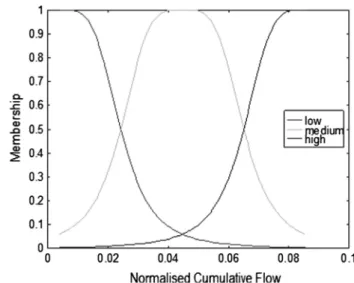
monsoon flows. The model is trained with 37 years of cumula-tive flows of different durations and checked with data of 12 years. Putting the cumulative flows at 10%, 20%and 30% of monsoon duration as inputs, the model was to predict cumulative monsoon flow at the end of the season. The gener-alized bell function is chosen as the membership function. The root mean square error (RMSE) in training and testing phases are 0.0058 and 0.0055 where as model efficiency (R2) for these phases are 0.998 and 0.999. The variation of training and test-ing errors (RMSE) with traintest-ing epochs are shown inFig. 3a. These figures indicate that the learning is almost complete at 475 epochs. The learned membership function is plotted in
Fig. 3b. This shows that each variable is attached with three qualifications, viz. ’’low’’, ’’medium’’ and ‘‘high’’.
The scatter plots and time series plots of modeled verses ac-tual cumulative flows inFigs. 3c–3freveal that the model can predict the monsoon flow at 100% duration of monsoon, with high accuracy.
The consequent parameters of the fuzzy inference system are shown inTable 2. The learned fuzzy if–then rules are
men-tioned inTable 3. The cumulative flow at 100% duration is gi-ven by the equation mentioned below theTable 2.
A second ANFIS model is developed to forecast the 100% cumulative inflows with only two inputs, namely, cumulative flows recorded at 10% and 20% of the duration of the monsoon. The total monsoon flow forecaster with two inputs uses generalized bell membership function, the parameters of which are mentioned inTable 4. With the inputs of cumulative flow at 10% and 20% of the duration of the monsoon, the predictor is to assess the flow at 100% monsoon duration.
The learned rules of ANFIS based monsoon flow predictor with two rules are shown in tables.Tables 4 and 5present the premise and consequent parameters, whileTable 6presents the fuzzy if–then rules. The forecasting rules are presented in Ta-ble 7. In this table, Zrefers to the cumulative flow at 100% duration of monsoon for a given year.
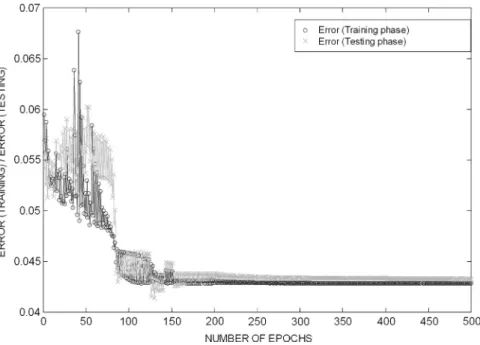
The minimum RMSE in training and testing phases of the model are 0.0428 and 0.041396. The efficiencies of the model are 0.919 in training and 0.955 in testing phases. The variation of RMSE is shown inFig. 4a. It is seen that the learning is al-most over after 275 epochs.
The graphical indicators of performance, such as the scatter plots and linear plot of actual and modeled cumulative nor-malized flows are shown inFigs. 4b–4ein training and testing phases of the model.
The landscape view of the decision from the ANFIS model shown inFig. 5presents the decision surface of the predicted standardized cumulative inflow in a given year, with the 10% standardized cumulative inflow and 20% standardized cumu-lative inflow as inputs to the Neuro-fuzzy model.
It is observed that the effect of the 10% cumulative flow is less prevalent, where as the 20% cumulative flow has a decisive impact on the total (100%) cumulative flow in the year under consideration. The above results clearly reveal that the models are well calibrated and the validation is also fit to be accept-able. Hence they can be used as good predictors of the cumu-lative monsoon flow at 100% duration of monsoon. The effectiveness of the model with three inputs (10%, 20% and 30% cumulative flows) is better than the model with two in-puts (10% and 20% cumulative flows), which matches with the natural observation. In cases, from administrative view point or from planning point of view, when it is required to predict the total flow in the very beginning of the monsoon, the model with two inputs can serve the purpose. This can later on be strengthened by the model with three inputs.
4. Analysis of runoff using GA-NLMR model
The relationship between run-off (Q(t)) with combination of control factors (H(t), H(t1), Q(t1)) is obtained using NLMR for month of June–October as given Table 8 along with Coefficient of Multiple Determination (R2).
The objective function is to maximize runoff which is given below: Maximize QðtÞ ð1Þ Subjected to constraints: ðHðtÞÞminHðtÞ ðHðtÞÞmax ðHðt1ÞÞminHðt1Þ ðHðt1ÞÞmax ðQðt1ÞÞminQðt1Þ ðQðt1ÞÞmax ð2Þ Figure 4d Scatter plot of actual versus modeled standardized
cumulative inflow.
Figure 4e Time series plot of actual versus modeled standardized cumulative inflow.
The suffixes minimum (min) and maximum (max) in Eq.(2)
show the lowest and highest value of rainfall (H(t)), penalty mate rainfall (H(t)1) and penalty mate runoff (Q(t)1) from period 2003–2007 for June–October.
Genetic Algorithm (GA) is used to obtain the optimum value of the control factors that maximizes the objective function. The rationale behind the use of genetic algorithm lies in the fact that it has the capability to find the global optimal parameter settings whereas the traditional optimization techniques are normally trapped at local optima. An important characteristic of genetic algorithm is the coding of variables that describes the problem. The most common coding method used in this work is binary code which transforms the variables to a binary string. As the problem has more than one variable, a multi-variable coding is constructed by concatenating as many single variable coding as the number of variables in the problem. Genetic Algorithm pro-cesses a number of solutions simultaneously. Hence, in the first step a population having P individuals is generated by pseudo random generators whose individuals represent a feasible solu-tion. This is a representation of solution vector in a solution space and is called initial solution. This ensures the search to be robust and unbiased, as it starts from wide range of points in the solution space. The population is then operated by three main operators; reproduction, crossover and mutation to create a new population of points. In the next step, individual members of the population are evaluated to find the objective function value.
The computational algorithm is implemented in Turbo C++ and run on an IBM Pentium IV machine. Different population size, probability of crossover and mutation are set and the maximum runoff is obtained. Number of genera-tion is varied till the output is conversed. Model developed by NLMR for month of June–October is then taken into GA model to obtain the maximum runoff as indicated in Ta-ble 9. It has been observed that at Population size of 30, prob-ability of crossover (0.5) and mutation (0.95), maximum runoff predicted by GA is for month of August.Figs. 6–10show the convergences of Maximum runoff with generation for different months. It has been observed that GA gives maximum runoff 49259.89 m3/s in the month of August at generation of at con-trol factor setting of 219.22 mm (H(t)), 219.05 mm (H(t1)) and 431.56 m3/s (Q(t1)).
4.1. Sensitivity analysis
Sensitivity analysis has been carried out for the months of June, July, August, September, and October with varying pop-ulation size, cross over and mutation probability at different levels, i.e. 1, 2, 3, 4 and 5. In the present work population var-iation has been taken for five different levels where as cross over and mutation has been considered for three different lev-els, to study the performance characteristics as shown in
Table 10.
Figure 5 The landscape view of the decision from the ANFIS model showing the predicted standardized cumulative flow in a given year, with the 10% standardized cumulative flow and 20% standardized cumulative flow as inputs into the model.
Table 8 Non-linear multiple regression.
Month Equation R2 June Q(t) = 993.75\H(t) 759.75\H(t 1) + 0.75\Q(t 1)48871.31 0.9640 July Q(t) = 1564.74\H(t) 1128.97\H(t 1) + 0.68\Q(t 1)91220.21 0.9491 August Q(t) = exp (0.33\H(t) + (6.88E 02).781)(1.7E5)\Q(t 1)76.78 0.9635 September Q(t) = 1540.92\H(t) 1147.15\H(t 1) + 0.71\Q(t 1)82539.71 0.9620 October Q(t) = 1043.49\H(t) 899.21\H(t 1) + 0.85\Q(t 1)30168.99 0.9786
Figure 6 Maximum runoff for the month of June.
Figure 7 Maximum runoff for the month of July.
Figure 8 Maximum runoff for the month of August.
Figure 9 Maximum runoff for the month of September.
Figure 10 Maximum runoff for the month of October.
Table 10 Control factor of GA parameters at different levels.
Level Population Cross over Mutation
1 10 0.1 0.1
2 30 0.5 0.5
3 50 0.9 0.95
4 70 5 90
Table 9 Maximum runoff found by GA.
Month Control factor Maximum runoffQ(t) June H(t) = 215.985 14210.58 H(t1) = 208.368 Q(t1) = 8915.532 July H(t) = 217.980 26265.89 H(t1) = 208.471 Q(t1) = 17273.230 August H(t) = 219.226 49259.89 H(t1) = 219.050 Q(t1) = 431.568 September H(t) = 216.954 21852.21 H(t1) = 209.557 Q(t1) = 14590.610 October H(t) = 214.908 12794.58 H(t1) = 209.258 Q(t1) = 8046.250
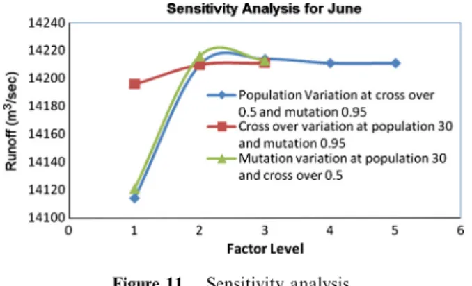
Similar patterns of performance characteristics has been observed for all the cases (June, July, August, September and October). Hence sensitive analysis graph for the month of June is presented here for reference. As shown inFig. 11, it has been observed that with increase in population size, run-off increases and ceases after population size of 30 at cross over of 0.5 and mutation probability of 0.95. It is observed fromFig. 11that at 0.1 cross over, runoff increases and there is no significant variation of runoff after increasing the cross over from 0.5 to 0.9 at population size of 30 and mutation probability of 0.95. With increase in mutation probability from 0.1 to 0.95 (at population size of 30 and crossover of 0.5), run-off increases and marginally drops after 0.5; and is found to be stabilized at 0.5 as shown inFig. 11.
5. Conclusions
In the present study non-linear multiple regression technique is employed for developing runoff rating models and runoff pre-diction models during monsoon period for the basin upstream of Basantpur gauging station of Mahanadi river, India. The re-sults of this study show that the models developed for mon-soon period can predict the runoff from the Mahanadi basin upstream of Basantpur site on a daily basis using historical information of water level. Hence these models can also be effectively utilized for interpolating missing data and for test-ing accuracy of other models. The results of Adaptive Neu-ro-fuzzy Inference System indicates the effectiveness of the model with three inputs (10%, 20% and 30% cumulative flows) is better than the model with two inputs (10% and 20% cumulative flows), which matches with the natural obser-vation. GA based evolutionary optimizer has been used to identify optimum process parameters in which runoff is maxi-mum. It is found that for the month of August runoff is max-imum as compared to other months.
References
[1] A.F. Atiya, S.M. El-Shoura, S.I. Shaheen, M.S. El-Sherif, A comparison between neural-network forecasting techniques – case study, river flow forecasting, IEEE Transactions on Neural Networks 10 (2) (1999) 402–409.
[2] R. Baratti, B. Cannas, A. Fanni, M. Pintus, G.M. Sechi, M. Toreno, Riverflow forecast for reservoir management through neural networks, Journal of Neuro Computing 55 (2003) 421–437. [3] A.A. Barreto-Neto, C.R.D.S. Filho, Application of fuzzy logic to the evaluation of runoff in a tropical watershed, Environmental Modelling & Software 23 (2008) 244–253.
[4] Y. Bar-Shalom, Stochastic Dynamic Programming, Caution and Probing, IEEE Transaction 26 (5) (1981) 1184–1195.
[5] J.C. Bertoni, C.S. Tucci, R.T. Clarke, Rainfall-based real-time flood forecasting, Journal of Hydrology 131 (1992) 131– 339.
[6] R.J.C. Burnash, R.L. Ferral, A. McGuire Richard, A Generalized Streamflow Simulation System-Conceptual Modelling for Digital Computers, Report, Joint Federal State River Forecast Center, National Water Service, Sacramento, Calif. Dept. of Water Resources, 1983.
[7] P. Carriere, S. Mohaghegh, R. Gaskari, Performance of a virtual runoff hydrograph system, Journal of Water Resources Planning and Management 122 (6) (1996) 421–427.
[8] A. El-Shafie, A. Noureldin, Generalized versus non-generalized neural network model for multi-lead inflow forecasting at Aswan High dam, Hydrology and Earth System Sciences Discussion 7 (5) (2010) 7957–7993.
[9] O. Faridah, N. Mahdi, Reservoir inflow forecasting using artificial neural network, International Journal of Physical Sciences 6 (3) (2011) 434–440.
[10] K. Fatima, A. Shaheen, Estimation of surface runoff for Tarbela reservoir, in: ICAST 2008, Proceedings of 2nd International Conference on Advances in Space Technologies, Space in the Service of Mankind, 4747695, 2008, pp. 103–106.
[11] L. Garrote, R.L. Bras, A distributed model for real-time flood forecasting using digital elevation models, Journal of Hydrology 167 (1995) 279–306.
[12] K.P. Georgakakos, G.F. Smith, On improved operational hydrologic forecasting - results from a WMO real-time forecasting experiment, Journal of Hydrology 114 (1990) 17–45.
[13] M. Hino, Prediction of flood and streamflow by modern control and stochastic theories, in: Proceedings 2nd International IAHR, Symposium of Stochastic Hydraulics, 1977, pp. 5-1–5-26.
[14] D.H. Hoggan, Computer assisted flood plain hydrology and hydraulics, McGraw Hill Publishing Company, New York, 1989.
[15] A. Jain, A. Kumar, An evaluation of artificial neural network technique for the determination of infiltration model parameters, Applied Soft Computing 6 (2006) 272–282. [16] W.P. James, C.G. Robinson, J.F. Bell, Radar assisted real-time
flood forecasting, Journal of Water Resources Planning and Management, ASCE 119 (1) (1993) 32–44.
[17] V.U. Joshi, D.T. Tambe, Estimation of infiltration rate, run-off and sediment yield under simulated rainfall experiments in upper Pravara basin, India, effect of slope angle and grass-cover, Journal of Earth System Science 119 (6) (2010) 763–773.
[18] P.K. Kitanidis, R.L. Bras, Real time forecasting with a conceptual hydrological model. 1 – analysis of uncertainty, Water Resources Research 16 (6) (1980) 1025–1033.
[19] U.C. Kothyari, Estimation of monthly runoff from small catchment in India, Hydrological Science Journal 40 (4) (1995) 533–541.
[20] U.C. Kothyari, R.J. Garde, V.R. Raju, Monthly runoff estimation for small catchments, Irrigation & Power 49 (3) (1992) 91–100.
[21] D. Mukherjee, N. Mansour, Estimation of flood forecasting errors and flow duration joint probabilities of excedance, Journal of Hydrology 122 (1996) 130–140.
[22] P.C. Nayak, K.P. Sudheer, K.S. Ramasastri, Fuzzy computing based rainfall–runoff model for real time flood forecasting, Hydrological Processes 19 (2005) 955–968.
[23] P.C. Nayak, K.P. Sudheer, D.M. Rangan, K.S. Ramasastri, A neuro-fuzzy computing technique for modeling hydrological time series, Journal of Hydrology 291 (1–2) (2004) 52–66.
[24] T.G. Nguyen, J.L. de Kok, M.J. Titus, A new approach to testing an integrated water systems model using qualitative scenarios, Environmental Modelling and Software 22 (11) (2007) 1557–1571. [25] H. Raman, N. Sunil Kumar, Multivariable modelling of water resources time series using artificial neural networks, Hydrological Sciences Journal 40 (2) (1995) 145–163.
[26] R. Remesan, M.A. Shamim, Runoff prediction using an integrated hybrid modelling scheme, Journal of Hydrology 372 (1–4) (2009) 48–60.
[27] S.B.K. Tan, L.H.C. Chua, E.B. Shuy, E.Y.-M. Lo, L.M. Lim, Performances of rainfall–runoff models calibrated over single and continuous storm flow events, Journal of Hydrologic Engineering 13 (7) (2008) 597–607.
[28] K. Thirumalaiah, M.C. Deo, River stage forecasting using artificial neural networks, Journal of Hydrologic Engineering 3 (1) (1998) 26–32.
[29] G. Tiron, S. Gosav, The July 2008 rainfall estimation from Barnova WSR-98 D radar using artificial neural network, Romanian Reports on Physics 62 (2) (2010) 405–413.
[30] A.S. Tokar, M. Markus, Precipitation–runoff modelling using artificial neural networks and conceptual models, Journal of Hydrologic Engineering 5 (2) (2000) 156–161.
[31] P.S. Yu, T.Y. Tseng, A model to forecast flow with uncertainty analysis, Hydrological Sciences Journal 41 (3) (1996) 327–344.