Mortgage Default in an Estimated Model of the U.S.
Housing Market
∗
Luisa Lambertini
†EPFL
Victoria Nuguer
‡Banco de M´
exico
Pinar Uysal
§Federal Reserve Bank of Richmond
May 1, 2016
Abstract
This paper models the housing sector, mortgages and endogenous default in a DSGE setting with nominal and real rigidities. We use data for the period 1981-2006 to estimate our model using Bayesian techniques. We analyze how an increase in risk in the mortgage market raises the default rate and spreads to the rest of the economy, creating a recession. In our model two shocks are well suited to replicate the subprime crisis and the Great Recession: the mortgage risk shock and the housing demand shock. Next we use our estimated model to evaluate a policy that reduces the principal of underwater mortgages. This policy is successful in stabilizing the mortgage market and makes all agents better off.
Keywords: Housing; Mortgage Default; DSGE model; Bayesian Estimation.
∗The views expressed herein are those of the authors and do not necessarily reflect those of Bank of Mexico, the Federal Reserve Bank of Richmond, or the Federal Reserve System.
†Ecole Polytechnique F´´ ed´erale de Lausanne, Chair of International Finance, Station 5, Odyssea ODY 2.05, CH-1015 Lausanne, Switzerland; telephone: +(41) 21 693 0050. E-mail: luisa.lambertini@epfl.ch.
‡Banco de M´exico, Dirreci´on General de Investigaci´on Econ´omica, 5 de Mayo 18, 06059 Ciudad de M´exico, M´exico. E-mail: vnuguer@banxico.org.mx.
§Federal Reserve Bank of Richmond, 502 S. Sharp Street, Baltimore, MD 21201, United States. E-mail: pinar.uysal@rich.frb.org.
1
Introduction
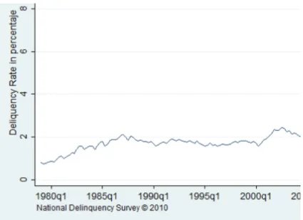
The latest financial crisis has its origins in the housing sector. There was an increase in the mortgage delinquency rate that put many financial institutions under distress. The bursting of the housing bubble in the United States made it difficult for borrowers to repay their loans. As a result, the seriously delinquent mortgage rate (more than 90 days past due and in foreclosure) increased from around 2% of total loans in 2006Q3 up to almost 10% in 2010Q1, as shown in Figure 1. Banks were forced to write down several hundred billions in bad loans. A credit crunch followed that caused the failure of several financial institutions. There was a decrease in the access to credit for households, house prices fell, and so did credit, consumption, and housing investment. The turmoil in the housing sector spread to the rest of the economy.
In this paper, we propose a model to analyze the transmission of an increase in mortgage default to the rest of the economy, the quantitative effects of the transmission and spillovers, and debt reduction policies that might mitigate these effects. First, we develop a comprehen-sive DSGE model with the housing sector, mortgages, and endogenous default and we estimate it using Bayesian techniques. Second, we use the estimated model to look at the effects of a reduction in mortgage payments.
This is a medium-sized model which builds on the work of Iacoviello and Neri (2010) and Forlati and Lambertini (2011). There are two types of households that differ in terms of their discount factor: patient households (lenders) save and lend to impatient ones (borrowers). Bor-rowers can take a loan pledging their houses as collateral. In Iacoviello and Neri’s equilibrium, mortgages are always repaid. We assume instead, like in Forlati and Lambertini, that the re-turns to housing are sensitive to both aggregate and idiosyncratic risk. The housing investment is subject to a risk shock that determines the value of the collateral. If the value of the collateral after the shock is lower than the repayment of the loan, the borrower defaults on the mortgage. Lenders can observe the realized return only after paying an auditing cost. The participation constraint implied by the financial contract makes the rate of default on mortgages and the external finance premium countercyclical.
The entrance of subprime borrowers in the U.S. mortgage market between 2000 and 2006 is captured with an increase in the standard deviation of idiosyncratic housing investment risk, which we refer to as mortgage risk shock. Because of this risk, some borrowers find themselves
Figure 1: Delinquency Rate in Percentage Points, United States, 1979Q4-2010Q1
in a negative equity trap and default on their mortgages. The ensuing fall in house prices pushes more mortgages underwater and triggers a credit crunch that reduces aggregate demand for housing and non-durable goods alike. The economy experiences a recession. We estimate the model with U.S. data for the time period 1981Q1-2006Q4 using Bayesian techniques.
The Financial Stability Act of 2009 launched Making Home Affordable (MHA) in response to the increase in the mortgage default rate. Among other programs the Home Affordable Modi-fication Program (HAMP) was started. The objectives of this program are to help households to avoid foreclosure, to stabilize the U.S. housing market, and to improve the economy. It con-sists of loan modifications on the mortgage debt. The loan modifications are either permanent reductions in the mortgage payments through a lowering of monthly payments or a reduction in the mortgage rate.
In line with these events, we use the estimated model for policy evaluation. We study a re-duction in the loan payment that writes off the underwater part of mortgages. We find that this policy is effective in stabilizing the mortgage market and mitigating the macroeconomic effects of mortgage risk shocks. For housing demand shocks, the policy stabilizes the mortgage market but its effect on the aggregate economy is limited.
Following the work of Kiyotaki and Moore (1997), Iacoviello (2005) and Iacoviello and Neri (2010), we introduce collateral constraints in a model with housing to analyze sources and
con-sequences of fluctuations in the U.S. housing sector. In particular, Iacoviello (2005) develops and estimates a monetary business cycle model with nominal loans and durable goods used as collateral. The main features of this framework are: (1) collateral constraint tied to real estate values (as in Kiyotaki and Moore (1997)) and (2) nominal debt. These features result in a financial accelerator mechanism. Iacoviello (2005) estimates this model using U.S. data from 1974Q1 to 2003Q2. He finds that there are positive feedback effects from shocks on housing preferences to non-housing consumption stemming from the collateral constraint.
Iacoviello and Neri (2010) develop a DSGE model of the U.S. economy that includes the housing sector and estimate it using Bayesian techniques. The core of Iacoviello and Neri’s framework, and that of ours, is a dynamic equilibrium model with neoclassical assumptions and nominal and real rigidities, as the seminal works of Christiano, Eichenbaum and Evans (2005) and Smets and Wouters (2007). These papers do not model the housing sector explic-itly but they fit the U.S. data well. The housing features in Iacoviello and Neri’s work builds on Iacoviello (2005). Their model is characterized by sectorial heterogeneity, as in Davis and Heathcote (2005). It features the housing sector which produces new homes using capital, labor, and land, and the non-housing sector that produces consumption goods and business investment using capital and labor. On the demand side, housing can be used as collateral for borrowing, as in Iacoviello (2005). Iacoviello and Neri find that housing demand and sup-ply shocks explain about one-quarter of the volatility of both housing investment and housing prices. They show that housing market spillovers to consumption and business investment have become more important over time. Our model allows for endogenous default on mortgages and we quantify its role in the transmission.
The paper is organized as follows. Section 2 describes the model. Section 3 discusses the methodology. Section 4 documents the characteristics of the model with the estimated param-eters. In Section 5 we look at the sources of business cycle fluctuation. In Section 7 we study the effects of debt reduction. Section 8 concludes.
2
Model
Our model has two sectors, durable and non-durable goods; two types of households, patient (lender) and impatient (borrower); and endogenous default on mortgage contracts. In
equilib-rium, some mortgages are defaulted. We assume that the returns to housing are sensitive to both aggregate and idiosyncratic risks and that lenders can observe the realized return only after paying an auditing cost. The participation constraint implied by the financial contract makes the rate of default on mortgages and the external finance premium countercyclical. For ease of comparison, we keep the same notation as Iacoviello and Neri (2010).
2.1
Households
There is a continuum of households of measure 1. Households differ in terms of their discount factor: patient households (lenders) save and lend to impatient ones (borrowers).
2.1.1 Lenders
Lenders maximize their lifetime utility function:
maxE0 ∞ X t=0 (βGc)tzt Γcln(ct−ct−1) +jtlnht− τt 1 +η n1+c,tξ+n1+h,tξ 1+η 1+ξ , (1)
where β is the discount factor, ct is consumption of non-durable goods, ht is consumption of
housing services, nc,t and nh,t are hours in the non-durable goods sector and housing sector,
respectively. The variableszt,jt, andτtdenote the shocks to intertemporal preferences, housing
preferences, and labor supply.1 The parameter measures habit persistence, ηis the inverse of the Frisch labor supply elasticity, and ξ accounts for the imperfect substitution of hours in the
non-durable and housing sectors. Consumption grows at the rate Gc on the balanced growth
path and Γc= (Gc−)/(Gc−βGc) allows marginal utility of consumption to be equal to 1/c
in the steady state.
Lenders maximize their utility subject to their budget constraint:
ct+qtht+bt+ kc,t Ak,t + X i=h,b ki,t+pl,tlt= Rt−1bt−1 πt +qt(1−δh)ht−1+ X i=c,h wi,tni,t Xwi,t (2) +[Rh,tzh,t+ 1−δk,h]kh,t−1+ Rc,tzc,t+ 1−δk,c Ak,t kc,t−1+ (pl,t+Rl,t)lt−1+pb,tkb,t +Divt−φt− a(zc,t)kc,t−1 Ak,t −a(zh,t)kh,t−1.
Lenders choose non-durable goods ct, housing services ht, hours nc,t and nh,t, land lt, capital
in the consumption sector kc,t, capital kh,t and intermediate inputs kb,t in the housing sector,
lendingbt(borrowing if positive), and capital utilization rateszc,t andzh,t. The price of housing
relative to consumption is qt, the price for intermediate inputs ispb,t, and the price of land is
pl,t. Ak,t is an investment-specific technology shock. Rt−1 is the nominal return on the riskless
bond and πt = Pt/Pt−1 is the money inflation rate in the non-durable sector. Real wages are wc,t and wh,t, real rental rates are Rc,t and Rh,t, and depreciation rates are δk,c and δk,h. There
is monopolistic competition in the labor market, and Xwc,t and Xwh,t represent the markup
between the wage paid by the wholesale firm and the wage paid to the households. Final goods firms and labor unions pay lump-sum profits Divt;φt is the capital adjustment cost, and a(zi,t)
is the convex cost of setting capital utilization rate to zi,t, which are specified in Appendix B.
2.1.2 Borrowers
Borrowers maximize their lifetime utility function:
maxE0 ∞ X t=0 (β0Gc)tzt " Γ0cln(c0t−ct0−1) +jtlnh0t− τt 1 +η0 (n0c,t)1+ξ0 + (n0h,t)1+ξ0 1+η0 1+ξ0 # , (3)
subject to their budget constraint:
c0t+qth0t+ [1−Ft(¯ωt)]Rz,tbt−1 =bt+ X i=c,h w0i,tn0i,t Xwi,t0 + (1−δh)[1−Gt(¯ωt)]qth 0 t−1+Div 0 t. (4)
Variables and parameters with a prime refer to the borrowers who have a lower discount rate than lenders (β0 < β). Rz,t is the state-contingent interest rate that non-defaulting borrowers
pay at time t on the loans bt−1 taken at time t−1; it is an adjustable interest rate determined
after the realization of the shocks and it satisfies the participation constraint of the lenders. A fraction of borrowers default on their mortgages and, as a result, lenders pay the monitoring cost µand seize a fractionGt(¯ωt) of the borrowers’ housing stock. The fraction of loans that is
repaid to the lenders is denoted by [1−Ft(¯ωt)]. Div
0
t are specified in Appendix B.
Each household consists of many members who are ex-ante identical. The household decides how much to invest in housing and ¯ωt, the threshold for default. Total housing investment is
the lender and then the idiosyncratic shock ωi
t+1 is realized. The shock defines the ex-post
value of the house ωi
t+1qt+1h0t. This captures the idea that housing investment is risky. The
idiosyncratic shock is i.i.d. across the household members and log-normally distributed with the cumulative distribution function Ft+1(ωit+1). The expected value of the ωit+1 is equal to
1 in every period, so there is no aggregate uncertainty. We assume that housing investment riskiness can change over time: the standard deviation σω,t of lnωti is subject to an exogenous
shock.
Once the idiosyncratic shock is realized, the borrower decides whether to default on the mortgage or not. The borrower defaults if the idiosyncratic shock is such that the value of the house is lower than mortgage repayment. This implicitly defines the threshold ¯ωt+1:
¯
ωt+1(1−δh)qt+1h0tπt+1 =Rz,t+1 bt. (5)
Loans that experience an idiosyncratic shock greater than this threshold value are repaid at the contractual rate Rz,t+1 and loans that experience idiosyncratic realizations lower than this
threshold value are underwater and are defaulted on. The random variable ωi
t+1 is observed by
the members of the household but lenders can only observe it after paying a cost. Then, lenders pay the monitoring costµand seize the collateral on the loan. This makes the borrowers truth-fully reveal their idiosyncratic shock. Borrowers that default lose their housing stocks. There is perfect consumption insurance among household members so that non-durable consumption and housing investment are ex post equal across members of the household.
We assume a one-period mortgage contract as in Bernanke, Gertler and Gilchrist (1999). Lenders demand the gross rate of return Rt which is predetermined and not state contingent.
The participation constraint of the lenders is
Rtbt = Z ω¯t+1 0 ωt+1(1−µ)(1−δh)qt+1h0tπt+1ft+1(ω)dω+ Z ∞ ¯ ωt+1 Rz,t+1btft+1(ω)dω, (6)
wheref(ω) is the probability density function ofω. Remember thatωis subject to an exogenous shock to its standard deviation, making it time variant. The return on total loans consists of two parts: the housing stock net of monitoring costs and depreciation of the defaulting borrowers (first-term on the right-hand side of 6), and the repayment by the non-defaulting borrowers
(second-term on the right-hand side of 6). After the idiosyncratic and aggregate shocks are realized, the threshold value ¯ωt and the state-contingent mortgage rate Rz,t are determined.
The participation constraint holds state by state.
As in Forlati and Lambertini (2011) we define the expected value of the idiosyncratic shock for those who default multiplied by the probability of default as
Gt+1(¯ωt+1)≡
Z ω¯t+1
0
ωt+1ft+1(ω)dω (7)
and the expected share of housing value, gross of monitoring costs, that goes to lenders as,
Γt+1(¯ωt+1)≡ω¯t+1
Z ∞
¯
ωt+1
ft+1(ω)dω+Gt+1(¯ωt+1). (8)
Then, the participation constraint, Equation (6), can be rewritten as
Rtbt = [Γt+1(¯ωt+1)−µGt+1(¯ωt+1)] (1−δh)qt+1h0tπt+1, (9)
where the loan-to-value ratio is
[Γt+1(¯ωt+1)−µGt+1(¯ωt+1)]. (10)
We derive Equation (9) in Appendix C. We also show another way of writing the borrowers’ budget constraint, Equation (4). Equation (9) states that the borrower can borrow, bt, up
to a fraction of the future value of the house. The loan-to-value ratio is such fraction; it is determined endogenously and it is time-varying.
Borrowers maximize their utility (3) subject to the budget constraint (4) and the borrowing constraint (9). They choose c0t, h0t, bt,n0h,t, n
0
c,t, and ¯ωt+1.
We follow Bernanke et al. (1999) and Forlati and Lambertini (2011) to specify the idiosyncratic risk in the housing sector. The shock ω is distributed log-normally:
lnωt ∼N −σ 2 ω,t 2 , σ 2 ω,t . (11)
2.2
Firms
There are competitive flexible price wholesale firms that produce non-durable goods and hous-ing ushous-ing two technologies. There is also a final good firm in the non-durable sector which operates under monopolistic competition.
Wholesale firms hire labor and capital services and buy intermediate goods to produce whole-sale goods Yt and new houses IHt to maximize their profits
Yt Xt +qtIHt− " X i=c,h
(wi,tni,t+wi,t0 n
0
i,t+Ri,tzi,tki,t−1) +Rl,tlt−1+pb,tkb,t
#
, (12)
where the production technologies are:
Yt = h Act nαctn0ct1−αi 1−µc (zctkct−1) µc , (13) IHt = h Aht nαhtn0ht1−αi 1−µh−µb−µl (zhtkht−1)µhkbtµbl µl t−1. (14) Xt is the markup of final good relative to wholesale non-durable good. Non-durable goods are
produced with labor and capital as in (13). New houses are produced with labor, capital, land, and intermediate input kb as in (14). Act and Aht denote the productivities in the non-durable
and housing sectors.
2.3
Nominal Rigidities and Monetary Policy
There is price rigidity in the non-durable sector and wage rigidities in the non-durable and housing sectors. We assume monopolistic competition at the retail level and price stickiness `
a la Calvo (Calvo, 1983). Retailers buy wholesale goods Yt from wholesale firms at the price
Pw
t in a competitive market, differentiate the goods at no cost, and sell them at a markup
Xt = Pt/Ptw over the marginal cost. The CES aggregates of these goods are converted back
into homogeneous consumption and investment goods by households. Each period, a fraction 1−θπ of retailers set prices optimally, while a fraction θπ cannot do so, and index prices to the previous period inflation rate with an elasticity equal to ιπ . These assumptions deliver the
following consumption sector Phillips curve: lnπt−ιπlnπt−1 =βGc(Etlnπt+1−ιπlnπt)−επln Xt X +up,t, (15)
where επ = (1−θπ)(1−βGcθπ)/θπ and up,t is a cost shock.
Wage setting is similar to price setting. Unions receive homogeneous labor supply from borrow-ers and lendborrow-ers. Then they differentiate the labor services and set wages `a la Calvo. Wholesale labor packers buy these labor services and assemble them into nc, nh, n0c, and n
0
h. Wholesale
firms hire labor from these packers. Under Calvo pricing with partial indexation to past infla-tion, the pricing rules set by the union imply four wage’s Phillips curves that are isomorphic to the price’s Phillips curve. These equations are in Appendix B.
To close the model, we assume that the central bank sets the interest rate Rt according to a
Taylor rule that responds to past interest rate, inflation, and GDP growth:
Rt = (Rt−1)rR πrπ t GDPt GcGDPt−1 rY ¯ rr 1−rR uRt st , (16)
where ¯rris the steady-state interest rate,uRt is i.i.d. monetary policy shock, andstis persistent
inflation target shock.
2.4
Equilibrium
The equilibrium in the goods market is as follows:
Ct+ IKc,t Ak,t +IKh,t+kb,t=Yt−φt, (17) where Ct = ct +c 0
t is the aggregate consumption, IKc,t = kc,t − (1 − δk,c)kc,t−1, IKh,t =
kh,t−(1−δkh)kh,t−1, and φt is described in Appendix B.
New houses are produced in the housing market:
ht+h 0 t−(1−δh) h ht−1+h 0 t−1(1−µGt(¯ωt)) i =IHt. (18)
Loan market also clears. Total land is fixed and normalized to one. The shocks are described in Appendix B.
2.5
Trends and Balanced Growth
To complete the model, we allow for different productivity trends in the consumption, business, and residential sector. The processes that they follow are:
lnAc,t=tln (1 +γAC) + lnZc,t, where lnZc,t =ρAClnZc,t−1+uC,t;
lnAh,t =tln (1 +γAH) + lnZh,t, where lnZh,t =ρAHlnZh,t−1+uH,t;
lnAk,t=tln (1 +γAK) + lnZk,t, where lnZk,t =ρAKlnZk,t−1+uK,t.
The innovations are uC,t,uH,t, anduK,t and they have mean zero and standard deviationsσAC,
σAH, and σAK. The shocks are serially uncorrelated. The parameters γAC, γAH, and γAK are
the net growth rates of technology for each of the sectors. We estimate the last six parameters. A balance growth path exists. We follow Iacoviello and Neri (2010) to define the growth rates for the real variables as
GC =GIKh =Gq×IH = 1 +γAC+ µC 1−µC γAK; (19) GIKc= 1 +γAC + 1 1−µC γAK; (20) GIH = 1 + (µh+µb)γAC+ µc(µh+µb) 1−µc γAK + (1−µh−µl−µb)γAH; (21) Gq = 1 + (1−µh−µb)γAC+ µc(1−µh−µb) 1−µc γAK−(1−µh−µl−µb)γAH. (22)
3
Parameter Estimates
3.1
Methods and Data
We take the linearized version of the equations around the balanced growth path and estimate the model with Bayesian methods. The chosen prior distributions are discussed in Section 3.3, and we estimate the posterior distributions using the Metropolis-Hastings algorithm. We have eleven observables: loan-to-value ratio, real consumption, real residential investment, real
business investment, real house prices, nominal interest rates, inflation, hours and wage inflation in the consumption sector, hours and wage inflation in the housing sector. The variables are explained in Appendix A. We measure the loan-to-value ratio following Boz and Mendoza (2014) and define it as net credit market assets of households divided by the value of residential land from Davis and Heathcote (2007).
We use quarterly data for the United States from 1981Q1 until 2006Q4, to exclude the financial crisis period. However, we also experiment with the data until 2008Q4, before the nominal interest rate reached the zero lower bound. We plot the data that we use in the estimation in Figure E.1.
3.2
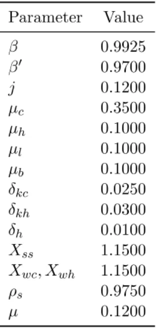
Calibrated Parameters
We present the parameters we calibrate in Table 1 and we follow Iacoviello and Neri (2010).2 The discount rate for borrowers isβ = 0.9925, and the discount rate for lenders isβ0 = 0.9700. The weight on housing in the utility function j is equal to 0.12. The share of capital in the non-durable goods production µc is set to 0.35. In the housing production the capital shareµh,
the share of land µl, and the share of intermediate goodsµb are all set to 0.1.
We set the depreciation rates for capital in the non-durable goods sector δkc = 0.025, capital
in the housing sector δkh = 0.03, and the depreciation in the housing sector δh = 0.01. The
steady-state markups are equal to 15 percent, so we fix Xss, Xwc, and Xwh at 1.15. The
autocorrelation parameter for the cost shock ρsis fixed at 0.975. Finally, we set the monitoring
cost µ equal to 0.12 as in Forlati and Lambertini (2011).
3.3
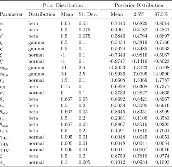
Prior and Posterior Distributions
We present our prior distributions in Tables 2 and 3. Most of the priors have the same distri-butions as in Iacoviello and Neri (2010). The only difference is the parameters that specify the autoregressive part of the shocks i.e. ρ’s. We set the prior mean of these parameters to 0.5.
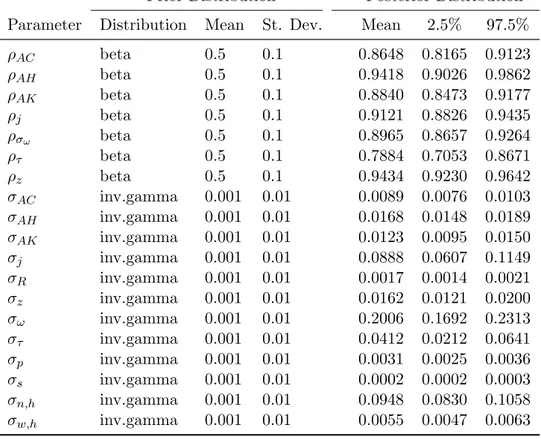
We specify a normal distribution for the mean of standard deviation of idiosyncratic shocks in the housing sector ¯σω. The idiosyncratic shock itself is specified similar to the other shocks in
the model, i.e. the autoregressive parameter has a beta distribution with mean equal to 0.5 and 2See Iacoviello and Neri (2010) for the details of the calibration.
Parameter Value β 0.9925 β0 0.9700 j 0.1200 µc 0.3500 µh 0.1000 µl 0.1000 µb 0.1000 δkc 0.0250 δkh 0.0300 δh 0.0100 Xss 1.1500 Xwc, Xwh 1.1500 ρs 0.9750 µ 0.1200
Table 1: Calibrated Parameters
standard deviation equal to 0.1, and the standard deviation has an inverse gamma distribution with mean 0.001 and a standard deviation of 0.01.
Tables 2 and 3 show the posterior distribution of the parameters and the shock processes, respectively. Figures E.9 to E.13 in Appendix E present the plots of the prior and the posterior distributions.
4
Properties of the Estimated Model
4.1
Impulse Responses
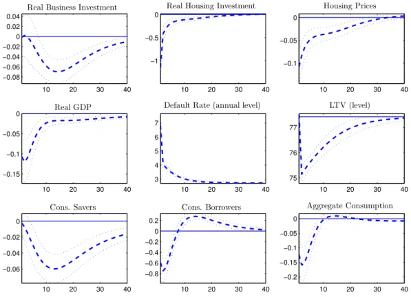
Mortgage Risk Shock.- Figure 2 plots impulse responses to the estimated mortgage risk shock.3
The magnitude of the shock is equal to the mode of the estimated distribution, σω = 0.1927.
The mortgage risk shock is captured by an unanticipated increase inσω,t, the standard deviation
of the distribution of the idiosyncratic housing investment risk. An increase in mortgage risk implies an increase in the default rate of borrowers and an increase in the monitoring cost. Lenders require a higher interest rate from the borrowers who do not default on their loans, because the participation constraint needs to be satisfied, and the external finance premium increases. Additionally, the loan-to-value ratio of the borrowers decreases which in turn leads to
Prior Distribution Posterior Distribution Parameter Distribution Mean St. Dev. Mean 2.5% 97.5% α beta 0.65 0.05 0.7440 0.6826 0.8014 beta 0.5 0.075 0.4001 0.3182 0.4841 0 beta 0.5 0.075 0.5846 0.4764 0.6897 η gamma 0.5 0.1 0.5434 0.3819 0.7166 η0 gamma 0.5 0.1 0.5024 0.3485 0.6563 ξ normal -1 0.1 -0.7343 -0.9816 -0.5067 ξ0 normal -1 0.1 -0.9747 -1.1416 -0.8023 φk,c gamma 10 2.5 14.3053 11.3023 17.6198 φk,h gamma 10 2.5 10.9936 7.0095 14.9590 rπ normal 1.5 0.1 1.6608 1.5369 1.7787 rR beta 0.75 0.1 0.6828 0.6308 0.7377 rY normal 0 0.1 0.3739 0.2827 0.4665 θπ beta 0.667 0.05 0.8692 0.8421 0.8967 ιπ beta 0.5 0.2 0.5039 0.3090 0.6910 θw,c beta 0.667 0.05 0.8645 0.8351 0.8999 ιw,c beta 0.5 0.2 0.2381 0.1109 0.3583 θw,h beta 0.667 0.05 0.8867 0.8516 0.9205 ιw,h beta 0.5 0.2 0.4491 0.1810 0.7061 γAC normal 0.005 0.01 0.0048 0.0045 0.0051 γAH normal 0.005 0.01 0.0048 0.0041 0.0054 γAK normal 0.005 0.01 0.0011 0.0007 0.0016 ζ beta 0.5 0.2 0.8759 0.7818 0.9774 ¯ σω normal 0.1 0.005 0.1012 0.0934 0.1093
Prior Distribution Posterior Distribution Parameter Distribution Mean St. Dev. Mean 2.5% 97.5% ρAC beta 0.5 0.1 0.8648 0.8165 0.9123 ρAH beta 0.5 0.1 0.9418 0.9026 0.9862 ρAK beta 0.5 0.1 0.8840 0.8473 0.9177 ρj beta 0.5 0.1 0.9121 0.8826 0.9435 ρσω beta 0.5 0.1 0.8965 0.8657 0.9264 ρτ beta 0.5 0.1 0.7884 0.7053 0.8671 ρz beta 0.5 0.1 0.9434 0.9230 0.9642 σAC inv.gamma 0.001 0.01 0.0089 0.0076 0.0103 σAH inv.gamma 0.001 0.01 0.0168 0.0148 0.0189 σAK inv.gamma 0.001 0.01 0.0123 0.0095 0.0150 σj inv.gamma 0.001 0.01 0.0888 0.0607 0.1149 σR inv.gamma 0.001 0.01 0.0017 0.0014 0.0021 σz inv.gamma 0.001 0.01 0.0162 0.0121 0.0200 σω inv.gamma 0.001 0.01 0.2006 0.1692 0.2313 στ inv.gamma 0.001 0.01 0.0412 0.0212 0.0641 σp inv.gamma 0.001 0.01 0.0031 0.0025 0.0036 σs inv.gamma 0.001 0.01 0.0002 0.0002 0.0003 σn,h inv.gamma 0.001 0.01 0.0948 0.0830 0.1058 σw,h inv.gamma 0.001 0.01 0.0055 0.0047 0.0063
Table 3: Prior and Posterior Distribution of Shock Processes
a tightening of the borrowing constraint of the borrowers. The worsening of financial conditions leads borrowers to cut back on non-durable consumption, housing investment, and loans. The housing demand of borrowers falls substantially; this drives the fall in house prices. Savers, who are consumption smoothers, can take advantage of the lower prices and increase housing demand. Nevertheless, the large drop in the housing demand of borrowers dominates. The consumption of lenders falls less than the consumption of borrowers because the borrowers bear all the risk in this type of contract. Savers also reduce lending due to lower interest rates. Overall, total consumption and output fall. Business investment falls slightly.
The wages in both sectors are lower both for borrowers and lenders. Wages for borrowers fall more than for lenders. Savers and borrowers work less.
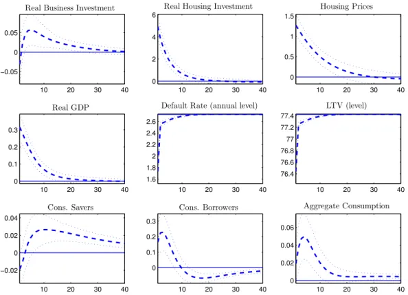
Housing Preference Shock.- Next, we analyze impulse responses to a housing preference shock in Figure 3.4 It is, as Iacoviello and Neri (2010) call it, a housing demand shock. A higher
housing demand leads to an increase in housing prices and in housing investment. The collateral 4Figure E.3 in Appendix E plots additional variables.
10 20 30 40 −0.08 −0.06 −0.04 −0.02 0 0.02 0.04
Real Business Investment
10 20 30 40
−1 −0.5 0
Real Housing Investment
10 20 30 40 −0.1 −0.05 0 Housing Prices 10 20 30 40 −0.15 −0.1 −0.05 0 Real GDP 10 20 30 40 3 4 5 6 7
Default Rate (annual level)
10 20 30 40 75 76 77 LTV (level) 10 20 30 40 −0.06 −0.04 −0.02 0 Cons. Savers 10 20 30 40 −0.8 −0.6 −0.4 −0.2 0 0.2 Cons. Borrowers 10 20 30 40 −0.2 −0.15 −0.1 −0.05 0 Aggregate Consumption
Figure 2: Impulse Responses to Mortgage Risk Shock
Dashed lines represent the mean of the posterior impulse responses; dotted lines indicate the 2 standard deviations confidence intervals.
capacity of the borrowers increases, and the wages for borrowers in both sectors also increase and they work more. These together allow the borrowers to consume more and to demand more housing. The default rate of the borrowers and the monitoring costs of the lenders are lower. Lenders require a lower external finance premium. The nominal interest rate is higher and lenders give out more loans. Savers decrease housing demand and consumption. Aggregate consumption increases because it is driven mainly by the borrowers’ non-durable consumption.
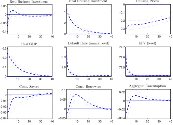
Housing Technology Shock.- Impulse responses to a housing technology shock are presented in Figure 4.5 A positive shock to housing technology results in higher housing investment and
lower housing prices. The fall in house prices decreases the collateral capacity of the borrowers. The default rate is higher, so are the monitoring costs and the external finance premium (not on impact because the risk free rate of return is predetermined). Lenders cut back their loans. They increase their housing demand and decrease their non-durable good consumption. Borrowers consume less non-durable goods.
10 20 30 40 −0.05
0 0.05
Real Business Investment
10 20 30 40
0 2 4 6
Real Housing Investment
10 20 30 40 0 0.5 1 1.5 Housing Prices 10 20 30 40 0 0.1 0.2 0.3 Real GDP 10 20 30 40 1.6 1.8 2 2.2 2.4 2.6
Default Rate (annual level)
10 20 30 40 76.4 76.6 76.8 77 77.2 77.4 LTV (level) 10 20 30 40 −0.02 0 0.02 0.04 Cons. Savers 10 20 30 40 0 0.1 0.2 0.3 Cons. Borrowers 10 20 30 40 0 0.02 0.04 0.06 Aggregate Consumption
Figure 3: Impulse Responses to Housing Preference Shock
Dashed lines represent the mean of the posterior impulse responses; dotted lines indicate the 2 standard deviations confidence intervals.
Savers’ wages in the housing sector go up and they work more; their wages in the non-durable goods sector decrease and they work less (on impact). Borrowers’ wages in the housing sector also go up and so do hours; in the consumption sector they move in a different direction. Total hours of savers and borrowers increase in the housing sector and decrease in the non-durable sector; investment in the different sectors co-moves with total hours. More resources go into the durable sector. Aggregate output in the non-durable sector falls. Overall, there is an increase in housing and real GDP goes up.
An interesting characteristic of the impulse responses is the high persistence of the housing prices to the estimated shock; this is due to the high posterior mean of the autocorrelation parameter of the housing technology shock, ρAH = 0.9474.6
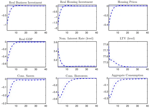
Monetary Policy Shock.- Figure 5 plots the impulse responses to an i.i.d. monetary policy
shock.7 The nominal interest rate goes up. Non-durable goods consumption, real business
and housing investment fall. Housing investment falls the most and is followed by business 6However, our estimated value is lower than Iacoviello and Neri’s,ρ
AH = 0.997, prompting a faster return
to the steady-state.
10 20 30 40 −0.1
−0.05 0 0.05
Real Business Investment
10 20 30 40
0 2 4
Real Housing Investment
10 20 30 40 −0.3 −0.2 −0.1 0 Housing Prices 10 20 30 40 0 0.1 0.2 0.3 Real GDP 10 20 30 40 2.8 2.9 3
Default Rate (annual level)
10 20 30 40 77.5 77.6 77.7 LTV (level) 10 20 30 40 −0.04 −0.03 −0.02 −0.01 0 Cons. Savers 10 20 30 40 −0.05 0 0.05 0.1 Cons. Borrowers 10 20 30 40 −0.04 −0.02 0 0.02 Aggregate Consumption
Figure 4: Impulse Responses to Housing Technology Shock
Dashed lines represent the mean of the posterior impulse responses; dotted lines indicate the 2 standard deviations confidence intervals.
investment and consumption, as in Iacoviello and Neri (2010). The consumption of savers falls because they are consumption smoothers. Consumption of borrowers drops due to two reasons. First, credit is more expensive. Second, the price of consumption goods falls and real debt is higher. Borrowers also have to reduce housing demand and hours worked. There is a negative wealth effect for the borrowers.
Total demand in the housing sector falls and housing prices drop, too. More borrowers default: for a larger fraction of members of the households the value of their house is lower than the value of their debt. Monitoring costs increase and so does the interest rate that borrowers pay. Lenders substitute loans with housing demand. The loan-to-value ratio increases, as expected. As aggregate demand falls, the wages in all sectors go down and both borrowers and lenders work less.
4.2
Business Cycle Properties
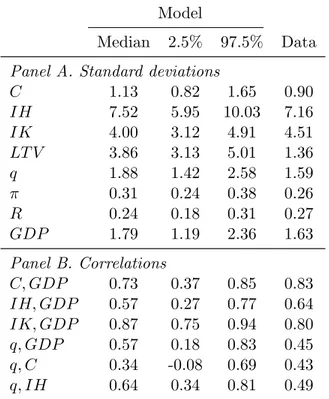
In Table 4 we present the business cycle statistics of our estimated model. Panel A reports the standard deviations, and Panel B reports the correlations. All standard deviations of the data
10 20 30 40 −1
−0.5 0
Real Business Investment
10 20 30 40 −2 −1.5 −1 −0.5 0
Real Housing Investment
10 20 30 40 −0.4 −0.2 0 Housing Prices 10 20 30 40 −0.6 −0.4 −0.2 0 Real GDP 10 20 30 40 3.2 3.4 3.6
Nom. Interest Rate (level)
10 20 30 40 77.5 77.6 77.7 77.8 LTV (level) 10 20 30 40 −0.3 −0.2 −0.1 0 Cons. Savers 10 20 30 40 −0.6 −0.4 −0.2 0 Cons. Borrowers 10 20 30 40 −0.3 −0.2 −0.1 0 Aggregate Consumption
Figure 5: Impulse Responses to Monetary Policy Shock
Dashed lines represent the mean of the posterior impulse responses; dotted lines indicate the 2 standard deviations confidence intervals.
are within the 95% of the probability interval computed from the model. The correlations of the variables are also well-replicated by our model.
5
Sources of Business Cycle Fluctuations
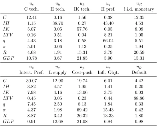
In Table 5, we present results from the forecast error variance decomposition. We find that housing demand (housing preference) shocks explain more than half of the variance in house prices. However, housing supply (housing technology) does not explain much of the variation in house prices. Each of these shocks explains more than a third of housing investment. Technology shocks in the non-durable sector explain investment in that sector.
Mortgage risk shocks explain about 88% of the variation in loan-to-value ratio, however it explains little of the other variables. We are adding one observed variable and one shock, and the shock explains the variables. However, our estimation does not include the crisis period and therefore does not capture the transmission of shocks from the mortgage market to the rest of the economy. In fact, the loan-to-value ratio and the default rate fluctuate little at business
Model
Median 2.5% 97.5% Data Panel A. Standard deviations
C 1.13 0.82 1.65 0.90 IH 7.52 5.95 10.03 7.16 IK 4.00 3.12 4.91 4.51 LT V 3.86 3.13 5.01 1.36 q 1.88 1.42 2.58 1.59 π 0.31 0.24 0.38 0.26 R 0.24 0.18 0.31 0.27 GDP 1.79 1.19 2.36 1.63 Panel B. Correlations C, GDP 0.73 0.37 0.85 0.83 IH, GDP 0.57 0.27 0.77 0.64 IK, GDP 0.87 0.75 0.94 0.80 q, GDP 0.57 0.18 0.83 0.45 q, C 0.34 -0.08 0.69 0.43 q, IH 0.64 0.34 0.81 0.49
Table 4: Business Cycle Properties of the Model
frequency until 2007.
Consumption is mainly driven by inter-temporal preferences and cost-push shocks; output is driven by technology shocks in the non-durable sector and cost-push shocks. In Figure E.8 in the Appendix, we show the visual representation of the forecast error variance decomposition for the loan-to-value ratio.
As we expressed in Equations (19) to (22), business investment, residential investment, and consumption have different trends. We estimate these trends and we compare them with the data. Figure 6 shows the results. In line with the data, we find that real business investment has a faster technological progress than real consumption and real residential investment. The lower technological progress in the construction sector explains the trend in real house prices. One of the reasons for the increase in house prices is the price of land which is a factor that limits the construction of new homes. We present robustness checks in Appendix D.
uc uh uk uj uR
C tech. H tech. IK tech. H pref. i.i.d. monetary
C 12.41 0.16 1.56 0.38 12.35 IH 1.15 38.70 0.27 43.40 4.53 IK 5.07 0.05 57.76 0.05 8.09 LT V 0.16 0.51 0.04 8.21 1.05 q 4.43 3.18 0.58 66.04 5.51 π 5.01 0.06 1.13 0.25 1.94 R 4.68 1.91 15.31 3.79 20.59 GDP 10.78 3.67 21.85 5.90 15.31 uz uτ up us uω¯ Intert. Pref. L supply Cost-push Infl. Objt. Default
C 30.07 12.90 19.74 6.01 4.42 IH 3.82 4.57 1.95 1.41 0.20 IK 7.98 4.16 13.06 3.75 0.03 LT V 0.45 0.05 0.23 0.44 88.86 q 7.45 2.50 8.13 1.84 0.33 π 4.37 1.98 69.42 15.43 0.42 R 8.87 3.42 26.32 13.33 1.80 GDP 0.91 12.68 21.08 6.84 0.98
Table 5: Asymptotic Variance Forecast Error Decomposition
6
The Subprime Crisis, the Great Recession, and the
Model
Our main point of departure from the work of Iacoviello and Neri is the modeling of the mort-gage market. We introduced the mortmort-gage risk shock, default, and an endogenous loan-to-value ratio to capture the macroeconomic effects of the subprime crisis. In this section we analyze whether and to what extent our model can replicate the behavior of the main macroeconomic variables during that period.
Two shocks appear better suited to explain the subprime crisis: the mortgage risk shock and the housing demand shock. The mortgage risk shock mimics well the entrance of subprime borrowers into the mortgage market. The housing preference shock has been previously used in the literature to explain the housing market bust. We use our estimated model and these two shocks only to replicate the behavior of specific variables during the crisis. We do this exercise for one shock at a time. We generate the time series of mortgage risk shocks that matches a quarter of the five-period moving average of house prices. We match the moving average
0 .2 .4 .6 1981q1 1988q3 1996q1 2003q3 Real Consumption -.4 -.2 0 .2 .4 .6 1981q1 1988q3 1996q1 2003q3
Real Residential Investment
-.2 0 .2 .4 .6 .8 1981q1 1988q3 1996q1 2003q3
Real Business Investment
-.1 0 .1 .2 .3 1981q1 1988q3 1996q1 2003q3
Real House Prices
Figure 6: Estimated Trends
Dashed lines represent the median, 2.5 percentiles, and 97.5 percentile of the posterior distri-bution of the estimated trends. The solid line is the data.
because house prices are characterized by high volatility. For the housing preference shocks, we choose the path of the shock that matches half the movement of the loan-to-value ratio.
We present the results of these exercises in Figure 7. The solid black line is the data. We use HP-filtered U.S. data for aggregate consumption, housing investment, business investment, and GDP.8 The other variables are treated by taking their natural log. We plot the data from
2006Q4 until 2012Q1; we normalize the data with respect to 2006Q3. We use the estimated model until 2006Q4 and we do out-of-sample exercises. The red dashed thick line represents what the model generates with only mortgage risk shocks. The blue dashed thin line is what our estimated model generates with only housing preference shocks.9
The results show that the two shocks complement each other and explain different character-istics of the subprime crisis and the Great Recession. On one hand, the sequence of mortgage risk shocks prompts households to reduce consumption, which falls as much as in the data. Housing investment falls and so do the housing prices and GDP. This path of shocks does a 8GDP is calculated as the weighted sum of these three components, with the weights being the average
contribution of each component to this synthetic measure over the sample period.
9We avoid matching exactly the data because it prompts excessive response for certain variables. For
mort-gage risk shocks that match the moving average of housing prices, the loan-to-value ratio falls 250% from its trend; while for housing preference shocks housing investment falls up to 120% of its trend.
2007 2008 2009 2010 2011 2012 −3 −2 −1 0 Aggregate Consumption 2007 2008 2009 2010 2011 2012 −0.8 −0.6 −0.4 −0.2 0 0.2 Inflation 2007 2008 2009 2010 2011 2012 −60 −40 −20 0 Housing Investment 2007 2008 2009 2010 2011 2012 −15 −10 −5 0 5 Business Investment 2007 2008 2009 2010 2011 2012 −20 −15 −10 −5 0 Housing Prices 2007 2008 2009 2010 2011 2012 −1 −0.5 0 Interest Rate 2007 2008 2009 2010 2011 2012 −60 −40 −20 0 Loan-to-Value Ratio 2007 2008 2009 2010 2011 2012 −8 −6 −4 −2 0 GDP Data
Mortgage Risk Shocks Housing Preference Shocks
Figure 7: Mortgage Risk Shocks and Housing Preference Shocks explain the Great Recession
good job at matching the behavior of aggregate consumption and GDP. However, the mortgage risk shocks cannot match the size of the fall in house prices and residential investment; the loan-to-value ratio moves in the opposite direction compared to the data. This is because, as shown in Figure 2, loans fall more than house prices. In our model, as in Forlati and Lamber-tini (2011), loans last one period and they are sharply reduced in response to a fall in house prices. In the data, on the other hand, the vast majority of mortgages have a fixed thirty-year term. When house prices started falling in 2007, the value of the collateral dropped while outstanding mortgage liabilities did not, prompting an increase in the loan-to-value ratio.10
On the other hand, housing preference shocks are better at explaining the path of the housing market and the loan-to-value ratio, but they fail to generate a fall in consumption. Negative housing demand shocks make households substitute durable goods (houses) for non-durable goods (consumption). The decrease in the demand for housing generates a precipitous fall in housing investment and prices and an increase in the loan-to-value ratio, but it also generates a counter-factual increase in non-durable consumption. As a result, this path of housing demand shocks captures well the general behavior of the housing market, although it overestimates its
response, it fails to account for the transmission to aggregate consumption and thereby GDP. Both sequences of shocks lead to a contraction in business investment but cannot replicate the magnitude of the response in the data. Fitting business investment data during the crisis is a challenge for this class of models because they lack a borrowing constraint on entrepreneurial borrowing. Liu, Wang and Zha (2013) assume that entrepreneurs’ borrowing is limited to a fraction of the value of land and capital collateral and include land as a factor of production. Their model mimics well the fall in business investment in 2007-08. In their model the fall in land prices tightens the borrowing constraint of firms, thereby depressing business invest-ment. This direct channel helps replicating the dynamics of business investment during the crisis. Their model, however, does not feature explicitly the housing sector with residential investment, which plunged by almost 60% in the crisis, and mortgage default, which increased fivefold.
7
Policy Analysis
We use the model estimated until 2006Q4 to evaluate a mortgage modification policy carried out in response to a mortgage risk shock. We focus on policies that reduce the rate of default by targeting marginal mortgages, namely the mortgages with the smallest (in absolute value) negative equity. In the absence of policy all homeowners experiencing an idiosyncratic shock below ¯ωt default on their mortgages. When the policy is active ¯ωt, as still determined by
Equation (9), can be interpreted as the natural threshold level at which homeowners would
start defaulting. The policy we consider lowers default by choosing ωt < ω¯t and reducing
mortgage payment for households between these thresholds so as to eliminate their negative equity exposure. The payment reduction for household ωt, conditional on ωt< ωt<ω¯t, is
(¯ωt−ω)qtht0−1πt(1−δh)
and the total policy intervention is
Pt=
Z ω¯t
ωt
This policy can be interpreted as a targeted mortgage modification with principal reduction.
Notice that principal is reduced just enough to make homeowner ω prefer repayment over
default. Smaller values of ωt generate lower default rates in equilibrium, but imply larger
intervention costs. The parameter µ0 ≥ 0 captures the costs of the mortgage modification
program. These are the costs of monitoring and processing the applications. The participation constraint of lenders, Equation (6), becomes:
Rtbt = Z ωt+1 0 ωt+1(1−µ)(1−δ)qt+1h0tπt+1ft+1(ω)dω+ Z ∞ ωt+1 Rz,tbtft+1(ω)dω.
Since ωt+1 is smaller than the natural threshold ¯ωt+1, default is lower than it would have been
in the absence of policy. The budget constraint of borrowers, Equation (4), now becomes:
c0t+qth0t+ [1−Ft(ωt)]Rz,tbt−1 =bt+ X i=c,h w0i,tn0i,t Xwi,t0 + (1−δh)[1−Gt(ωt)]qth 0 t−1+Div 0 t. Let ˜ Γt(¯ωt, ωt)≡ω¯t[1−Ft(ωt)] +Gt(ωt).
Using this definition and substituting the incentive-compatibility constraint, Equation (9), the participation constraint can be rewritten as
Rtbt = h ˜ Γt(¯ωt, ωt)−µG(ωt) i (1−δh)qt+1h0tπt+1. (23)
We consider policies that respond to a mortgage risk shock; for the choice of ωt we assume
ωt= ¯ωt−φ0σω,t−φ1(σω,t−σ¯ω), (24)
whereφ0, φ1are positive parameters,σω,t is the mortgage risk shock, andσω,tis the time-varying
standard deviation of housing investment risk. Intuitively, our mortgage policy remains active as long as the volatility in the mortgage market is high. The marginal threshold ωt is kept below its natural counterpart as long as the standard deviation of housing risk σω,t is above
its steady-state level. Our policy allows for an additional, contemporaneous response φ0 to the
it is not necessary. The policy is unexpected but once it starts at t agents correctly anticipate that the policy will be effective until the volatility in the mortgage market subsides.
Our benchmark scenario assumes that savers bear the cost of mortgage modification, which is paid in the form of a lump-sum tax. Their budget constraint, Equation (2), becomes:
ct+qtht+bt+ kc,t Ak,t + X i=h,b ki,t+pl,tlt= Rt−1bt−1 πt +qt(1−δh)ht−1+ X i=c,h wi,tni,t Xwi,t +[Rh,tzh,t+ 1−δk,h]kh,t−1+ Rc,tzc,t+ 1−δk,c Ak,t kc,t−1+ (pl,t+Rl,t)lt−1+pb,tkb,t +Divt−φt− a(zc,t)kc,t−1 Ak,t −a(zh,t)kh,t−1−Pt.
In Figure 8 we present the impulse responses to same mortgage risk shock analyzed in Figure 2.11 In this exercise, we assume that µ0 = µ = 0.12, φ
0 = 0.05, and φ1 = 1. We do not have
estimates for the value ofµ0 upon which to rely, so we set the cost of monitoring applications for mortgage reduction equal to the monitoring cost we estimated. Although plausible, we regard this value as high so that our results can be interpreted as the lower bound on the effectiveness of the policy. The first subplot displays the response of the threshold ¯ω in the absence of policy (solid blue line) and of ω with policy (dashed red line). Reducing the principal for marginal homeowners has strong effects on the mortgage market: on impact default jumps above 4 percentage points on annual basis instead of 10 percentage points. Lower default reduces the adjustable mortgage rate Rz and the external finance premium; the contraction of the LTV is
also contained so that borrowers do not need to deleverage as much. Overall borrowers’ financial conditions worsen far less when the policy is in place, which in turn mitigates the sharp fall in their demand for houses. The policy has important effects on the real economy as aggregate consumption, housing and business investment, and GDP display far smaller reductions. By reducing default, the policy reduces the losses stemming from foreclosure and monitoring. These costs are borne ultimately by borrowers via higher mortgage rates and a reduced capacity to borrow. The key reason for the milder recession is that financial conditions of borrowers do not deteriorate as much under the policy.
Interestingly, savers’ consumption falls less under the policy even though these agents bear its cost. There are two reasons for this effect. First, the size of the intervention is very small.
0 10 20 30 −0.06 −0.04 −0.02 0 ω No policy Policy 0 10 20 30 4 6 8 10
Default Rate (level)
0 10 20 30 0.5
1 1.5
Ext Fin Premium
0 10 20 30 74 75 76 77 LTV (level) 0 10 20 30 −15 −10 −5 0
Hous Demand Borrowers
0 10 20 30 0
1 2 3
Hous Demand Savers
0 10 20 30 −0.15 −0.1 −0.05 0 Housing Prices 0 10 20 30 −20 −10 0 Loans 0 10 20 30 −1 −0.5 0 Cons Borrowers 0 10 20 30 −0.1 −0.05 0 Cons Savers 0 10 20 30 −0.2 −0.1 0 Aggregate Consumption 0 10 20 30 −0.2 −0.1 0 Real GDP 0 10 20 30 −2 −1 0
Real Housing Investment
0 10 20 30 −0.1 0 0.1 0.2 Lifetime Ut Borrowers 0 10 20 30 −0.02 −0.01 0 Lifetime Ut Savers 0 10 20 30 −5 0 5 x 10⁻³ Lifetime Ut Aggregate
Figure 8: Impulse Responses to Mortgage Risk Shock with Policy Intervention
Initially the policy reaches 5.2 percent (on an annual basis) of the outstanding mortgages and, over the first 40 quarters, less than 9 percent of mortgages are modified. More importantly, loan modifications are relatively small because only the underwater part of each mortgage is forgiven. In the first quarter, the cost of the policy in terms of GDP, Pt/Yt, reaches 0.043
percentage points; the total (not discounted) cost over the first 10 years is 0.19 percentage points of GDP.
The last three subplots of Figure 8 display the impulse response of the lifetime utility of savers, Equation (1), the lifetime utility of borrowers, Equation (3), and social or aggregate lifetime utility calculated as
˜
ut= (1−β)ut+ (1−β0)u0t.
These impulse responses are obtained from the second-order approximation of the model. Both borrowers’ and savers’ expected lifetime utility are higher at the time of shock under the policy. Hence the policy is Pareto-improving over the lack of policy response. If given the choice, both agents would therefore choose to undertake the policy when the mortgage risk shock arises. Four quarters after the shock, however, borrowers’ lifetime utility with policy intersects and
becomes lower than lifetime utility without policy. On the other hand, savers are strictly better off with the policy over the entire horizon. These welfare effects stem from the rebound of the housing sector without policy, which leads to an increase in borrowers’ wages12 and a more
pronounced increase in non-durable consumption for these agents. Impatient agents’ welfare is affected more than patient ones’ by a mortgage risk shock, as attested by the responses in Figure 8. This is not surprising as impatient agents face a borrowing constraint and allocate a larger fraction of their income to housing. This explains why aggregate lifetime utility mimics that of borrowers even though there is an identical mass of either type of agents in our model. We now evaluate our mortgage modification policy in response to a housing demand shock. The policy we consider is
ωt= ¯ωt−φ0uj,t−φ1(jt−j), (25)
where uj,t is the housing demand shock at t. For this exercise we calibrate φ0 = −0.01 and φ1 =−0.075; the housing demand shock is negative and our policy reduces the default rate as
long as housing preferences are below their steady-state level. The size of the housing demand shock is chosen to match the largest increase in loan-to-value ratio documented in Figure 7 and Figure 9 illustrates the impulse responses to this shock.13 The mortgage market is stabilized
thanks to a substantial reduction of the default rate and the external finance premium; as a result, loans and consumption fall less. However, the policy has no effect on house prices and residential investment. Lower house prices and investment are optimal equilibrium responses to a shift in preferences away from housing toward non-durable consumption and programs designed to contain mortgage default cannot (and should not) eliminate them. Because the policy has no effect on residential investment, it also has limited effect on GDP. Welfare of both agents falls in response to the housing demand shock, which enters in the utility function directly. Our mortgage modification policy has a positive but small effect on borrowers’ welfare thanks to the reduction in default, but no effect on savers’ welfare.
To sum up, a mortgage modification program that reduces the principal of borrowers on the brink of default is successful in stabilizing the mortgage market and improving welfare. The default rate and the external finance premium are substantially reduced; de-leveraging is halved. If the mortgage market disturbance is the result of riskier mortgages, the modification program
12See Figure E.6.
0 10 20 30 0 0.05 0.1 ω No policy Policy 0 10 20 30 4 6 8 10 12
Default Rate (level)
0 10 20 30 1
2 3
Ext Fin Premium
0 10 20 30 78 80 82 84 86 88 LTV (level) 0 10 20 30 −30 −20 −10 0
Hous Demand Borrowers
0 10 20 30 −2
0 2 4
Hous Demand Savers
0 10 20 30 −10 −5 0 Housing Prices 0 10 20 30 −40 −20 0 Loans 0 10 20 30 −2 −1 0 Cons Borrowers 0 10 20 30 −0.2 −0.1 0 0.1 Cons Savers 0 10 20 30 −0.4 −0.2 0 Aggregate Consumption 0 10 20 30 −3 −2 −1 0 Real GDP 0 10 20 30 −40 −20 0
Real Housing Investment
0 10 20 30 −1 −0.5 0Lifetime Ut Borrowers 0 10 20 30 −1 −0.5 0 Lifetime Ut Savers 0 10 20 30 −0.04 −0.02 0 Lifetime Ut Aggregate
Figure 9: Impulse Responses to Housing Demand Shock with Policy Intervention
can mitigate the impact on house prices and the transmission of the volatility to the aggregate economy. On the other hand, if the mortgage market disruption is driven by a negative housing demand shock, a sharp contraction in residential investment, house prices and GDP cannot be avoided.
7.1
Making Home Affordable?
In response to the crisis in the housing market the Financial Stability Act of 2009 launched Mak-ing Home Affordable (MHA), which included Home Affordable Refinance Program (HARP), Home Affordable Modification Program (HAMP), and Home Affordable Foreclosure Alterna-tives (HAFA). Overall, the goals of MHA are to help households to avoid foreclosure, to stabilize the U.S. housing market, and to improve the economy. HARP allows borrowers to refinance their mortgages even if they have insufficient equity to qualify for traditional refinance. To qualify for HARP borrowers must be current on their payments; mortgages must be owned or guaranteed by Fannie Mae or Freddie Mac; and loans had to be originated before June 2009. In response to low participation in the program, loans of 20 years or less and with LTVs greater
than 125 percentage points were made eligible for the program, and some fees were eliminated. HAMP helps homeowners to avoid foreclosure by facilitating permanent modifications to their mortgages by extending the term, reducing the mortgage rate, or reducing the principal. HAMP reduces monthly payments for qualifying borrowers to 31 percent of their income; these modi-fications are made possible by paying incentives to servicers and lenders. HAFA provides two alternatives to foreclosure (short sale or Deed-in-Lieu of foreclosure). The application deadline for MHA programs was set to the end of 2015.
The U.S. Department of the Treasury publishes MHA Program Performance Reports and MHA Data Files on a monthly basis. The reports summarize basic figures for HAMP and HAFA but give no information on HARP; MHA Data Files consists of three sets of loan-level mortgage modification data: First Lien, Second Lien, and HAFA. We focus on the results of HAMP, First and Second Lien Modifications, to draw a comparison with the policy analyzed in the previous section.
There are important differences between the actual policy and its theoretical counterpart in our model that make a comparison difficult. In particular, mortgages last one quarter in our model while their duration is typically 20 to 30 years in the data. A permanent modification to a 30-year contract can hardly be compared to a modification that lasts just one quarter in the model. For this reason we consider the cumulated modification measures, both in our model and in the data. In addition to this, permanent modifications under HAMP follow a series of waterfall steps that include interest rate adjustment, term extension, and principal forbearance. According to
the MHA Program Performance Report Through May 2014,14about one-third of all permanent
modifications feature principal forbearance, 64 percent term extension and 96 percent interest rate reduction. Our policy, on the other hand, uses only principal forbearance. For this reason we compare HAMP and our policy in terms of unpaid principal after modification.
We focus on our policy in response to a mortgage risk shock and draw some comparisons with HAMP. According to the Performance Report through May 2014 and the related data files:
1. 954,694 mortgages have received permanent modification through HAMP. This is to say that 21 quarters after its inception, the policy has reached almost 2 percent of total outstanding mortgages. The corresponding number in our policy, namely the cumulated 142014 MHA Program Performance Reports are available at the U.S. Department of the Treasury web site.
fraction of modified mortgages up to 21 quarters after the shock, is 8.1 percent.
2. There were 228,802 HAMP modifications with principal reduction; the total outstanding principal balance reduction amounted to USD 14,209,424,479. This represents 0.1 percent of total mortgage debt outstanding as of 2014Q1. After 21 quarters our policy reduced the principal balance by 0.3 percent of mortgage debt.
3. According to the data, the median unpaid balance after modification is USD 223,517 against USD 242,443 before modification, which implies an 8 percent reduction in the unpaid principal. In our model, the median reduction in the unpaid principal after 21 quarter is 27 percent of the balance before modification.
The policy in our model reaches a larger fraction of mortgages and it reduces the principal of underwater mortgages more aggressively, both in terms of total and median principal for-bearance, relative to HAMP. Agarwal, Amromin, Ben-David, Chomsisengphet, Piskorski and Seru (2012) examine the impact of HAMP on various margins of renegotiation rates and on broader outcomes such as house prices. This study finds a fairly negligible increase in the rate of permanent modifications and reduction in the rate of foreclosure as a result of HAMP; it also finds no evidence that house prices and other macroeconomic variables were affected in the regions more exposed to the program and cite lack of responsiveness by some large servicers to the financial incentives as the main reason for this shortfall. Further analysis of the details of modifications could shed light on the limited success of the program and provide guidance in designing such policies in the future.
8
Conclusion
We have presented a model with housing and endogenous default on mortgages that we estimate using Bayesian techniques. First, we evaluate the estimated model through the analysis of the first order approximation of the model to different shocks. Second, we compare the results of the estimated model with the data. The estimated model matches the volatility of the real variables and the trend of the housing sector. Then, we make an out-of-sample forecast exercise with our estimated model and analyze whether it can replicate the behavior of the mortgage market and other main macroeconomic variables during the subprime crisis and the ensuing
Great Recession. We find that a significant increase in the riskiness of mortgages and a negative housing demand shock complement each other in fitting different aspects of the crisis. Finally, we use our estimated model for policy evaluation. A program that reduces the principal of mortgages on the brink of default stabilizes the mortgage market and makes all agents better off. The policy is effective in reducing the macroeconomic consequences of a mortgage risk shock; on the other hand, the response of house prices and residential investment to a housing demand shock is optimal and unaffected by the policy.
We have estimated our medium-sized model over the period 1981Q1 to 2006Q4, which ex-cludes the housing bust that started in 2007 and the ensuing recession. Since the estimation sample is characterized by little fluctuation in the loan-to-value ratio and the mortgage default rate, shocks that originate in the mortgage market play a minor role in explaining the volatility of the main macroeconomic variables during normal times; their role in crisis time, however, is likely to be underestimated. A symptom of this problem is that the mortgage risk sequence that matches the behavior of house prices and residential investment largely overestimates the fall in aggregate consumption. This issue points to the tension of using medium-sized models estimated during normal times for policy analysis during crises periods. Possible ways to over-come this problem are to estimate the model over periods, or including periods, characterized by high turbulence or resorting to different models. This is an important question that we leave to future research efforts.
Acknowledgements: We are grateful to Chiara Forlati and Matteo Iacoviello for their helpful comments. We thank participants at the University of Lausanne Brownbag Macro Workshop, Seminar at Bank of Mexico, 19th Conference on Theories and Methods in Macroeconomics and IBEFA Day-Ahead Conference Summer 2015. Luisa Lambertini acknowledges financial support from the Swiss National Science Foundation, Grant CRSI11-133058. All remaining errors are our own.
References
Agarwal, Sumit, Gene Amromin, Itzhak Ben-David, Souphala Chomsisengphet, Tomasz Piskorski, and Amit Seru, “Policy Intervention in Debt Renegotiation: Evidence
from the Home Affordable Modification Program,” NBER Working Paper 18311, August
2012.
Bernanke, Ben, Mark Gertler, and Simon Gilchrist, “The financial accelerator in a quantitative business cycle framework,” in J. B. Taylor and M. Woodford, eds.,Handbook of Macroeconomics, Vol. 1 of Handbook of Macroeconomics, Elsevier, April 1999, chapter 21, pp. 1341–1393.
Boz, Emine and Enrique G. Mendoza, “Financial innovation, the discovery of risk, and the U.S. credit crisis,” Journal of Monetary Economics, 2014,62 (0), 1 – 22.
Calvo, Guillermo, “Staggered prices in a utility-maximizing framework,”Journal of Monetary Economics, September 1983,12 (3), 383–398.
Christiano, Lawrence J., Martin Eichenbaum, and Charles L. Evans, “Nominal Rigidi-ties and the Dynamic Effects of a Shock to Monetary Policy,” Journal of Political Economy, February 2005,113 (1), 1–45.
Davis, Morris A. and Jonathan Heathcote, “Housing And The Business Cycle,”
Interna-tional Economic Review, 08 2005, 46(3), 751–784.
and , “The price and quantity of residential land in the United States,” Journal of
Monetary Economics, November 2007, 54(8), 2595–2620.
Forlati, Chiara and Luisa Lambertini, “Risky Mortgages in a DSGE Model,”International
Journal of Central Banking, 2011, 7(1), 285–335.
Iacoviello, Matteo, “House Prices, Borrowing Constraints and Monetary Policy in the Busi-ness Cycle,” American Economic Review, 2005, 95(3), 739–764.
and Stefano Neri, “Housing Market Spillovers: Evidence from an Estimated DSGE
Justiniano, Alejandro, Giorgio E. Primiceri, and Andrea Tambalotti, “Household leveraging and deleveraging,” Review of Economic Dynamics, 2015, 18 (1), 3 – 20. Money, Credit, and Financial Frictions.
Kiyotaki, Nobuhiro and John Moore, “Credit Cycles,” Journal of Political Economy,
1997, 105(3), 211–248.
Liu, Zheng, Pengfei Wang, and Tao Zha, “Land-Price Dynamics and Macroeconomic Fluctuations,” Econometrica, 2013,81 (3), 1147–1184.
Smets, Frank and Rafael Wouters, “Shocks and Frictions in US Business Cycles: A
Bayesian DSGE Approach,” American Economic Review, June 2007, 97(3), 586–606.
A
Appendix: Data and Sources
Aggregate Consumption Real Personal Consumption Expenditure (seasonally adjusted,
bil-lions of chained 2000 dollars), divided by the Civilian Noninstitutional Population Source: Bureau of Economic Analysis (BEA) and Bureau of Labor Statistics (BLS).
Business Fixed Investment Real Private Nonresidential Fixed Investment (seasonally
ad-justed, billions of chained 2000 dollars, per capita. Source: BEA.
Residential Investment Real Private Residential Fixed Investment (seasonally adjusted, bil-lions of chained 2000 dollars) per capita. Source: BEA.
Inflation Quarter on quarter log differences in the implicit price deflator for the non-farm business sector, demeaned. Source: Bureau of Labor Statistics (BLS).
Nominal Short-term Interest Rate 3-month Treasury Bill Rate (Secondary Market Rate),
expressed in quarterly units, demeaned. Source: Board of Governors of the Federal
Reserve System.
Real House Prices Census Bureau House Price Index (new one-family houses sold including
value of lot) deflated with the implicit price deflator for the non-farm business sector. Source: Census Bureau.
Hours in Consumption Sector Total Non-farm Payrolls less all employees in the construc-tion sector, times Average Weekly Hours of Producconstruc-tion Workers, per capita. Demeaned. Source: BLS.
Hours in Housing Sector All Employees in the Construction Sector, times Average Weekly
Hours of Construction Workers, per capita. Demeaned. Source: BLS.
Wage Inflation in Consumption-good Sector Quarterly changes in Average Hourly
Earn-ings of Production/Nonsupervisory Workers on Private Nonfarm Payrolls, Total Private. Demeaned. Source: BLS.
Wage Inflation in Housing Sector Quarterly changes in Average Hourly Earnings of
Pro-duction/ Non-supervisory Workers in the Construction Industry. Demeaned. Source: BLS.
Loan-to-value ratio Net credit market assets of US household divided by Value of residential land. Source: Flow of Funds Accounts of the US and Davis and Heathcote (2007).
B
Appendix: Model Equations
Budget constraint for lenders:
ct+qtht+bt+ kc,t Ak,t + X i=h,b ki,t+pl,tlt= Rt−1bt−1 πt +qt(1−δh)ht−1+ X i=c,h wi,tni,t Xwi,t (B.1) +[Rh,tzh,t+ 1−δk,h]kh,t−1+ Rc,tzc,t+ 1−δk,c Ak,t kc,t−1+ (pl,t+Rl,t)lt−1+pb,tkb,t +Divt−φt− a(zc,t)kc,t−1 Ak,t −a(zh,t)kh,t−1
First order conditions for lenders:
uc,tqt=uh,t+βGCEt(uc,t+1qt+1(1−δh)) (B.2)
uc,t 1 Ak,t +∂φc,t ∂kc,t =βGCEtuc,t+1 Rc,t+1zc,t+1− a(zc,t+1) + 1−δkc Ak,t+1 − ∂φc,t+1 ∂kc,t (B.4) uc,t 1 + ∂φh,t ∂kh,t =βGCEtuc,t+1 Rh,t+1zh,t+1−a(zh,t+1) + 1−δkh− ∂φh,t+1 ∂kh,t (B.5) uc,twc,t = unc,tXwc,t (B.6) uc,twh,t = unh,tXwh,t (B.7) uc,t(pbt−1) = 0 (B.8) RctAkt = a0(zc,t) (B.9) Rht = a0(zh,t) (B.10) uc,tpl,t = βGCEtuc,t+1(pl,t+1+Rl,t+1) (B.11)
The budget and borrowing constraint for the borrowers are:
c0t+qth0t+ [1−Ft(¯ωt)]Rz,tbt−1 =bt+ X i=c,h wi,t0 n0i,t Xwi,t0 + (1−δh)[1−µGt(¯ωt)]qth 0 t−1+Div 0 t.(B.12) bt= [Γt+1(¯ωt+1)−µGt+1(¯ωt+1)]Et (1−δh) qt+1h0tπt+1 Rt . (B.13)
The first order conditions are:
uc0,tqt = uh0,t+β0GCEt(uc,t+1qt+1(1−δh)(1−µG(ωt+1))) +Et λt+1(1−δh)qt+1πt+1 Rt [Γt+1(¯ωt+1)−µGt+1(¯ωt+1)] (B.14) uc0,t =β0GCEt(uc0,t+1Rt/πt+1) +λt+1 (B.15) uc0,tw0 c,t = unc0,tX0 wc,t (B.16) uc0,tw0 h,t = unh0,tX0 wh,t (B.17)
The threshold value ¯ωt is determined by:
¯
ωt+1(1−δh)qt+1ht0πt−1 =Rz,t−1 bt. (B.18)
The lenders’ participation constraint is:
Rtbt = Z ω¯t+1 0 ωt+1(1−µ)(1−δ)qt+1h0tπt+1f(ω)dω+ Z ∞ ¯ ωt+1 Rz,tbtf(ω)dω (B.19)
Production technologies are:
Yt = h Act nαctn0ct1−αi 1−µc (zctkct−1) µc (B.20) IHt = h Aht nαhtn0ht1−αi 1−µh−µb−µl (zhtkht−1)µhkµbtbl µl t−1 (B.21)
The first order conditions for wholesale goods firms are:
(1−µc)αYt = Xtwc,tnc,t (B.22) (1−µc)(1−α)Yt = Xtw0c,tn 0 c,t (B.23) (1−µh−µl−µb)αqtIHt = wh,tnh,t (B.24) (1−µh−µl−µb)(1−α)qtIHt = w0h,tn 0 h,t (B.25) µcYt = XtRc,tzc,tkc,t−1 (B.26) µhqtIHt = Rh,tzh,tkh,t−1 (B.27) µlqtIHt = Rl,tlt−1 (B.28) µbqtIHt = pb,tkb,t (B.29)
Phillips curve is:
lnπt−ιπlnπt−1 =βGc(Etlnπt+1−ιπlnπt)−επln Xt X +up,t (B.30)
are as follows: lnωc,t−ιwclnπt−1 = βGC(Etlnωc,t+1−ιwclnπt)−εwcln(Xwc,t/Xwc) (B.31) lnω0c,t−ιwclnπt−1 = β0GC(Etlnω0c,t+1−ιwclnπt)−ε0wcln(Xwc,t/Xwc) (B.32) lnωh,t−ιwhlnπt−1 = βGC(Etlnωh,t+1−ιwhlnπt)−εwhln(Xwh,t/Xwh) (B.33) lnωh,t0 −ιwhlnπt−1 = β0GC(Etlnω0h,t+1−ιwhlnπt)−ε0whln(Xwh,t/Xwh) (B.34) where εwc= (1−θwc)(1−βGCθwc)/θwc, ε0wc = (1−θwc)(1−β0GCθwc)/θwc,εwh = (1−θwh)(1− βGCθwh)/θwh, andε0wh= (1−θwh)(1−β0GCθwh)/θwh.
The Taylor rule is:
Rt= (Rt−1)rR πrπ t GDPt GcGDPt−1 rY ¯ rr 1−rR uRt st (B.35)
Two market clearing conditions are:
Ct+ IKc,t Ak,t +IKh,t+kb,t = Yt−φt (B.36) ht+h 0 t−(1−δh) h ht−1+h 0 t−1(1−µGt(¯ωt)) i = IHt (B.37)
Total land is normalized to unity lt = 1. Dividends paid to households are:
Divt = Xt−1 Xt Yt+ Xwc,t−1 Xwc,t wc,tnc,t+ Xwh,t−1 Xwh,t wh,tnh,t (B.38) Div0t = X 0 wc,t−1 X0 wc,t w0c,tn0c,t+X 0 wh,t−1 X0 wh,t w0h,tn0h,t (B.39)
Finally, the functional forms for the capital adjustment cost and the utilization rate are:
φt = φkc 2GIKc kc,t kc,t−1 GIKc 2 kc,t−1 (1−γAK)t + φkh 2GIKh kh,t kh,t−1 GIKh 2 kh,t−1 (B.40) a(zc,t) = Rc($z2c,t/2 + (1−$)zc,t+ ($/2−1)) (B.41) a(zh,t) = Rh($zh,t2 /2 + (1−$)zh,t+ ($/2−1)). (B.42)