WORKING PAPER NO. 10-21
CREDIT RATINGS AND BANK MONITORING ABILITY
Leonard I. Nakamura
Federal Reserve Bank of Philadelphia
Kasper Roszbach
Sveriges Riksbank and University of Gronigen
June 3, 2010
Credit Ratings and Bank Monitoring Ability
y
Leonard I. Nakamura
Federal Reserve Bank of Philadelphia
Kasper Roszbach
Sveriges Riksbank and University of Gronigen
June 3, 2010
Abstract
In this paper we use credit rating data from two Swedish banks to elicit evidence on banks’ loan monitoring ability. We test the banks’ ability to forecast credit bureau ratings and vice versa and show that bank ratings are able to predict future credit bureau ratings. This is evidence that bank credit ratings, consistent with theory, contain valuable private information. However, we also …nd that public ratings have an ability to predict future bank ratings, implying that internal bank ratings do not fully or e¢ ciently incorporate all publicly available information. This suggests that risk analyses by banks or regulators should be based on both internal bank ratings and public ratings. We also document that the credit bureau ratings add information to the bank ratings in predicting bankruptcy and loan default. The methods we use represent a new basket of straightforward techniques that enables both …nancial institutions and regulators to assess the performance of credit ratings systems.
Keywords: Monitoring, banks, credit bureau, private information, ratings, regulation, supervision.
JEL codes: D82, G18, G21, G24, G32, G33
We are indebted to Elif Sen for providing outstanding research assistance, and grateful for comments from Sreedhar Bharath, Martin Brown, Mark Flannery, Mark Flood, Tor Jacob-son, Elizabeth Kiser, William Lang, Steven Ongena, Harvey Rosenblum, Frank Schorfheide and seminar participants at the 2008 EEA-ESEM meetings, the Probanker symposium in Maastricht, the Tor Vergata Conference on Banking and Finance, the Federal Reserve Sys-tem Committee Meeting on Banking, the 2009 ASSA meetings, the 2009 FMA, the 3rd Swiss Winter Conference on Financial Intermediation, and the 2010 Chicago Bank Structure con-ference. The views expressed in this paper are solely the responsibility of the authors and should not be interpreted as re‡ecting the views of the Executive Board of Sveriges Riksbank, the Federal Reserve Bank of Philadelphia, or of any other person associated with the Federal Reserve System. This paper is available free of charge at www.philadelphiafed.org/research-and-data/publications/working-papers/.
yNakamura: Research Department, Federal Reserve Bank of Philadelphia; E-mail:
leonard.nakamura@phil.frb.org. Roszbach: Research Division, Sveriges Riksbank and University of Groningen; E-mail: kasper.roszbach@riksbank.se
1
Introduction
How can bank managers, investors, bank regulators, and other stakeholders know whether a bank is a good monitor? This question has become more important since the onset of the recent …nancial crisis, during which a large number of banks around the world have proven to be insu¢ ciently attentive to risks within their portfolios. In this paper we develop and test a method for quantifying the ability of a bank to monitor its commercial loans. This method also provides the user with a test of whether banks collect private information. If banks collect private information about the borrowers they monitor, as economic theory tells us, in addition to the public information that a credit bureau possesses, and if credit ratings summarize the information included in them, then bank credit ratings should be able to forecast future changes in credit bureau ratings. To test this, we exploit a data set that contains both internal bank credit ratings and external credit bureau ratings of corporate borrowers. In this paper we present strong evidence that the banks in our data set do indeed have private information. At the same time, if bank credit ratings summarize all public and private information included in them, credit bureau ratings should not be able to predict changes in bank ratings. We present evidence, however, that credit bureau ratings do predict bank ratings. This may be either because the bank ratings are coarse or because soft bank information is ine¢ ciently impounded in the hard credit bureau information.
Diamond(1984)and Fama(1985)…rst put forth the hypothesis that banks were special relative to alternative lenders: Investors delegate the monitoring of borrowers to …nancial intermediaries because the latter are more e¢ cient. Then, provided banks are su¢ ciently large and diversi…ed, lending through such in-termediaries dominates direct lending by investors. Empirical research in this area has been extensive. Lummer and McConnell(1989)and Mester, Nakamura and Renault(2007)describe in detail how banks’monitoring activities, by us-ing transaction account information that provides ongous-ing data on borrowers’ activities, make these intermediaries superior monitors of loans. Another strand of literature has studied what conditions may weaken banks’or other investors’ monitoring e¤orts. Recent work has also shown that screening and monitor-ing quality by …nancial intermediaries dropped substantially in the wake of the current …nancial crisis (Keys et al. 2009). However, the general notion that …nancial intermediaries are superior monitors relative to, for example, public alternatives and other investors, remains empirically unchallenged. In
particu-lar, the informational superiority of bank credit ratings over public alternatives has not been demonstrated empirically.
The ability of a bank to collect private information and thereby produce a superior judgment of borrowers’expected performance is of relevance not only for regulators and banks, but potentially also for the industrial organization of borrowers and for business cycle theory. Dell’Ariccia and Marquez(2004), for example, have pointed out that informational asymmetries among lenders a¤ect banks’ability to extract monopolistic rents by charging high interest rates. As a result, banks …nance borrowers of relatively lower quality in markets char-acterized by greater information asymmetries. When forced to curtail lending, they reallocate their loan portfolios toward more creditworthy, more captured borrowers. Povel, Singh, and Winton (2007) investigate the relation between the cost of monitoring and reporting fraud incentives for companies over the business cycle. Their work has implications for how carefully …nancial institu-tions should scrutinize …rms in which they invest and for the gains from more publicly available information.
The focus of this paper is on proposing a new basket of straightforward techniques that enables both …nancial institutions and regulators to assess the performance of credit ratings systems. We present a new test that emphasizes the forecasting power of informationally superior estimates of creditworthiness We do so by carrying out quantitative tests of the relative informativeness of banks and credit bureaus, as revealed by their credit ratings.1 In our
theoreti-cal model, we have two monitors: a private monitor, i.e., the bank, and a public monitor, i.e., the credit bureau. Both receive noisy signals of the borrower’s creditworthiness. The public monitor receives a public signal, while the private monitor receives both a public and a private signal. We think of creditworthi-ness as being a monotonic transform of the probability of default2 and model it
as a variate that follows a random walk with normal disturbances. Each monitor processes its noisy signals to make an optimal estimate of the borrower’s credit-worthiness using a Kalman …lter. The output from this estimation, a continuous processed signal, is then reported in a coarsened form as a discrete categorical
1Grunert, Norden, and Weber(2005)present information on non…nancial factors in internal credit ratings, which suggest that judgmental factors are valuable in bank credit ratings, but acknowledge that such information may be obtained by public monitors such as bond rating agencies.
2Lö- er(2004)and Altman and Rijken(2004)argue that credit ratings may have a more complex ob jective than summarizing default risk. In our case, we know that the sole ob jective of the bank and credit bureau ratings is to predict counterparty default risk. We will later return to the exact de…nition of a default.
rating. A consequence of this coarsening is that some of the information in the continuous signal is lost.3
We do not investigate at length if credit ratings are indeed able to forecast defaults, but instead focus on assessing whether the bank credit ratings are su¢ cient statistics for forecasting default or whether there is information in the public credit ratings that has not been impounded in the bank ratings.4 We perform tests of the ability of the two types of ratings to forecast default using semiparametric Cox proportional hazard regressions; in particular, we can ask if the public credit ratings add information to the bank credit ratings in forecasting default.
A limitation of default forecasts is that they focus, of necessity, on the riskier end of the default risk spectrum. Tests based on such ratings tend to have relatively low power, as defaults occur relatively seldom and tend to bunch temporally (Das et al., 2007).5 One additional complication is that the credit
bureau aims at predicting legal default events, like a bankruptcy, while banks are more concerned about regulatory de…nitions of default, such as 60-day loan delinquency. These two events are highly correlated, but they are not identical. In our tests, we use both a credit-bureau-based de…nition of default and a bank-based de…nition of default.
Banks’ internal credit ratings, taken as a group, summarize the risk char-acteristics of the bank loan portfolio. Bank managers employ them to manage the bank’s overall risk pro…le and regulators, under the Basel II accord, and use them to measure the riskiness of banks and the capital they require for safe operation. Sometimes, credit ratings are used by bank managers to monitor the e¤ectiveness of individual loan o¢ cers. Treacy and Carey (2000)and English and Nelson (1998) describe U.S. bank credit rating systems while Jacobson, Lindé, and Roszbach(2006)and Krahnen and Weber (2001)do the equivalent
3There is not yet any formalized rationale for why this coarsening takes place. One common rationale for coarsening is that ratings changes may require actions – for example, some investors may be required to divest bonds below investment grade. However, the need for action can also be satis…ed by continuous ratings with cuto¤ points.
4We do not investigate at length if credit ratings are indeed able to forecast defaults, since there is an extensive body of work on bond and other credit ratings that, for example, tests the value of bond ratings relative to other …nancial data in forecasting defaults, interest rate spreads, and portfolio governance. Cantor(2004)and Krahnen and Weber(2001)contain a summary of and references to recent research in this area.
5Another potential complication that may occur and needs to be addressed when using defaults and default forecasts as a measure of bank information is that they may be endoge-nous; a bank’s belief that a borrower’s creditworthiness has fallen or will fall may cause the lender to reduce the borrower’s access to credit, thereby raising the likelihood of default. See Carey and Hrycay(2001)for these and other di¢ culties with ratings.
for European bank credit rating systems. These descriptions display so many similarities that it appears reasonable to think of a common set of principles underlying bank credit rating systems, at least for developed economies. Other common producers of credit ratings for businesses are credit bureaus and bond rating agencies. Their ratings are typically public information, which can and ought to be impounded in the credit ratings produced by banks.
The technique we use here is related to the methodology in Berger, Davies, and Flannery(2000), who use vector autoregressions and Granger-causality to compare market and supervisory assessments of bank performance. In par-ticular, they examine bank supervisors’ assessments of banks and bond rating agencies’ratings, as a test of the relative information of supervisors and rating agencies. However, they do not imbed their tests within an explicit model of information updating as we do. As a consequence, we have tighter tests that are more explicit about the sources of apparent violations of forecasting theory.6
When we apply this technique to a data set of matched bank and credit bureau data, we demonstrate that the ratings of both banks do forecast move-ments in the credit bureau rating. We take this to be evidence that each bank has some private information. However, we also provide evidence that credit bureau ratings can forecast the bank ratings and thus are ine¢ cient measures of borrowers’ creditworthiness. This …nding can be interpreted in two ways: either the banks fail to incorporate publicly available information optimally or information is lost by the banks in the process of setting their ratings. We verify if the discretization and coarsening of rating grades or the potential occurrence of staggered updating of information can be responsible for these …ndings. We …nd that they are not.
To assess the quality of our data, we also evaluate the predictive accuracy of each of the ratings. Using a Cox proportional hazard model, we …nd that including both the bank rating and the credit bureau rating in a regression increases models’ predictive accuracy - except for the very largest borrowers. This holds irrespective of whether we de…ne a default using the credit bureau or the bank de…nition. This …nding reinforces our conclusion that the bank ratings contain some private information but are not su¢ cient statistics for their borrowers’creditworthiness.
Our …ndings imply that it is not optimal for either the banks’risk managers
6Claessens and Embrechts(2003)assess the consistency between bank internal and external sovereign ratings. They …nd both are driven by similar factors and underestimate “event risks.”
or for their regulator to accept the bank’s own private credit ratings as the single measure by which to evaluate portfolio credit risk. Instead, it would be bene…cial to incorporate more information into a risk review. In particular, credit bureau ratings could be used to improve overall portfolio risk evaluation. We have left it open to further research whether the bank credit rating optimally impounds the credit bureau rating but is too coarse and is updated too infrequently, or if the bank rating is in fact suboptimal. It seems possible to us that the di¢ culty of adding soft information to hard information in generating credit ratings is greater than has been generally recognized.
In other areas of …nancial economics, comparable ine¢ ciencies have been identi…ed. Chen and Jiang (2006) have shown that equity analyst ratings are typically biased because analysts place too much weight on their private infor-mation. Possibly, a similar mechanism is at work here. Altman and Rijken
(2004)and Cantor (2004) have shown that bond ratings move too slowly rel-ative to public information. This has been attributed to the raters’ desire to smooth ratings on behalf of their clients. In a recent study of bank credit rat-ings, Hertzberg, Liberti, and Paravisini(2010)show that career concerns may cause loan o¢ cer credit ratings to be biased optimistically.
The remainder of this paper is organized as follows: In Section 2, we set forth the theory, develop simulations to more closely mimic the underlying rating process, and enunciate our hypotheses. In Section 3, we describe the data we use to test the theory. In Section 4, we set up a series of tests, including OLS, Ologit, and dummy variable tests, that seek to account for the possibility that the credit ratings may not be linear in risk. Section 5 concludes.
2
Theory
A well-known theory of banking is that banks possess private information about the creditworthiness of borrowers. One channel for obtaining this is information derived from the transaction accounts of borrowers (Mester, Nakamura, and Renault, 2007), which provide a bank lender with uniquely fresh information about the activities of its borrowers. If this theory is true, it follows that banks are uniquely suited to measuring the risks of their borrowers. As a consequence, bank examiners have been encouraged to use banks’ internal credit ratings as the best available measure of the risk of the bank loan portfolio. In the language of statistical theory, these credit ratings are taken to be su¢ cient statistics of
the creditworthiness of loans.
In this section, we will set forth a simple theory of signal extraction that describes how producers of credit ratings optimally process di¤erent signals of a borrower’s creditworthiness. The theory will produce a number of testable im-plications for the relationship between ratings based on publicly available infor-mation and ratings based on both publicly and privately obtained inforinfor-mation. In Section 2.1, we formulate a simple theoretical model. Section 2.2 contains a description of the testable hypotheses implied by the theoretical model. Later on, in Section 5, we present the results from a number of simulations of the model in Section 2.1. The purpose of these simulations is to create a setting in which we can …lter out di¤erences in the relative informativeness of public credit bureau ratings and internal bank ratings that may be due to other causes than information collection by banks.
2.1
Model
In our signal extraction model we make three important assumptions. First, we postulate that bank credit ratings are measures of borrowers’creditworthiness, i.e., probability of default. Second, we assume that the creditworthiness of a borrower is unidimensional Our third assumption is that the bank and credit bureau ratings measure the same objective underlying risk of default.
By means of our …rst assumption we exclude cases where ratings are loan-speci…c. The second assumption is a common one in credit risk analysis and implies that credit ratings, for example, do not aim at predicting the bank’s potential loss experience once a borrower defaults (loss given default or LGD). In nearly all models of default behavior, this has been a starting point because there are, to our knowledge, no formalized theories of loss experience. By the same assumption, we also exclude cases where ratings re‡ect not only risk but also potential pro…tability. The last assumption is important because di¤erent de…nitions of a default exist, both within the banking industry and between banks and credit bureaus. A reasonable justi…cation for this assumption is that banks use the ratings of credit bureaus as acceptable measures of borrow-ers’probability of default (PD) and that bank regulators accept them as such. Given these three assumptions and provided updating occurs at an appropriate frequency, we can then think of a bank’s credit ratings as intended to capture the riskiness of its loan portfolio at any moment in time.
about the creditworthiness of their borrowers. This information is modeled as a noisy signal that the bank receives. We then show that, if a bank’s credit ratings capture risk optimally given the information available to them, those ratings should forecast movements in the public ratings of a credit bureau. On the other hand, the credit bureau ratings should not forecast movements in the bank’s ratings. When the unobserved state, i.e., actual creditworthiness, follows a random walk with noise and the signal of creditworthiness that a monitor receives itself being noisy too, we arrive at this result by applying the Kalman …lter to obtain Muth’s formula on exponentially weighted lags of past signals. Stated di¤erently, a monitor’s expectation of creditworthiness turns out to be an exponentially weighted lag of its past signals, with a base coe¢ cient,di, on
the current period’s signal. The size of this base coe¢ cient is determined by the relative prevision of the monitor’s signalqi.
We assume that each borrowerj has some actual measure of creditworthi-ness,yjt, that follows a random walk and is only observed with some noiseujt
that is normally distributed,ujt N 0; 2 . For notational simplicity we will
however suppress the subscriptj. Each period, the noise termutpermanently
shifts the underlying creditworthinessyt:
yt=yt 1+ut (1)
There are two monitors indexed byi,i2 fb; cg, wherebis a bank andcis a credit bureau. The signal of the underlying creditworthiness that each monitori receives contains a temporary, normally distributed, noise term it N 0; 2i . If we de…ne the precision of monitori’s observationqirelative to the disturbances
of the actual creditworthiness, i.e.,qi 2= 2i , then it follows that 2i = 2=qi.
The credit bureaucobserves a noisy, public signal,sctof a borrower’s
cred-itworthinessyt:
sct=yt+ ct (2)
If the noise terms are normally distributed, then the process by which the bank updates its credit ratings is linear in the past period’s rating and the current signal and equals the following regression equation:
yctjt= (1 dc)yct 1jt 1+dcsct (3)
incorporates in each period a proportiondc of the current shockutand a
pro-portion1 dc of the past shocks incorporated inyct 1jt 1. In (3) we can use repeated substitution to obtain Muth’s formula:
yctjt=dc
1 X
i=o
(1 dc)isct i (4)
It can be shown that the stationary solution is (Chow,1975):
dc=
qc
2
p
1 + 4=qc 1 (5)
And it can be shown that @dc
@qc >0. Moreover, the expected forecast squared
error,Vctjt, is Vctjt= 2 2 p 1 + 4=qc 1 (6)
A monitor thus updates his expectation of creditworthiness more slowly as the noise of its signal increases. In Table 1 we display how the updating coe¢ cientdc varies with the precision of monitor’s signal,qc. The table shows
thatdcfalls faster in ranges whereqcis very small. For example, quadrupling the
precision of the noise doubles the updating speed. In what may be considered the relevant ranges of precision for a monitor (between 3 and .05), a doubling of the relative noise in a signal reducesdi by approximately 20 percentage points.
Table 1: Values ofdc as a function ofqc
All entries have been constructed using equation (5)
qc 3.2 1 0.27 .05 .011 .0026 .00064
dc .800 .618 .402 .200 .100 .050 .025
The above equations summarize the rating formation process for a monitor that receives a single, public signal such as the credit bureau. The bank not only observes the same public signal as the credit bureau but, in addition, gets a noisy, private signal,spbt, of borrowers’actual creditworthiness:
spbt = yt+ pbt (7)
where
After receiving the signals, the bank aggregates them in proportion to their precision,qi;to form a composite signal,
sbt = (qpbspbt+qcsct)=(qpb+qc) = yt+ bt (9) where bt = qpb pbt+qc ct =(qpb+qc) N 0; 2=q b (10) and qb = qpb+qc (11)
The composite signal will then be treated just like the public signal in Muth’s formula, that is:
ybtjt=db 1 X i=o (1 db)isbt i (12) and db= qb 2 p 1 + 4=qb 1 (13)
We shall call the …ltered signals credit ratings. It is obvious that the public monitor’s credit rating will not forecast the bank’s credit rating. On the other hand, the bank’s credit rating will forecast the public monitor’s credit rating for two reasons. One is that the bank has a better …x on the true creditworthiness because it has private information that the credit bureau does not have. The other reason is more subtle: The bank incorporates the credit bureau signal more rapidly into its rating than does the credit bureau itself (db >dc). That
is, the bank is not simply updating with the credit bureau rating but is actually incorporating the information in the credit bureau signal faster than the credit bureau itself does. It can do so because overall its information is more precise. If we would translate this updating behavior into a regression model that aims to explain how credit ratings are revised using both bank ratings and credit bureau ratings, then the resulting fundamental regression equations would be:
yctjt = a20+ 21yctjt 1+ 22ybtjt 1+e2t (15)
Considering equation (14), we expect that the credit bureau’s rating will not be able to forecast the bank rating, since the information underlying it is already embedded in the bank rating so that 11= 0. Because the underlying information follows a random walk, the coe¢ cient on the lagged bank rating should be unity and the constant term should be zero: The forecasts are ex-pected to be martingales. For equation (15), we again expect the constant term to be zero. However, because of the private information encompassed by bank ratings, the sum of the coe¢ cients of 21+ 22should be unity and 22>0:
In Section 4 we will test two necessary, but not su¢ cient, conditions for the optimality of credit ratings: that the bank’s credit rating for borrowers forecasts the public monitor’s credit rating but that the public monitor’s credit rating does not forecast the bank’s credit rating. These are the standard Granger causality conditions, and we could test them using VARs with one lag on each equation, as in equations (14) and (15). If the bank’s credit ratings are forecastable by the public monitor, then this constitutes prima facie evidence that the bank credit ratings are not su¢ cient statistics for the creditworthiness of the bank portfolio. It also means that an optimal measure of the risk of the bank portfo-lio should include measures of borrower quality from outside the bank’s credit rating system.
When we test the above conditions in Section 4, we will also want some quan-titative support for interpreting the goodness of …t of our estimated equations. We therefore derive a general result on the maximum attainable improvement in R2 in regression equations (14) and (15) from the inclusion of the private information.
The change in the credit bureau’s rating can be decomposed into contribu-tions from the new shock to the underlying creditworthiness,ut; the new shock
to the signal, ct; and the error in the credit bureau’s rating at time t-1,Vt 1jt 1 The …rst two parts are clearly unforecastable noise terms. So the only part of the change in the credit bureau’s rating that is potentially forecastable is the part due toVt 1jt 1. Using (4) and (5), we obtain:
d2
cVtjt = 18q2 2
p
1 + 4=q 1 3 (16)
bureau’s credit rating that can be forecasted based on knowledge of yt 1 is d2
cVtjt= 2:It can be shown that forq=:5,d2cVtjtreaches its maximum at:25 2:
This means that themaximum reduction in the sum of squared errors one can expect based on knowledge att 1, is:25.
2.2
Hypotheses
In this section, we summarize the implications that the simple model we pre-sented in Section 2.1, has for the relationship between public (credit bureau) and private (bank) borrower ratings. In Section 4, we will test these hypotheses. In the model, we treat borrower credit ratings as a forecast of the likelihood of default or of the loan’s expected value. Based on the model, we expect that the credit bureau’s rating will not be able to forecast the bank rating because the information contained in credit bureau ratings is already embedded in the bank rating. In terms of equations (14) and (15), 11= 0. Because the underlying information follows a random walk, the coe¢ cient on the lagged bank rating should be unity and the constant term should be zero. Hence, under rational expectations, forecasts of bank credit ratings should be martingales. Of course, conditioned on information outside the information set from which the forecast has been made, changes in the rating may no longer be unforecastable. As a consequence, one test of whether one forecast is based on a larger information set than another (on a re…nement of the information set) is that it will be able to forecast the movements in the other: A cross-sectional information advantage implies intertemporal advantage.
Hypothesis 1. Changes in a bank’s credit ratings should not be forecastable.
If the credit bureau’s rating does forecast the bank’s future credit ratings, not only do we know that the bank’s ratings are not su¢ cient statistics, but the proof is constructive: it tells us how to improve on the bank’s ratings as a measure of risk.
Corollary 1. If changes in a bank’s internal credit ratings are forecastable, then the variables in the equation that predicts the change in the bank’s credit ratings will improve estimates of the riskiness of bank borrowers.
Corollary 1 also means that if bank credit ratings are forecastable, then an optimal measure of the risk of the bank portfolio should include measures of borrower quality from outside the bank’s credit rating system.
If a bank has private information, then its ratings should be capable of fore-casting the credit bureau’s future rating. If it did not do so, then we would have evidence against the joint hypothesis that the bank (i) has private information and (ii) rationally uses this information.
Another way to think about this is the following. If some agent A’s forecast of some future event is superior to that of another agent B, this statistically speaking means that A will be accurate more often than B. Put another way, the future o¤ers fewer surprises for A than for B. If the future event is more than one period away, and information is revealed in the meantime, it is more likely that the new information will con…rm A’s view of the future than it will B’s. The forecast of B is then more likely to approach that of A, assuming it is rational, than that A’s forecast will move toward B’s. As a consequence, A’s current forecast will tend to forecast B’s future forecast, taking into consideration B’s current forecast. Even stronger, if A’s forecast is optimal and A knows B’s forecast, then B’s forecast cannot be better than A’s and will not forecast A’s future forecast.
Hypothesis 2 A bank’s internal credit rating should contribute to forecasting changes in a public credit rating of the same borrower.
If a bank’s internal credit ratingsdoforecast changes in public credit ratings,
andif the bank’s future ratings are not forecastable by the public credit rating, it would appear likely that the bank has strictly superior information. We would then have no evidence against the hypothesis that the bank has private information it uses rationally. Moreover, we would have strong grounds for the belief that a bank supervisor should use the bank credit ratings in measuring the risk of the bank’s loan portfolio.
3
Data
The primary sources of the data are the credit registries of two of the four major Swedish commercial banks, which we shall call Bank A and Bank B, and the registry of the leading credit bureau in Sweden, Upplyningscentralen AB (UC), which we shall call the credit bureau. UC is an incorporated company that is jointly owned by the four major Swedish banks. Ownership shares are related to bank size. Non…nancial enterprises and all …nancial institutions report data on loan applications, loans made, and loan performance to UC. UC produces
credit ratings for almost all Swedish businesses. The ratings are not solicited and the bureau’s revenues from its rating activities come through the sale of various types of credit reports.
The data set covers the period starting 1997-Q3, ending 2000-Q1 for Bank A and ending 2000-Q2 for Bank B. Because of a change in the credit bureau (CB) rating system, we have deleted the …rst two quarters of the bank data sets (the original data set began in 1997-Q1). This gives us between one and 11 quarterly observations for, on average, roughly 15,000 borrowers in Bank A and one to 12 quarterly observations on 8,000 borrowers in Bank B. Borrowers, incorporated businesses or aktiebolag, have at least the legally required minimum of SEK 100,000 (approximately $12,500 at that time) in equity. Many of them, partic-ularly for Bank A, are very small. Roughly 37 percent of Bank A’s borrowers are small borrowers, de…ned as having maximum borrowing of less than SEK 500,000 (about US$ 62,500 in the time period examined), adjusted for in‡ation from the …rst quarter of 1997. About 4 percent of Bank B’s borrowers have borrowings this small. Although Bank B has roughly half as many borrowers, its number of large borrowers is nearly as large as in Bank A, with large borrow-ers de…ned as having more than SEK 5 million in maximum borrowing (about US$ 625,000). As Table2 shows, small and medium-sized borrowers represent between 60 and 80 percent of all borrowers but only a small proportion of the total loan portfolio of either lender. A more complete description of the bank and CB data can be found in Jacobson, Linde, and Roszbach(2006).
Both banks maintain an internal credit rating scheme: Bank A assigns each business customer to one of 15 credit rating grades, while Bank B uses seven classes. Higher numbers imply worse ratings and rating grades 15 and 7 in the respective systems represent defaulted customers. Both banks employ the same de…nition of a default, namely that (i) the principal or interest payments are 60 days overdue, and (ii) a bank o¢ cial has to make a judgment and reach the conclusion that any such payment is unlikely to occur in the future. Both the credit bureau’s and the banks’ratings are "borrower" ratings, not loan-speci…c ratings.
The de…nition of default the credit bureau has adopted is the following: A …rm is given a default status once any of the following events occurs: the …rm is declared legally bankrupt, has suspended payments, has negotiated a debt composition settlement, is undergoing a reconstruction, or is distraint with-out assets. To keep track of these events, the credit bureau collects event data from Tingsrätten (District Court), Bolagsverket (the Swedish Companies
Regis-tration O¢ ce, SCRO), and Kronofogdemyndigheten (the Swedish Enforcement Authority). Once any of the above distress events occurs, the …rm in question is at once registered as defaulted. This is observed by us on the last day of that particular quarter. In the following quarter, we then let the …rm exit our data set. If more than one of these distress events is observed for a speci…c …rm over our sample period, we assume the …rm in question has defaulted in the quarter during which the …rst of these events took place. For about 45 percent of the de-faulting …rms, one of the other default-triggering events occurs simultaneously, i.e., during the same quarter.7
In most of our analysis, we will exclude observations where a counterpart has defaulted because the default rating re‡ects actual behavior rather than a bank’s estimate of creditworthiness. The only exception will be regressions where bank defaults are our dependent variable. In those regressions we will omit observations where borrowers had a default rating at the credit bureau (e.g., they either …led for bankruptcy or were declared bankrupt). Credit ratings need to be updated by loan o¢ cers at least once every 12 months. Table3shows that the credit ratings for both lenders are highly concentrated, just as for U.S. large bank credit ratings. Bank A has some 60 percent of its ratings in its two largest rating categories, while Bank B has roughly the same amount in its largest rating category. The …rst 3 columns of Table3demonstrate that Bank A’s ratings are not single peaked. Because of this, and to bring the system of Bank A more in line with that of Bank B, we have converted the 14 non-bankruptcy grades –somewhat arbitrarily –into a system of seven ratings that is single peaked. We grouped ratings 1 to 4, 5 to 7, 8 to 10, and left the remaining, high-risk, grades una¤ected. This regrouping is shown in the second set of 3 coumns in Table3.
The credit bureau has …ve rating classes in addition to a default rating, and a numerically higher rating implies higher creditworthiness, the reverse of the bank ratings. The default rating is assigned if bankruptcy occurs as de…ned by the credit bureau above. The distribution of credit bureau ratings is shown in Table4. It should be noted that Bank A and Bank B’s borrowers are concentrated in the center of their distributions, while the credit bureau’s
7About 5 percent of the …rms that experience a credit bureau default re-emerge from their default status. We do not include these re-emerged companies in our data. Nearly all re-emerging companies default a second and …nal time, mostly in sample and some out of sample. The vast majority of all terminal credit bureau defaults concern legal bankruptcy declarations. For the …rms that re-emerge after a default, the …rst default involves a legal bankruptcy in less than half a percent of all cases and "distraint, no assets" in 98 percent. At their second default, these percentages are reversed.
ratings for these same borrowers are concentrated in the top rating. The two sets of ratings thus appear to be scaled quite di¤erently.
The ratings of the credit bureau are costlessly available to the bank loan o¢ cers through an online computer system. That is, at the time that a loan o¢ cer establishes the credit rating, the latest available rating from the credit bureau and a set of background variables from the credit bureau are part of the loan o¢ cer’s information set.
4
Empirical results
In this section we present the results from our empirical analysis. We will make the hypotheses in Section 2.2 operational by testing the informational content of both the bank’s internal credit rating and the external credit bureau rating. In doing so, we rely on the fact that the informational content can be normalized because both ratings are e¤orts to estimate the same underlying variable - namely, the borrower’s creditworthiness. In terms of the theoretical model of Section 2.1, this means that the underlying …ltered signals will have the same variance if the signals are being optimally forecasted.
Tables 5 through 7 summarize the results from two sets of regressions. In Section 4.1, we …rst run OLS regressions for the credit bureau ratings on their lagged values and then add a bank’s lagged credit rating. We also check the linearity of the rating systems by using dummy variables for the ratings. Con-versely, we also present the results of regressions for each bank’s credit rating on its lagged values. We then also add the credit bureau’s lagged credit rating. Table8 provides an example of running the same set of variables as in Tables
5 7, using an ordered logit model instead of OLS. In Section 4.2, we display the results from several Cox regressions on the default hazard. The results from a series of robustness tests are discussed, but the tabulated results are presented in the Appendix
4.1
OLS and ordered logit results
If we de…nerbtas the rating of the bank att andrct as the rating of the credit
bureau attthen, under the assumptions in Section 2.1, equations (14) and (15) translate into the following regressions we can estimate:
Because we explicitly wish to test for the marginal informational value of adding a lag of the credit bureau rating, we will also estimate the simple autoregressive form
rbt = 2brbt 1+"2bt (18)
In a similar fashion, we will estimate two regressions explaining the credit bureau rating updating process:
rct = 1crct 1+ 1crbt 1+"1ct (19)
rct = 2crct 1+"2ct (20)
In a strict sense, Hypothesis 1 in Section 2.2 implies that 1b = 1 and
1b = 0: To avoid any ambiguity in the interpretation of our results, we will
however test the weaker hypothesis that 1b = 0: Under this hypothesis, the credit bureau rating does not forecast changes in the bank rating, or it has an insigni…cant impact on the residual sum of squares (RSS) in the regression (17). This is what we would expect of an optimal bank forecast if it were continuous. Hypothesis 2 in a strict sense implies that 1c >0 and thus 1c <1.8 As
for Hypothesis 1, we will test a weaker rather than the stricter version of the hypothesis, namely that 1c >0:Under this hypothesis, the bank rating does
forecast changes in the credit bureau rating and has a signi…cant impact on the RSS in regression equation (19).
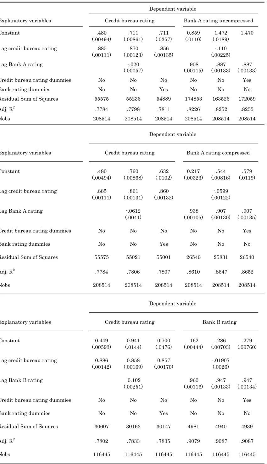
In each of the three parts of Table5 we show the results for six regressions, using data on borrowers in Bank A (employing both compressed and uncom-pressed Bank B ratings) and borrowers in Bank B. Of the six regressions in each table, four are exact estimates of equations (17)-(20). The remaining two are variations where we have included dummy explanatory variables for the lagged credit ratings instead of a simple one-period lag, in order to allow for nonlin-earities in the impact on the dependent variable. To verify that our results are robust to variations in …rm size, we also repeat the regressions, grouping by small, medium-sized, or large …rms. (These results are presented in Appendix Tables1A C,2A C, and3A C.) In Table9, we verify the robustness of our …ndings in Table5 7 with respect to estimation method by applying ordered logit instead of OLS (additional ordered logits were performed on Bank B and by size of borrower for both banks; results available upon request). Thereby
8In the actual regressions, we expect that
1c<0because higher bank credit ratings imply
we allow the ordering of the relevant dependent rating variable to occur in a nonlinear fashion with respect to the information in the explanatory variables. By also including dummy variables in the ordered logit models, we attempt to control for the widest range of nonlinearities in the data. In Section 4.1.3, we present some further robustness tests.
Hereafter we will focus on results from the "full" regressions and refer to the subsets only when di¤erences occur. When contrasting the results in each part of Table5, we will focus on the robust t-statistic on the lag of the credit bureau rating in the regression explaining the bank rating and compare di¤erences in the RSS across regressions.
4.1.1 Hypothesis 1
When considering the results for equations (17)-(18), the overall results make clear that, with between 12,000 and 200,000 observations, even small coe¢ cients are signi…cant. For both banks, we obtain highly statistically signi…cant negative coe¢ cients for the …rst lag of the credit bureau rating in regressions with a bank credit rating as the dependent variable (Table5, column 5).9 This result is robust to transformations of the rating scale (part 1 to part 2 of Table 5), to variation in …rm size and independent of the estimation method (Table 5
vs. Table9).10 We also ran regressions where we replace the lagged dependent
variable by lagged dummy variables. However, doing so invariably worsened the …t of the regression (results are not displayed here but are available upon request).
The smallest coe¢ cients on the lag of the credit bureau ratings are in the order of .01-0.2 in the OLS regressions for Bank B and in the range 0.05-0.10 for Bank A. Even taking into account the di¤erent scales that the two banks employ, this suggests that credit bureau ratings are more informative for pre-dicting ratings in Bank A than in Bank B. In columns (4)-(6) of Table5, we see that Bank A credit ratings remain relatively forecastable even when they are compressed, although not as much as the uncompressed ratings. Typically, adding lagged credit bureau ratings to the regression (column 5) reduces the RSS by more than when a lag of Bank A’s rating is added to a regression on the credit bureau rating (column 2). The only exception is made up by the subset
9Coe¢ cients are negative because credit bureau ratings follow an inverted scale relative to bank credit ratings.
1 0The …rm size regressions are presented in the Appendix Tables 1 3. The Appen-dix is available at www.riksbank.com/research/roszbach and www.phil.frb.org/research-and-data/economists/nakamura/.
of large borrowers. For those borrowers, Bank A’s ratings are, on the margin, more informative in predicting credit bureau ratings than credit bureau ratings are reversely.
The general observation that Bank A ratings are less informative is con…rmed by the results in Table7. There, we summarize the additional explanatory power of lagged credit bureau ratings when these are added to a regression of bank credit ratings on their own one-quarter lag. For example, the number 2.67 in Table 7 equals the percentage decrease in RSS when moving from column 4 to column 5 in Table 5). Depending on the size of the borrowers, credit bureau ratings explain between 2.08 and 3.01 percent of the RSS for Bank A, compared with .58 - 0.90 percent for Bank B. For Bank A, credit bureau ratings are most informative in predicting small business ratings. An inspection of the corresponding results for Bank B reinforces this picture. Adding one lag of the Bank B rating lowers the RSS of the credit bureau regression substantially more than adding the same lag of the credit bureau rating lowers Bank B’s rating RSS. This holds both for the complete sample of borrowers and in all three of the subsamples. Columns (1) and (2) of Table7 also make it clear that Bank B ratings are more informative than Bank A ratings with respect to the credit bureau ratings, as adding the former reduces the RSS by more than adding the latter does. The ordered logit regressions in columns (4)-(6) of Table9broadly con…rm the …ndings in the OLS regressions.
When reading Table 7, marginal contributions in a range between .58 and 3.01 percent may at …rst sight suggest that neither bank nor credit bureau ratings are particularly informative and that any conclusions from these ratings should be downplayed. However, bank and credit bureau ratings, both being predictors of future default risk, are constructed using a set of risk factors that is - or at least should be - close to perfectly overlapping.11 Public credit ratings
are or should be based on all publicly available information, while internal bank credit ratings are based on public information and private information. As a consequence, a regressions of any of these ratings on a lag of itself or the other rating will by construction produce only a relatively small marginal increase in the R2 or Pseudo-R2 when the the lag of the other rating is added. The
size of the marginal increase in the R2 or Pseudo-R2 can be thought of as the
contribution of private information in a regression of the bank rating and as the e¢ ciency loss of the bank rating in a regression of the credit bureau rating.
1 1See Jacobson, Lindé and Roszbach (2006) for evidence on bank ratings and Jacobson et al. (2008) for evidence on bankruptcy data.
The relative size of these two marginal e¤ects provides a means to benchmark e¢ ciency gains and losses in the collection and processing of information in the production of credit ratings.
Overall, the above …ndings constitute distinct evidence against the hypothe-sis that bank ratings are fully e¢ cient and not predicted by lagged credit bureau ratings. Moreover, the results clearly indicate that this holds all the more for bank A , and that Bank A ratings are relatively less informative.
4.1.2 Hypothesis 2
When examining the robust t-statistic on the lag of the bank rating in a re-gression of the contemporaneous credit bureau rating, we again …nd highly sig-ni…cant negative coe¢ cients in all cases. As before, this …nding is robust to variations in …rm size, to transformations of the rating scale (…rst part to the second part of Table5), to varying the estimation method (Table 5 vs. Table
9) and stable across banks (…rst two parts of Tables5 vs. the third part).12 As in Section 4.1.1 we verify that the results are robust to an exchange of the lagged bank rating by a set of lagged rating dummies. The results of this regression are shown in column (3) of Table 5, and the individual coe¢ cients on the Bank A rating dummies are displayed in Table 6. Evidently, there is nonlinear information in the Bank A ratings. Unfortunately, the coe¢ cients turn out to be non-monotonic in the rating. In other words. the improvement in the regression RSS is caused in part by the fact that the order of the ratings does not properly re‡ect the risk ranking, as measured by the credit bureau ratings. The coe¢ cients for Bank A rating grades 5 and 8 are, for example, signi…cantly greater than for the two following ratings, i.e., grades 6-7 and 9-10 respectively. The additional explanatory power of the Bank A rating dummies is thus due to rating di¤erences that do not correspond to their ordinal rank! This is strong prima facie evidence that Bank A’s ratings are not adequately capturing relative risk and that worse bank credit ratings sometimes correspond to improved credit bureau ratings. It can then hardly be expected that these bank credit ratings are strictly ordinally related to an underlying optimal measure of creditworthiness in any appropriate way. Thus our decision to compress the ratings seems justi…ed.
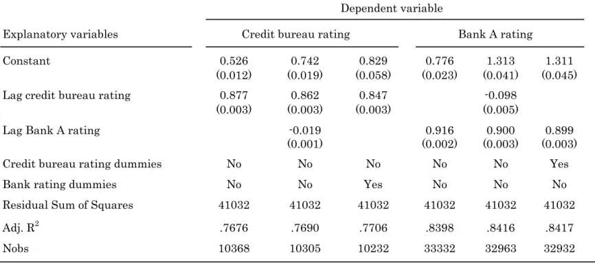
Some interesting di¤erences can be observed between the banks. For exam-ple, if we add the lagged Bank A rating in an OLS regressions of the credit bureau rating on its own lag, then the RSS drops from 55575 (column 1, Table
5) to 55236 (column 2), a reduction of less than 0.6 percent. Interestingly, when adding the credit bureau rating to a regression of the Bank A credit rating on its own lag the RSS falls to from 174853 to 163526, a decrease of over 6 percent. Thus, over the entire portfolio, the credit bureau appears to have better infor-mation than the bank since it has a proportionally bigger impact on the error! In this context, it is worthwhile to recall that we concluded in Section 2.1 that the maximum attainable decline in the RSS is 25 percent. A decrease of over 6 percent is thus a very large proportion of the change in the signal.
Above, we already argued that the uncompressed Bank A ratings su¤er from some suboptimality. The extremely large degree of forecastability of the Bank A credit ratings o¤ered additional evidence in this direction. As we mentioned earlier, columns (5)-(6) in Table5show that Bank A credit ratings are relatively well forecastable by public credit bureau ratings. By contrast, appending the lag of the credit bureau rating to a regression on the Bank B rating in Table
5 only reduces the RSS by 0.8 percent. However, adding the lagged Bank B rating reduces the RSS of the credit bureau rating regression by 1.3 percent. Bank B thus has relatively better information than the credit bureau. Ordered Logit regressions presented in the Appendix show that these …ndings are not sensitive to the estimation method one uses. Even here, Bank B appears as a relatively better rater.13
On the whole, the above …ndings o¤er strong evidence in support of the hypothesis that the banks in our sample have private information and that their internal ratings predict credit bureau ratings. We also corroborate our earlier conclusion that Bank A ratings appear less informative than Bank B ratings.
1 3The results in the ordered logit regressions resemble those in the OLS regressions. Con-sistent with our earlier …ndings, we see in Appendix Tables4A D;5A Dand6A Dthat Bank A is not as apt a rater as Bank B is. A regression of the credit bureau rating on its own lag gives a pseudo-R2of .5053, and adding the lag of the Bank A compressed rating raises the
pseudo-R2 by .0027 to .5080. By comparison, the regression of Bank A’s compressed rating
on its own lag gives a pseudo R2 of approximately .6981. Adding the lagged information
present in the bureau rating improves the …t, by .0053 to .7034. Although the contrast is not as clear as in the OLS regressions, the ordered logit regressions o¤er little evidence that Bank A’s information collection and processing are superior to that by the credit bureau. As in the OLS regressions, the same image that Bank B is a relatively better rater emerges from Tables6A D. Adding its lag increases the pseudo-R2of the regression forecasting the credit
bureau rating by .0051, from .5113 to .5164. By contrast, adding the credit bureau lag to the regression forecasting the Bank B credit rating raises it only .0036.
4.1.3 Robustness
In the theoretical model of Section 2.1, we implicitly made two assumptions about the format and updating frequency of the credit ratings. To start with, credit ratings were allowed to be continuous. Moreover, we treated the banks and the credit bureau as if they update their ratings simultaneously in each time period. The actual credit rating data we work with depart from these assumptions in two respects.
A …rst deviation from the model’s assumptions occurs because credit ratings are categorical, not continuous, variables. In moving from continuous variables to categorical variables, the bank rating may lose information, thereby making the credit bureau data more valuable. When bank credit ratings are categorical, some of the information in the public signal is not captured in the bank’s credit rating. If credit bureau ratings are continuous, the public monitor’s rating will contain information that has been lost in the aggregation. Then the public monitor’s rating may well predict the bank’s signal, even though the bank is fully aware of the public signal and "processes" it optimally. However, when both public and private monitors produce categorical ratings, we can no longer be sure what impact the loss of information due to converting continuous projections into categorical ratings will have on the mutual forecasting power of public and private ratings.
Second, our data set does not allow us to control for the exact time at which updating of information sets takes place. Hence, bank and credit bureau ratings may be staggered, without the data explicitly accounting for di¤erences in information sets between monitors. The data-providing banks update their credit ratings at least once a year, and in practice do so close to once per year on average. The credit bureau collects data from …nancial institutions, corporations, and o¢ cial resources at a higher frequency. For payments remarks, this occurs more or less daily while for other variables this typically happens at a yearly, and sometimes at monthly, quarterly, frequency. In some instances the credit bureau may thus have updated its credit rating more recently than the bank. This can create a potential for credit bureau ratings to forecast the bank ratings. At other times, banks may already have received parts of a company’s …nancial statement before it was …led. In our regression results in Table 8, this would generate an upward bias in the estimated amount of private information. To accomodate these deviations from our model assumptions, we relaxed the tests of Hypotheses 1 and 2 in Sections 4.1.1 and 4.1.2. In practice, we relaxed
the parameter restriction on the lagged dependent variable.
To address potential concerns that our …nding that bank internal credit ratings contain private information but are ine¢ cient is a result of the staggering of information sets and the coarseness of rating grades, we performed a series of robustness tests.
Staggering of information
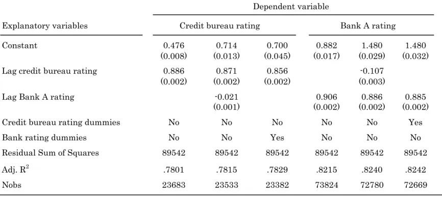
First, we repeated the regressions underlying columns 4-5 in Table5while re-stricting the data set to observations where bank ratings had just been modi…ed. Our data set does not permit us to directly observe the quarter in which the bank loan o¢ cer has collected information to review the credit ratings. What we can observe are the observations where the bank ratings have just been modi…ed. 14 Because credit ratings can only be adjusted after a loan o¢ cer has updated and …led client information, limiting us to these observations eliminates any risk that the credit bureau rating re‡ects more recent information than the bank rating. The results in Table9 show that lagged credit bureau ratings still have explanatory power for both Bank A and Bank B credit ratings. In line with our earlier …ndings, the contribution of credit bureau ratings is greater with respect to Bank A ratings than with respect to Bank B ratings. When we split up the data into small, medium-sized, and large businesses, the same pattern emerges as before: The predictive power of external ratings is manifest in the case of small businesses and least distinct with respect to larger businesses. For Bank B we cannot draw any conclusion for small businesses because of the sample size.
As a second robustness test, we replicated the regressions underlying columns 1-2 in Table5 using only observations where the credit bureau rating had just been altered. Again we …nd that restricting the data set does not bring about any changes in the results. Bank credit ratings still have predicitive power with respect to credit bureau ratings. Table9 makes it clear that just as in Section 4.1.2 Bank B ratings are better predictors of future credit ratings than Bank A ratings are. Consistent with earlier results, Bank B appears to have a slight advantage in rating larger companies.
Overall, these robustness checks demonstrate that the staggering of
infor-1 4We follow the approach of Bils, Klenow, and Malin (2009), who study staggered prices on the assumption that menu costs prevent observed prices from equaling shadow prices. They use the observations when prices change to infer underlying shadow price movements. Because most bank clients are reviewed once a year, we use four-quarter lags for the right-hand side variables in these regressions.
mation updating by the credit bureau and banks in our data, although it may occur, does not a¤ect our conclusion that our banks’internal credit ratings do contain private information, consistent with theory, but are ine¢ cient measures of creditworthiness.
Coarseness of the rating scale
As a last robustness test, we investigate whether using discrete instead of con-tinuous credit bureau ratings alters the explanatory power that we attribute to lagged bank ratings. For this purpose, we exploit that the credit bureau has not only provided us with the actual credit rating but also with the near-continuous measure of creditworthiness that is underlying its credit rating. This is a nu-merical rating that runs from 0 to 100 (from 0.5 to 1 and then by units up to 99). We take logarithms of these numerical ratings, and we re-run the regressions of columns 1 2 in Table 5 using the continuous measure of creditworthiness as a dependent variable and its lag plus the lagged discrete bank rating data as explanatory variables. In Table9, we see that bank credit ratings continue to have predictive power for credit bureau ratings, even when the latter are contin-uous. We take this as strong evidence that banks do have private information not embedded in the credit bureau ratings.
Unfortunately, we do not have similar continuous signals for the banks. Thus, the loss of information in the bank ratings could imply either that in-formation is being lost due to the discreteness of the ratings or that the banks are not e¢ ciently impounding their private information into the public infor-mation.
4.2
Survival time regressions
In the previous section, we found that bank ratings, which contain both public and private information, are only partially able to forecast credit bureau ratings that are produced using publicly available information. Vice versa, we showed that, somewhat surprisingly, credit bureau ratings are able to partially forecast internal bank credit ratings. From a research perspective, an intuitively at-tractive conclusion to be drawn from these results would be that credit bureau ratings are of higher quality than one would expect from theory, whereas bank ratings are less so. If this were the case, then we should at least expect credit bureau ratings to also be better predictors of credit bureau defaults, i.e., bank-ruptcies, than bank ratings are. Since credit bureau ratings are constructed
to predict bankruptcy, whereas bank ratings are designed to predict defaults in loan portfolios, any other …nding would cast doubt on our conclusions in Section 4.1
To verify if the above proposition holds, we therefore perform an additional test on the data and compare the explanatory power of bank credit ratings and credit bureau ratings in a duration model setting. We implement the test by estimating the following Cox proportional hazards model:
log hi(t) = (t) + xit+"it (21)
or equivalently
hi(t) =h0(t)exp( (t) + xit+"it) (22)
for a number of competing speci…cations. Here,hi(t)is the hazard rate of …rmi
at timet, (t) =log h0(t), andxcontains all time-varying covariates. The Cox model leaves the baseline hazard function unspeci…ed, thereby making relative hazard ratios both proportional to each other and independent of time other than through values of the covariates.
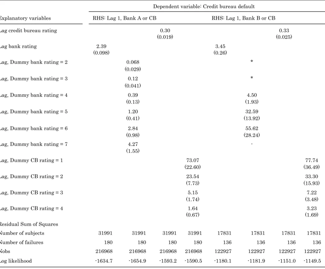
We run three sets of regressions to verify the above assertion. In the …rst group of regressions, displayed in Table 10, the main variable of interest is a …rms’hazard rate, or instantaneous risk ofbankruptcy at timetconditional on survival to that time. First, we let xit = rc;t 1 to compute the explanatory power of lagged credit bureau ratings for borrowers in both Bank A and Bank B (Table10, columns3;7). Next, we takexit=rb;t 1., whereb= 1;2(columns
1, 5). In column 2 and 4 of these tables, we present results from regressions where we let xit= h DU M_rb;t1 1; DU M_rb;t2 1::::; DU M_rGb;t 11i (23) and xit= DU M_r1c;t 1; DU M_rc;t2 1::::; DU M_rGc;t 11 (24) whereG is the number of grades in a rating system, and DU M_rgb;t 1 = 1 if rb;tg 1=gand zero otherwise.
The log likelihood values in columns 1 and 3 of Table10show that the lagged credit bureau rating is better at explaining bankruptcy hazard rates than the lagged Bank A rating is. This …nding is robust to exchanging the lagged rating
for a set of lagged rating dummies. The table also shows that the same results are obtained when using Bank B ratings instead. The Appendix (Table A7) contains output from an additional robustness test, where we repeated the above regressions using a second lag instead of the …rst lag. This does not change the results qualitatively. As one would expect, the coe¢ cients on the lagged rating dummies are monotonically increasing in risk for both the credit bureau and bank ratings. This re‡ects the fact that higher bank ratings and lower credit bureau ratings should be stronger indicators of future defaults. Hence, hazard rates should rise (fall) as bank (credit bureau) ratings become higher (lower).
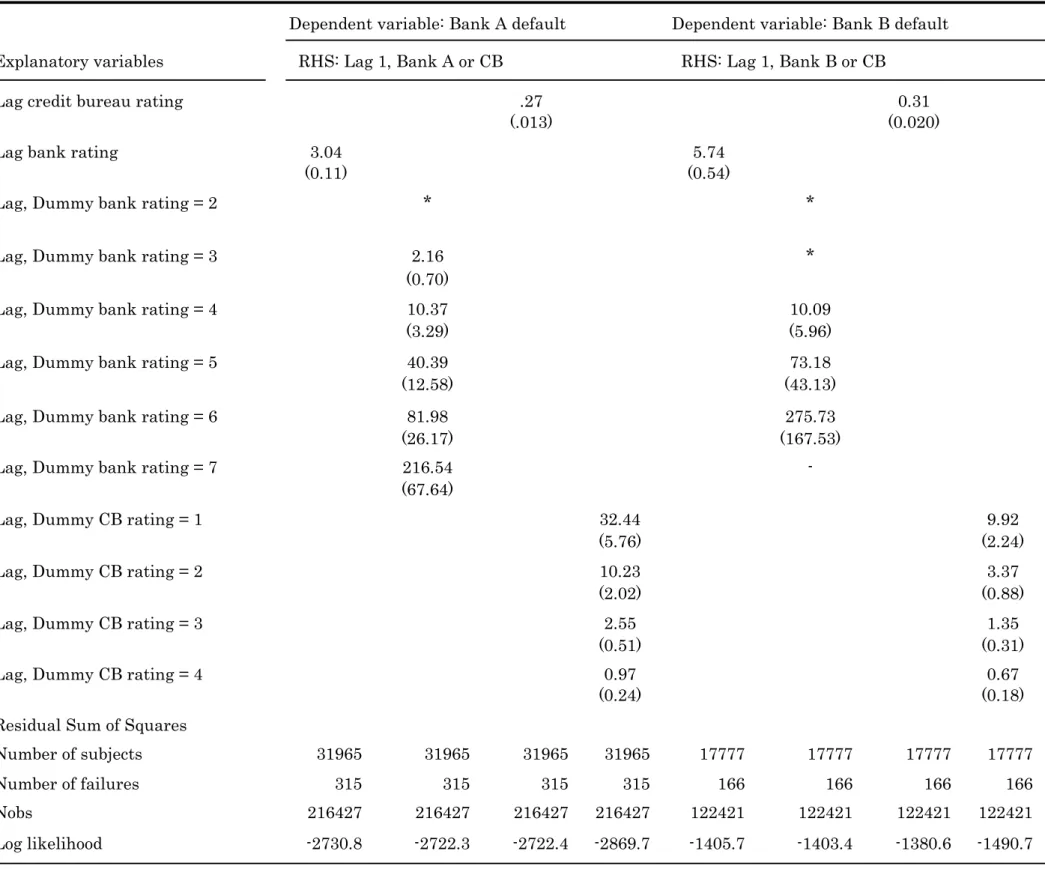
Next, in Table11, we present the results from a similar set of Cox regressions where the dependent variable is the instantaneous risk of a default in a bank at timet, conditional on survival to that time. A similar comparison between columns 1 and 3 makes it clear that for both Bank A and Bank B lagged credit bureau ratings are better at explaining bank default hazards than bank ratings are themselves. In the Appendix (Table A8) we again …nd these results are robust to exchanging the …rst lag by the second lags of the explanatory ratings. However, when we replace the lagged variables by a set of dummy variables, the credit bureau ratings lose their edge. This reversal may be indicative of the fact that the rating grades used by both banks are highly nonlinear. Thus when using a parsimonious model that is linear in its explanatory variable, thebank
ratings have less explanatory power.
The results in Tables10and11also illustrate how the nonlinearities in both bank and credit bureau ratings come into play in our analysis. Columns1and
3of Table 10show that if one imposes the restriction of equal marginal e¤ects of rating grade changes on the default hazard, then Bank A rating adjustments have a substantially greater e¤ect on the bankruptcy hazard than credit bureau ratings do. This would suggest that Bank A ratings are more informative than credit bureau ratings. However, when once the equality constraint is relaxed, this relationship reverses and adjustments of credit bureau ratings are found to have the greater impact on the hazard rate (columns2and4). This reversal is caused by the condition that default risk is very small for a nontrivial number of corporations. Deteriorations of these companies’ rating thus lead to a very large increase in the hazard rate. By imposing that each rating change must have an equally sized e¤ect on the hazard rate, the importance of such ratings changes is restricted. This loss of information is greater when using credit bureau ratings than bank ratings, most likely because the former are less persistent. A similar reversal occurs when using Bank B ratings. However, consistent with
our previous …nding that Bank B ratings are relatively more informative, the di¤erential between the dummy coe¢ cients (column6 and 8) is much smaller than for Bank A.
In Table11, we observe a comparable e¤ect of parameter restrictions when explaining loan default hazards. In a restricted Cox regression model, credit bureau ratings appear more informative, but once the equality constraint is re-laxed, the e¤ect of bank rating changes dominates that of credit bureau changes. Again consistent with our previous …ndings, the marginal increase of the loan default hazard due to a credit bureau rating adjustment is greater for Bank A than for Bank B.
In Table 12, we present the log likelihoods of the regressions that include the credit bureau rating alone, the bank ratings alone, and both credit bureau ratings and the bank ratings together. We have marked the signi…cance of the likelihood ratio tests for the credit bureau rating for exclusion of the bank rating, and vice versa. For example, the log likelihood of the model with the credit bureau rating alone in the regression using credit bureau default for all Bank A borrowers is -1593.2. As the regression that uses both the credit bureau rating and the Bank A rating has a log likelihood of -1555.2, twice the log likelihood ratio is 76.0, making the Bank A rating very signi…cant in a chi-square test with one degree of freedom. As can be seen, neither the bank ratings nor the credit bureau ratings are on their own su¢ cient statistics of default. This is true for both Bank A and Bank B and for both de…nitions of default; it also holds when we lag both ratings an additional period. In particular, this provides striking evidence that the credit bureau rating adds information to the bank rating, even though the bank loan o¢ cers have ready access to the credit bureau ratings when they make their ratings.
In the Appendix Tables A-15 to A-17, we provide additional results on the log likelihoods and exclusion tests for subsets of small, medium, and large borrowers. An interesting conclusion from those tables is that the credit bureau ratings do notably better than bank ratings for small borrowers, while the reverse tends to be true for the large borrowers.
5
Simulations
For both banks that we study, we have found that the credit bureau ratings forecast bank credit ratings. A direct implication of this is that a bank’s ratings
alone are not the best possible measure of a loan portfolio’s underlying over-all creditworthiness. There are two reasons, not mutuover-ally exclusive, why this could be happening. One possibility is that the bank’s credit ratings do not impound the credit bureau’s data optimally. The bank’s loan o¢ cers may, for example, overvalue their private information vis-à-vis the credit bureau’s rating, internal scoring models may be inadequate, or certain public information may be disregarded. Another possibility is that the rating process itself, for exam-ple through the requirement that ratings be categorical or because of staggered updating of borrower information, reduces information embedded in the bank ratings or limits its accuracy.
The …rst of these two causes is relatively hard to evaluate with the informa-tion we have available. In Secinforma-tion 4.1.3, we showed that staggered updating, although it possibly occurs, does not in‡uence our results; we also o¤ered ev-idence that the discretization of credit bureau ratings or coarsening of their rating grades does not alter our conclusion that both banks have some private information.
In this section, we attempt to obtain some more general insights into the e¤ects of discretizing credit ratings on their relative informativeness. To do so, we simulate data for the model in Section 2.1 and estimate regressions both with and without discretization of initially continuous credit ratings.
For the simulations, we generate 1,000 data series from a random walk process, each over 20 periods, which we think of as being quarters. In each period, the random walk processes, which all start at time zero, receive a stan-dard normal shock. The monitors receive signals that include noise: the random walk plus a normal temporary noise. As in the model, there are two sources of information: the public signal and the bank’ private signal. The underly-ing creditworthiness of each borrower has a disturbance term that is standard normal.
The credit bureau’s signal has a relative precision of .1. The bank’s private signal has a precision of .4, but to this is added the credit bureau’s signal Once combined with the credit bureau’s signal, the bank’s signal has a precision of .5 (an idiosyncratic variance of 2). To limit the problems associated with the long run increasing variance of the random walk, we focus on one time period, namely period 20. In the 20th period (5 years), the standard deviation of ratings is 4.4 for the bank and 4.2 for the credit bureau. The theoretical standard deviation of creditworthiness is 20.5 = 4.472, while the actual standard deviation in the sample is 4.4702. The theoretical four-quarter-ahead expected forecast variance
is 4.
As preliminary evidence on the e¤ect that coarsening of the data has, we measure the contemporaneous correlations between our simulated ratings. Note that the correlations between the credit ratings of the credit bureau and the credit ratings of banks are much lower than in the simulation. Table13shows the quarterly correlations ranging from 0.29 to 0.57, which is substantially lower than the correlations in the simulated data (not reported). This variation over time may in fact explain some of the anomalies in the data and the concomitant results with respect to Bank A. Bank B’s correlations with the credit bureau appear fairly consistent over time. Bank A’s correlations, however, vary con-siderably and appear in general to drift downward except for an abrupt rise in 1999 Q2, followed by a resumption of the downward drift. It is also worth noting that the correlations are systematically lower for original Bank A ratings than when these are coarsened to 7 grades. The extra information in the ratings does not appear to be correlated with information in the credit bureau ratings. Additional analysis (not presented here) shows that the correlations are more or less unchanged when we use rank correlations instead.
In the Appendix, we present the results from an OLS regression on simulated data where credit ratings are continuous and rating updating takes place without staggering.15 In a regression of the credit bureau rating on one lag of itself, the
lag of the bank rating is highly signi…cant when added. Moreover, when added to a regression of the simulated bank credit rating on a lag of itself, the lag credit bureau rating is not signi…cant. The contemporaneous correlation between the bank and credit bureau rating in the simulated data is .9764.
When we break up the continuous signals into six evenly spaced categories and re-run the above set of regressions, the coe¢ cient on the lagged credit bu-reau rating becomes both signi…cant and quantitatively more important. In addition, the RSS of forecasts of the bank’s credit ratings drop substantially when the lagged credit bureau rating is included. Interestingly, the contempo-raneous correlation falls only slightly, to .9436. When we simulate data that are both staggered and aggregated into six intervals, the outcomes reveal that there is no monotonic relationship between the noisiness of the ratings and the size of the coe¢ cient for the lagged bank rating. The simulations do suggest that the RSS falls monotonically as ratings become more noisy. Similar results are obtained when ordered logit models are estimated instead of OLS.