Open Access Dissertations Theses and Dissertations
12-2016
Differentially private data publishing for data
analysis
Dong Su
Purdue University
Follow this and additional works at:https://docs.lib.purdue.edu/open_access_dissertations Part of theComputer Sciences Commons
This document has been made available through Purdue e-Pubs, a service of the Purdue University Libraries. Please contact [email protected] for additional information.
Recommended Citation
Su, Dong, "Differentially private data publishing for data analysis" (2016).Open Access Dissertations. 1005.
PURDUE UNIVERSITY GRADUATE SCHOOL Thesis/Dissertation Acceptance
This is to certify that the thesis/dissertation prepared By
Entitled
For the degree of
Is approved by the final examining committee:
To the best of my knowledge and as understood by the student in the Thesis/Dissertation Agreement, Publication Delay, and Certification Disclaimer (Graduate School Form 32), this thesis/dissertation adheres to the provisions of Purdue University’s “Policy of Integrity in Research” and the use of copyright material.
Approved by Major Professor(s):
Approved by:
Head of the Departmental Graduate Program Date
Dong Su
Differentially Private Data Publishing for Data Analysis
Doctor of Philosophy Ninghui Li Chair Elisa Bertino Christopher W. Clifton Jennifer Neville Ninghui Li
FOR DATA ANALYSIS
A Dissertation Submitted to the Faculty
of
Purdue University by
Dong Su
In Partial Fulfillment of the Requirements for the Degree
of
Doctor of Philosophy
December 2016 Purdue University West Lafayette, Indiana
ACKNOWLEDGMENTS
I would like to express my deepest gratitude and appreciation to my advisor, Dr. Ninghui Li, for his guidance and supervision and the many opportunies that he has af-forded me. He is always available, friendly, and helpful with amazing insights. I am so fortunate to have the opportunity to work with him in my graduate study. Without his help and support, this dissertation would not have been possible. I will be forever indebted to him for what he has given to me.
My appreciation also goes to my prelim exam committee and final exam committee: Dr. Elisa Bertino, Dr. Christopher W. Clifton, Dr. Dan Goldwasser and Dr. Jennifer Neville for their helpful advice and suggestions on my dissertation.
I would also like to express my gratitude to my research collaborators, Dr. Jianneng Cao, Dr. Min Lyu, Dr. Elisa Bertino and Dr. Hongxia Jin. In the past years, I greatly benefited from their constructive suggestions and effective discussions.
I am fortunate to be in Purdue with an amazing group of fellow students. I am grateful to them for their friendship and support throughout.
Last but not least, my hearfelt appreciation goes to my family. I can always feel their love, bless and support.
TABLE OF CONTENTS
Page
LIST OF TABLES . . . vi
LIST OF FIGURES . . . viii
ABSTRACT . . . xi
1 INTRODUCTION . . . 1
2 PRELIMINARIES AND RELATED WORKS . . . 4
2.1 The Definition ofǫ-DP . . . 4
2.1.1 Bounded DP or Unbounded DP . . . 5
2.2 Properties ofǫ-DP . . . 5
2.2.1 Post-processing and Sequential Composition . . . 6
2.2.2 Parallel Composition and Convexity . . . 8
2.3 The Laplace Mechanism . . . 11
2.3.1 The Scalar Case . . . 11
2.3.2 The Vector Case . . . 14
2.4 The Exponential Mechanism . . . 16
2.4.1 The General Case of the Exponential Mechanism . . . 16
2.4.2 The Monotonic Case of the Exponential Mechanism . . . 17
2.5 Settings to Apply DP. . . 19
2.6 Differentially Private Data Analysis . . . 21
2.6.1 Example Optimization Problems . . . 23
2.6.2 Objective Perturbation . . . 26
2.6.3 Make an Existing Algorithm Private . . . 30
2.6.4 Iterative Local Search via EM . . . 36
2.6.5 Histograms Optimized for Optimization . . . 40
Page
3.1 Introduction . . . 43
3.2 PrivPfC Framework . . . 45
3.2.1 The Quality Function . . . 46
3.2.2 Sensitivity in the Binary Classification Case . . . 48
3.2.3 Sensitivity of Grid Quality in the Multiclass Classification Case 54 3.2.4 Candidate Grids Enumeration . . . 57
3.2.5 Putting Things Together for PrivPfC . . . 59
3.3 Experiment. . . 59
3.3.1 Experimental Settings . . . 59
3.3.2 Comparison with Existing Solutions . . . 68
3.3.3 Varying Parameters in PrivPfC . . . 70
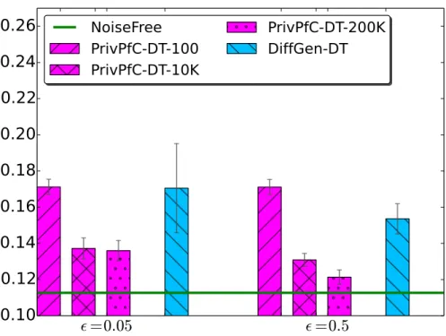
3.3.4 Analyses of Sources of Errors . . . 71
3.3.5 Scalability over Dimensions and Runtime . . . 73
4 DIFFERENTIALLY PRIVATEk-MEANS CLUSTERING . . . 75
4.1 Introduction . . . 75
4.2 Differentially Private Lloyd Algorithm and Its Improvements . . . 78
4.2.1 DPLloyd . . . 79
4.3 Other Approaches . . . 86
4.3.1 PGkM . . . 86
4.3.2 GkM . . . 88
4.4 Using a Private Synopsis . . . 90
4.4.1 MkM . . . 91
4.4.2 UGkM . . . 91
4.4.3 EUGkM . . . 92
4.5 The Hybrid Approach . . . 93
4.5.1 Error Study of EUGkM . . . 95
4.5.2 Hybrid Approach . . . 97
Page
4.6.1 Evaluation Methodology. . . 101
4.6.2 Experimental Results. . . 105
4.6.3 Performance of the Hybrid Approach . . . 107
4.6.4 The Analysis of the GkM Approach . . . 108
4.6.5 The Analysis of the PGkM Approach . . . 110
4.6.6 The Analysis of the EUGkM, UGkM and MkM Approaches . . 111
4.6.7 Estimating the Number of Clusters. . . 112
5 UNDERSTANDING THE SPARSE VECTOR TECHNIQUE . . . 118
5.1 Introduction . . . 118
5.2 Variants of SVT . . . 121
5.2.1 Privacy Proof for Proposed SVT . . . 129
5.2.2 Privacy Properties of Other Variants . . . 133
5.2.3 Error in Privacy Analysis of GPTT . . . 135
5.2.4 Other Variants . . . 137
5.3 Optimizing SVT . . . 138
5.3.1 A Generalized SVT Algorithm . . . 138
5.3.2 Optimizing Privacy Budget Allocation . . . 140
5.3.3 SVT for Monotonic Queries . . . 141
5.4 SVT versus EM . . . 143 5.5 Evaluation . . . 145 5.6 Related Work . . . 161 6 SUMMARY . . . 162 REFERENCES . . . 163 VITA. . . 169
LIST OF TABLES
Table Page
3.1 Dataset characteristics . . . 66
3.2 Summary of differentially private classification methods . . . 67
4.1 Descriptions of datasets. . . 99
4.2 Summary of differentially privatek-means methods . . . 100
4.3 Likelihood of the Top-4 Selected k values based on RT-validity over S1 and Gowalla datasets. . . 115
4.4 Likelihood of the Top-4 Selectedkvalues based on RT-validity over the TIGER and Image datasets. . . 116
4.5 Likelihood of the Top-4 Selectedkvalues based on RT-validity over the Adult-num and Lifesci datasets. . . 117
5.1 Dataset characteristics . . . 145
5.2 Summary of algorithms . . . 146
5.3 Comparison of SVT-DPBook, SVT-S, SVT-ReTr and EM on selecting top-c queries in terms of SER whenǫ= 0.1on datasets BMS-POS and Kosarak. For each row, the best SER value in the non-interactive setting is marked by italics and the best SER value in the interactive setting is marked by boldface. Each cell gives the average value of SER with standard deviation. . . 157
5.4 Comparison of SVT-DPBook, SVT-S, SVT-ReTr and EM on selecting top-c queries in terms of SER when ǫ = 0.1on datasets AOL and Zipf. For each row, the best SER value in the non-interactive setting is marked by italics and the best SER value in the interactive setting is marked by boldface. Each cell gives the average value of SER with standard deviation. . . 158
5.5 Comparison of SVT-DPBook, SVT-S, SVT-ReTr and EM on selecting top-c queries in terms of SER whenǫ= 0.5on datasets BMS-POS and Kosarak. For each row, the best SER value in the non-interactive setting is marked by italics and the best SER value in the interactive setting is marked by boldface. Each cell gives the average value of SER with standard deviation. . . 159
5.6 Comparison of SVT-DPBook, SVT-S, SVT-ReTr and EM on selecting top-c
queries in terms of SER when ǫ = 0.5on datasets AOL and Zipf. For each
row, the best SER value in the non-interactive setting is marked by italics and the best SER value in the interactive setting is marked by boldface. Each cell
LIST OF FIGURES
Figure Page
2.1 Differential privacy via Laplace noise. . . 12
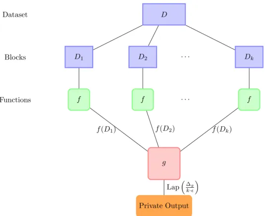
2.2 An illustration of the sample and aggregate framework. . . 35
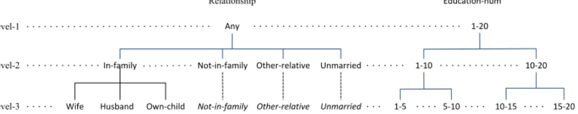
3.1 Taxonomy hierarchies of Relationship attribute and Education-num attribute. 45
3.2 Illustration of the sensitivity of grid quality (Eq. 3.3). . . 49
3.3 Correlation between grid quality (Eq 3.1) and its approximation (Eq 3.8).
Av-erage Pearson correlation coefficient is 0.936 with standard deviation 0.026. 55
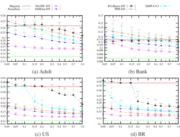
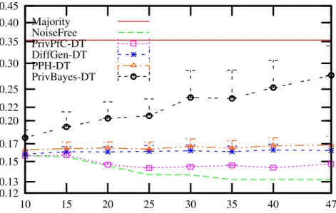
3.4 Comparison of PrivPfC, DiffGen, PrivBayes, PPH and DiffPC-4.5 by decision
tree classification. x-axis: privacy budgetǫin log-scale. y-axis:
misclassifica-tion rate in log-scale.. . . 60
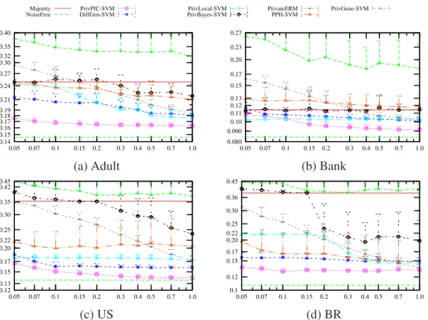
3.5 Comparison of PrivPfC, DiffGen, PrivBayes, PPH, PrivGene and PrivateERM
by SVM classification. x-axis: privacy budgetǫin log-scale. y-axis:
misclas-sification rate in log-scale. . . 61
3.6 Comparison of PrivPfC, DiffGen, PrivBayes, PPH and FunctionalMechanism
by logistic regression classification. x-axis: privacy budgetǫ in log-scale.
y-axis: misclassification rate in log-scale. . . 62
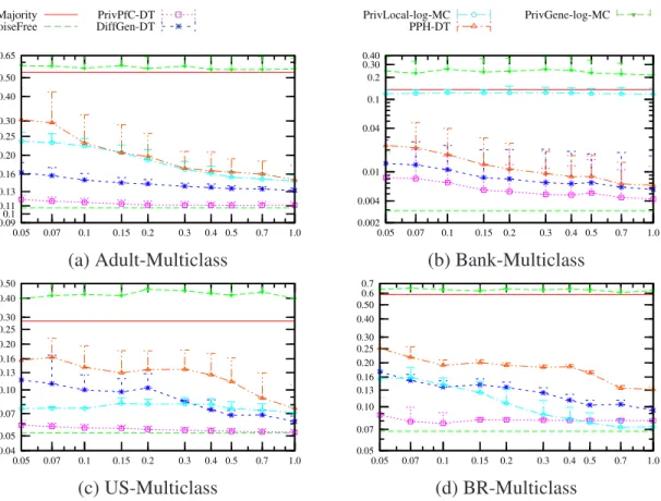
3.7 Comparison of PrivPfC, DiffGen, PPH, PrivLocal and PrivGene by
deci-sion tree classification and logistic regresdeci-sion classification on the multiclass
datasets. y-axis: misclassification rate in log-scale. . . 68
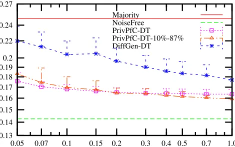
3.8 Varying the maximum pool size Ω on PrivPfC by decision tree classification
on the BR dataset. y-axis: misclassification rate. . . 70
3.9 Comparison of two different privacy budget allocations on PrivPfC by decision
tree classification on the Adult dataset. y-axis: misclassification rate in
log-scale. . . 71
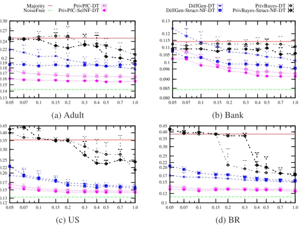
3.10 Analyses of PrivPfC, DiffGen and PrivBayes by decision tree classification.
x-axis: privacy budgetǫin log-scale. y-axis: misclassification rate in log-scale. 72
3.11 Comparison of PrivPfC, DiffGen, PrivBayes and PPH by varying dimensions
(decision tree classification). ǫ= 0.5. x-axis: dimensions. y-axis:
Figure Page 3.12 Runtime comparison of PrivPfC, DiffGen, PPH and PrivBayes on decision tree
classification. x-axis: privacy budget. y-axis: runtime in seconds. . . 74
4.1 The comparison of DPLloyd-Impr, PGkM, GkM, EUGkM, UGkM and MkM by varying the privacy budgetǫ. x-axis: privacy budgetǫin log-scale. y-axis: NICV in log-scale. . . 101
4.2 The close-up view of the comparison of DPLloyd-Impr, DPLloyd, EUGkM, and UGkM by varying the privacy budget ǫ. x-axis: privacy budgetǫ in log-scale. y-axis: NICV in log-log-scale. . . 102
4.3 The heatmap by varyingkanddon the Synthe datasets withǫ= 1.0. . . 103
4.4 The heatmap by varyingkanddon the Synthe-PT datasets. ǫ = 1.0. Varying theθvalue in EUGkM. . . 107
4.5 The comparison of the Hybrid approach with EUGkM and DPLloyd-Impr. x-axis: privacy budgetǫin log-scale. y-axis: NICV in log-scale. . . 109
4.6 The analysis of the GkM Approach. x-axis: block size exponent in log-scale, y-axis: NICV in log-scale. . . 110
4.7 The comparison of the convergence rate of the genetic algorithm based k -means and Lloyd algorithm. x-axis: number of iterations in log-scale, y-axis: NICV in log-scale. . . 112
4.8 Comparing running time between DPLloyd and EUGkM,ǫ = 0.1. . . 114
5.1 An instantiation of the SVT proposed in this chapter . . . 121
5.2 SVT in Dwork and Roth 2014 [76] . . . 122
5.3 SVT in Roth’s 2011 Lecture Notes [73] . . . 123
5.4 SVT in Lee and Clifton 2014 [69] . . . 124
5.5 SVT in Stoddard et al. 2014 [70]. . . 125
5.6 SVT in Chen et al. 2015 [71] . . . 126
5.7 Differences among Algorithms 17-22. . . 127
5.8 The distribution of 300 highest scores from experiment datasets. . . 146
5.9 Comparison of interactive approaches: SVT-DPBook and SVT-S with different budget allocation,ǫ= 0.1, BMS-POS and Kosarak datasets. x-axis: top-c . 149 5.10 Comparison of interactive approaches: SVT-DPBook and SVT-S with different budget allocation,ǫ= 0.1, AOL and Zipf datasets. x-axis: top-c . . . 150
Figure Page 5.11 Comparison of interactive approaches: SVT-DPBook and SVT-S with different
budget allocation,ǫ= 0.5, BMS-POS and Kosarak datasets. x-axis: top-c . 151
5.12 Comparison of interactive approaches: SVT-DPBook and SVT-S with different
budget allocation,ǫ= 0.5, AOL and Zipf datasets. x-axis: top-c . . . 152
5.13 Comparison of non-interactive approaches: EM and SVT-ReTr with different
thresholds,ǫ= 0.1, BMS-POS and Kosarak datasets. x-axis: top-c . . . 153
5.14 Comparison of non-interactive approaches: EM and SVT-ReTr with different
thresholds,ǫ= 0.1, AOL and Zipf datasets. x-axis: top-c . . . 154
5.15 Comparison of non-interactive approaches: EM and SVT-ReTr with different
thresholds,ǫ= 0.5, BMS-POS and Kosarak datasets. x-axis: top-c . . . 155
5.16 Comparison of non-interactive approaches: EM and SVT-ReTr with different
ABSTRACT
Su, Dong PhD, Purdue University, December 2016. Differentially Private Data Publishing for Data Analysis. Major Professor: Ninghui Li.
In the information age, vast amounts of sensitive personal information are collected by companies, institutions and governments. A key technological challenge is how to design mechanisms for effectively extracting knowledge from data while preserving the privacy of the individuals involved. In this dissertation, we address this challenge from the perspec-tive of differentially private data publishing. Firstly, we propose PrivPfC, a differentially private method for releasing data for classification. The key idea underlying PrivPfC is to privately select, in a single step, a grid, which partitions the data domain into a num-ber of cells. This selection is done using the exponential mechanism with a novel quality function, which maximizes the expected number of correctly classified records by a his-togram classifier. PrivPfC supports both the binary classification as well as the multiclass
classification. Secondly, we study the problem of differentially privatek-means clustering.
We develop techniques to analyze the empirical error behaviors of the existing interactive and non-interactive approaches. Based on the analysis, we propose an improvement of the DPLloyd algorithm which is a differentially private version of the Lloyd algorithm and pro-pose a non-interactive approach EUGkM which publishes a differentially private synopsis
fork-means clustering. We also propose ahybridapproach that combines the advantages
of the improved version of DPLloyd and EUGkM. Finally, we investigate the sparse vec-tor technique (SVT) which is a fundamental technique for satisfying differential privacy in answering a sequence of queries. We propose a new version of SVT that provides better utility by introducing an effective technique to improve the performance of SVT in the in-teractive setting. We also show that in the non-inin-teractive setting (but not the inin-teractive setting), usage of SVT can be replaced by the exponential mechanism.
1. INTRODUCTION
Data collected by organizations and agencies are a key resource in today’s information age. The use of sophisticated data mining techniques makes it possible to extract relevant knowledge that can then be used for a variety of purposes, such as research, product de-velopment and public policy making. However, the disclosure and exploration of those data pose serious threats to individual privacy. Examples include the identification of the medical record of the governor of Massachusetts from the GIC data [1]; the identification of the search history of an AOL user from the AOL query log data [2]; the identification of Netflix subscribers from the Netflix Prize dataset [3] and the identification of participants from the published aggregated DNA statistics in the Genome-Wide Association Studies (GWAS) [4].
In this dissertation, we consider the problem of private data publication. In this setting, a trusted data curator gathers sensitive information from a large number of respondents, create a microdataset where each tuple corresponds to one entity, such an individual, a household or an organization, and release the sanitized synopsis to the public.
In recent years, differential privacy [5, 6] has emerged as thede factostandard privacy
notion for private data analysis because it offers a rigorous guarantee of privacy regard-less of the adversary’s prior knowledge. Differential privacy requires that the output of a data analysis mechanism be approximately identical, even if any single tuple in the input
database is arbitrarily added or removed. Differential privacy is parameterized by ǫ, the
upper bound of the ratio of the probabilities on getting the same output on the above two
database differing in a single tuple. ǫmeasures the privacy risk. The smaller the ǫis, the
harder for the adversary to infer the existence of the target tuple in the database.
We aim at developing practical techniques to data analysis under differential privacy. There are two broad approaches for differentially private data analysis. The interactive approach aims at developing customized differentially private algorithms for various data
analysis tasks. The non-interactive approach aims at developing differentially private algo-rithms that can output a synopsis of the input dataset, which can then be used to support various data mining tasks. Most of existing works focus on developing interactive ap-proaches [7–12]. However, the interactive approach is far from being practical since the limited privacy budget has to be shared by all queries issued to the database. On the other hand, non-interactive approaches are free from this limitation. However, very few prac-tical and accurate non-interactive private data publishing algorithms have been proposed. Therefore, in this dissertation, we attempt to provide solutions for differentially private data analysis by proposing new non-interactive algorithms and combining the advantages of two approaches.
We begin in Chapter 3 by introducing PrivPfC, a differentially private method for re-leasing data for classification. Several state-of-the-art methods follow the structure of ex-isting classification algorithms and are all iterative, which is suboptimal due to the locally optimal choices and division of the privacy budget among many sequentially composed steps. We propose PrivPfC, a new differentially private method for releasing data for clas-sification. The key idea underlying PrivPfC is to privately select, in a single step, a grid, which partitions the data domain into a number of cells. This selection is done using the ex-ponential mechanism with a novel quality function, which maximizes the expected number of correctly classified records by a histogram classifier. PrivPfC supports both the binary classification as well as the multiclass classification. Through extensive experiments on real datasets, we demonstrate PrivPfC’s superiority over the state-of-the-art methods.
In Chapter 4, we focus on differentially private k-means clustering. Several
state-of-the-art methods follow the single-workload approach which adapts an existing machine
learning algorithm by making each step private. However, most of them do not have sat-isfactory empirical performance. In this work, we develop techniques to analyze the em-pirical error behaviors of one of the state-of-the-art single-workload approaches, DPLloyd, which is a differentially private version of the Lloyd algorithm. Based on the analysis,
we propose an improvement of DPLloyd. We also propose a new algorithm fork-means
of the input dataset. After analyzing the empirical error behaviors of EUGkM, we further
propose a hybrid approach that combines our DPLloyd improvement and EUGkM.
Re-sults from extensive and systematic experiments support our analysis and demonstrate the effectiveness of the DPLloyd improvement, EUGkM and the hybrid approach.
In Chapter 5, we focus on the sparse vector technique. The Sparse Vector Technique (SVT) is a fundamental technique for satisfying differential privacy and has the unique quality that one can output some query answers without apparently paying any privacy cost. SVT has been used in both the interactive setting, where one tries to answer a se-quence of queries that are not known ahead of the time, and in the non-interactive setting, where all queries are known. Because of the potential savings on privacy budget, many variants for SVT have been proposed and employed in privacy-preserving data mining and publishing. However, most variants of SVT are actually not private. In this dissertation, we analyze these errors and identify the misunderstandings that likely contribute to them. We also propose a new version of SVT that provides better utility, and introduce an effec-tive technique to improve the performance of SVT. These enhancements can be applied to improve utility in the interactive setting. In the non-interactive setting (but not the interac-tive setting), usage of SVT can be replaced by the Exponential Mechanism (EM); we have conducted analytical and experimental comparisons to demonstrate that EM outperforms SVT.
Our overall contribution can be summarized as follows. On differentially private classi-fication, we propose a non-interactive approach for publishing projected histograms, which results in lower classification error when compared with the current state-of-the-art
meth-ods. On differentially private k-means clustering, we propose the EUGkM method for
publishing synopsis fork-means clustering, which outperforms existing methods. We also
propose a novel hybrid approach to differentially private data analysis, which is so far the
best approach tok-means clustering. On SVT, we propose a new version of it that provides
better utility, and introduce an effective technique to improve the performance of SVT in the interactive setting. We also showed that in the non-interactive setting, usage of SVT can be replaced by the Exponential Mechanism (EM).
2. PRELIMINARIES AND RELATED WORKS
2.1 The Definition ofǫ-DP
Informally, the DP notion requires any single element in a dataset to have only a limited impact on the output. The following definition is taken from [5, 6].
Definition 2.1.1 (ǫ-Differential Privacy) An algorithm A satisfies ǫ-differential privacy (ǫ-DP), whereǫ ≥ 0, if and only if for any datasetsDandD′ thatdiffer on one element,
we have
∀T ⊆Range(A) : Pr[A(D)∈T]≤eǫPr[A(D′)∈T], (2.1)
whereRange(A)denotes the set of all possible outputs of the algorithmA.
The condition (2.1) can be equivalently stated as:
∀t ∈Range(A) : Pr[A(D) = t]
Pr[A(D′) =t] ≤e
ǫ, (2.2)
where we define 00 to be1.
More generally, ǫ-DP can be defined by requiring Eq. (2.1) to hold onD andD′ that
are neighboring. When applying DP, an important choice is the precise condition under
whichD andD′ are considered to be neighboring. Even when applying DP to relational
datasets and interpreting “differing by one element” as “differing by a single record (or tuple)”, there are still two natural choices, which lead to what are called unbounded and
bounded DP in [13]. InUnbounded DP, Dand D′ are neighboring ifD can be obtained
fromD′ by adding or removing one element. InBounded DP,D andD′ are neighboring
ifDcan be obtained fromD′ by replacing one element inD′with another element. When
using bounded DP, two datasets that have different number of elements are not considered to be neighboring; therefore, publishing the exact number of elements in the input dataset
satisfiesǫ-DP for anyǫunder bounded DP. However, doing so does not satisfyǫ-DP for any
ǫin unbounded DP.
One way to understand the intuition of DP is the following “opting-out” analogy. We
want to publishA(D), whereDconsists of data of many individuals. An individual objects
to publishingA(D)because her data is inD and she is concerned about her privacy. In
this case, we can address the individual’s privacy concern by removing her data fromD(or
replacing her data with some arbitrary value) to obtainD′and publishingA(D′). However,
achieving privacy protection by removing an individual’s data is infeasible. Since we need to protect everyone’s privacy, following this approach means that we would need to remove everyone’s data. DP tries to approximate the effect of opting out, by ensuring that any effect due to the inclusion of one’s data is small. This is achieved by ensuring that for any output, one will see the same output with a similar probability even if any single individual’s data is removed (unbounded DP), or replaced (bounded DP).
2.1.1 Bounded DP or Unbounded DP
In the literature, it is generally assumed that using either bounded or unbounded DP is fine, and one can choose whichever one that is more convenient. We point out, how-ever, that using bounded DP is problematic. More specifically, as we show in Section 2.2, bounded DP does not compose under parallel composition (whereas unbounded DP does). This parallel composition property is often used when proving that an algorithm satisfies
ǫ-DP.
We also note that any algorithm that satisfies ǫ-unbounded DP also satisfies (2ǫ)
-bounded DP, since replacing one element with another can be achieved by removing one element and then adding the other. Therefore, we use unbounded DP in this book.
2.2 Properties ofǫ-DP
DP is an appealing privacy notion in part because it has the following nice properties.
2.2.1 Post-processing and Sequential Composition
One important property ofǫ-DP is that given an algorithm that satisfiesǫ-DP, no matter
what additional processing one performs on the output of the algorithm, the composition
of the algorithm and the post-processing step still satisfiesǫ-DP.
Proposition 2.2.1 (Post-processing) Given A1(·) that satisfies ǫ-DP, then for any
(pos-sibly randomized) algorithm A2, the composition of A1 and A2, i.e., A2(A1(·))satisfies ǫ-DP.
Proof Let Dand D′ be any two neighboring databases. Let S be Range(A
1). For any t∈Range(A2), we have Pr[A2(A1(D)) =t)] = X s∈S Pr[A1(D) = s]Pr[A2(s) =t] ≤X s∈S eǫPr[A1(D′) =s]Pr[A2(s) = t] =eǫPr[A2(A1(D′)) =t].
If S is not countable,Pr[A2(A1(D)) =t)] = Rs∈SPr[A1(D) =s]Pr[A2(s) = t]ds and the logic of the proof is the same.
In the above proposition, the post-processing algorithmA2accesses only the output of
A1 and not the input dataset D. The following proposition applies to the case where A2
also accessesD.
Proposition 2.2.2 (Sequential composition) Given A1(·) that satisfies ǫ1-DP, and A2(s,·)that satisfies ǫ2-DP for any s, then A(D) = A2(A1(D), D) satisfies (ǫ1 +ǫ2)
Proof Let Dand D′ be any two neighboring databases. Let S be Range(A 1). For any t∈Range(A2), we have Pr[A2(A1(D), D) =t)] = X s∈S Pr[A1(D) = s]Pr[A2(s, D) = t] ≤X s∈S eǫ1Pr[A1(D′) =s]eǫ2Pr[A2(s, D′) =t] =eǫ1+ǫ2Pr[A 2(A1(D′), D′) =t]. IfSis not countable,Pr[A2(A1(D), D) =t)] =Rs∈SPr[A1(D) =s]Pr[A2(s, D) =t]ds and the logic of the proof is the same.
Note that Proposition 2.2.1 is a special case of Proposition 2.2.2, where A2 satisfies
0-DP because it does not look at the input dataset. Proposition 2.2.2 can be further
gener-alized to the case where there arek such algorithms, each taking two inputs, an auxiliary
input consisting of the combined outputs of the previous algorithms, and the input dataset,
and satisfyingǫ-DPwhen the auxiliary input is fixed.
Corollary 1 (General Sequential Composition) Let A1,A2,· · · ,Ak be k algorithms
(that take auxiliary inputs) that satisfyǫ1-DP,ǫ2-DP,· · ·,ǫk-DP, respectively, with respect
to the input dataset. Publishing
t=ht1, t2,· · · , tki, wheret1 =A1(D), t2=A2(t1, D),· · ·, tk=Ak(ht1,· · · , tk−1i, D)
satisfies(Pki=1ǫi)-DP.
This follows from Proposition 2.2.2 via mathematical induction. The ǫ parameter is
often referred to as the “privacy budget”, since it needs to be divided under sequential
2.2.2 Parallel Composition and Convexity
We now consider another form of composition, wherek algorithms are applied to an
input dataset D, but each algorithm only to a portion of D. We introduce the notion of
a partitioning function. Let D denote the set of all possible data items. A partitioning
algorithmftakes an item inDas input and maps it to a positive integer number. Executing
f onDonce yields a partitioning ofDas follows. One executesf on each element ofD,
each time resulting in a number. Letk be the largest number being outputted, thenD is
partitioned intokpartitions, withDi including all items mapped toi.
Proposition 2.2.3 (Parallel Composition under Unbounded DP.) Let A1,A2,· · · ,Ak
bek algorithms that satisfyǫ1-DP,ǫ2-DP, · · ·, ǫk-DP, respectively. Given adeterministic
partitioning function f, let D1, D2,· · · , Dk be the resulting partitions of executing f on
D. PublishingA1(D1),A2(D2),· · · ,Ak(Dk)satisfies(maxi∈[1,..,k]ǫi)-DP.
Proof Given two neighboring datasets D and D′, without loss of generality, assume
that D contains one more element than D′. Let the result of partitioning of D and
D′ be D
1, D2,· · · , Dk and D1′, D′2,· · · , Dk′, respectively. There exists j such that (1)
Dj contains one more element than D′j, and (2) for any i =6 j, Di = D′i. Denote
A1(D1),A2(D2),· · · ,Ak(Dk) by A(D). Since these k algorithms run on disjoint sets
Di independently, for any sequence t = (t1, t2,· · · , tk) of outputs of these k algorithms,
whereti ∈Range(Ai), we have
Pr[A(D) =t] =Pr[(A1(D1) =t1)∧(A2(D2) =t2)∧ · · · ∧(Ak(Dk) =tk)]. =Pr[Aj(Dj) = tj] Y i6=j Pr[Ai(Di) =ti] ≤eǫjPrA j(Dj′) =tj Y i6=j Pr[Ai(D′i) =ti] ≤emaxi∈[1,..,k]ǫiPr[A(D′) = t].
Example 1 (Publishing histograms based on counts.) Suppose that we have a method to publish the number of records in a set while satisfying ǫ-DP. We can use the parallel composition to turn that method into one for publishing a histogram. A histogram “bins” the range of values, i.e., divides the entire range of values into a series of intervals, and then counts how many values fall into each interval.
Recall that publishing the total number of records in a dataset satisfies0-DP under the
bounded DP interpretation. Thus, if parallel composition were to hold for bounded DP as
well, then arbitrary histograms can be published accurately while satisfying0-DP.
Proposition 2.2.4 Parallel compositiondoes not hold using the bounded DP
interpreta-tion.
Proof When one element in a datasetDis replaced by another element to obtainD′, after
partitioningDandD′, we may be in the situation that there existi6=j such tatD
icontains
one additional element than D′
i, and D′j contains one additional element than Dj. Under
bounded DP, Pr[Ai(Di)]
Pr[Ai(Di′)]
can be unbounded becauseDi andDi′ contain different numbers of
elements.
Since parallel composition is frequently used to prove that an algorithm satisfiesǫ-DP,
Proposition 2.2.4 suggests that we should use the unbounded interpretation ofǫ-DP
wher-ever possible. If bounded DP is used, one has to be really careful that parallel composition is not used.
Proposition 2.2.3 is only for the case where the partition functionf is deterministic. To
prove that it also holds whenf is randomized, the following convexity property of DP is
helpful.
Proposition 2.2.5 (Convexity) Given two mechanismsA1 andA2 that both satisfyǫ-DP,
and anyp∈[0,1], letAbe the mechanism that appliesA1 with probabilitypandA2with
Proof LetDandD′ be any two neighboring databases. For anyt∈Range(A), we have Pr[A(D) =t] =pPr[A1(D) = t] + (1−p)Pr[A2(D) =t] ≤p eǫPr[A 1(D′) =t] + (1−p)eǫPr[A2(D′) =t] =eǫ(pPr[A1(D′) =t] + (1−p)Pr[A2(D′) =t]) =eǫPr[A(D′) =t].
Again, we can generalize the above to the case ofkalgorithms.
Corollary 2 (Convexity: General Case) Given k mechanisms A1,A2,· · · ,Ak that
sat-isfyǫ-DP, andp1, p2,· · · , pk ∈ [0,1]such thatPki=1pi = 1, letAbe the mechanism that
appliesAiwith probabilitypi. ThenAsatisfiesǫ-DP.
This follows from Proposition 2.2.5 by mathematical induction. With this corollary, we can extend the parallel composition to the case of randomized partition function as well.
Note that we require that such a partitioning function f to have an upper-bound on the
number of partitions it produces, i.e., there existsbsuch that∀x, f(x)≤b.
Proposition 2.2.6 (Parallel composition, Randomized partition function.) Let
A1,A2,· · · ,Ak be k algorithms that satisfy ǫ1-DP, ǫ2-DP, · · ·, ǫk-DP, respectively.
Given a possibly randomized partitioning function f, The mechanism of first execut-ing f on D, with D1, D2,· · · , Dk being the resulting partitions, and then publishing
A1(D1),A2(D2),· · · ,Ak(Dk), satisfies(maxi∈[1,..,k]ǫi)-DP.
Proof Letǫ= maxi∈[1,..,k]ǫi. We can view the result offas a probabilistic combination of
many deterministic partitioning functions. Consider all possible outputs off on elements
inD. The total number of such combinations is finite. Letfi be the partitioning function
that output thei’th such output, andpi be the probably that executingf results in output
fi. From Proposition 2.2.3, the parallel composition underfi satisfiesǫ-DP. The behavior
underf can be viewed as the convex composition of all fi’s, and thus also satisfiesǫ-DP
2.3 The Laplace Mechanism
The Laplace mechanism ( [5]) is the first and probably most widely used mechanism
for DP. It satisfiesǫ-DP by adding noise to the output of a numerical function. We present
first the case where the function outputs a scalar, and then the vector case. We present them separately even though the latter subsumes the former as a special case, because the scalar case is easier to understand.
2.3.1 The Scalar Case
Assume that we have a dataset for patients diagnosed with lung cancer, with one at-tribute being how many years the patient has been smoking, and another being how many packs of cigarette the patient smokes on average per day. Suppose that we want to know how many patients have been smoking for more than 15 years, how to obtain the answer
while satisfyingǫ-DP?
In this case, we want to computef(D), wherefoutputs a single scalar value. To satisfy
ǫ-DP, one can publishf˜(D) =f(D) +X, whereXis a random variable drawn from some
distribution. What distribution should one use forX? Intuitively, we want the distribution
to have0as its mean so thatf˜(D)is an unbiased estimate off(D). Furthermore, we need
to ensure that ∀t, Prhf˜(D) =ti Prhf˜(D′) = ti = Pr[f(D) +X =t] Pr[f(D′) +X′ =t] = Pr[X=t−f(D)] Pr[X′ =t−f(D′)] ≤e ǫ,
whereXandX′are drawn from the same distribution. Letd=f(D)−f(D′), we need to
ensure that
∀x, Pr[X =x]
Pr[X′ =x+d] ≤e
ǫ. (2.3)
We need to ensure that Eq. (2.3) holds for all possible d, and thus need the concept of
the global sensitivity off, which is the maximum change of f between two neighboring
Definition 2.3.1 (Global sensitivity) LetD ≃D′ denote thatDandD′ are neighboring.
The global sensitivity of a functionf, denoted by∆f, is given below
∆f = max
D≃D′|f(D)−f(D
′)|, (2.4)
We want to ensure that Eq. (2.3) holds for all d ≤ ∆f. In other words, the probability
density function of the noise should have the property that if one moves no more than∆f
units on the x-axis, the probability should increase or decrease by a factor of no more than
eǫ, i.e., if one moves no more than1unit on the x-axis, the probability should change by a
multiplicative factor of no more thaneǫ/∆f.
The distribution that naturally satisfies this requirement is Lap∆f
ǫ
, the Laplace
dis-tribution, wherePr[Lap(β) =x] = 1
2βe−| x|/β. Note that Pr[Lap(β) =x] Pr[Lap(β) = x+d] ≤e d/β ≤e∆f/β =eǫ. f(D) f(D′) 0.00 0.05 0.10 0.15 0.20 0.25 0.30 Lap(f(D),GSf/ǫ) Lap(f(D′),GSf/ǫ) Pr[A(D) ∈S] Pr[A(D′) ∈S]
Laplace Mechanism
Theorem 2.3.1 (Laplace mechanism, scalar case) For any functionf, the Laplace mech-anismAf(D) =f(D) +Lap ∆ f ǫ satisfiesǫ-DP.
Proof LetX be the noise injected tof(D). So,X ∼Lap∆f ǫ . Pr[Af(D) =t] =Pr[f(D) +X =t] =Pr[X =t−f(D)] = ǫ 2∆f exp −ǫ|t−f(D)| ∆f .
Similarly, we havePr[Af(D′) =t] = 2∆ǫf exp −ǫ|t−f(D′ )| ∆f . Thus, Pr[Af(D) =t] Pr[Af(D′) = t] = exp−ǫ|t−∆f(D)| f exp−ǫ|t−∆f(D′)| f = exp ǫ(|t−f(D′)| − |t−f(D)|) ∆f ≤exp ǫ|f(D)−f(D′)| ∆f ≤exp(ǫ).
The first inequality holds because of the Triangle inequality with absolute value|a| − |b| ≤
|a−b|and the second holds due to Eq. (2.4).
Example 2 (Counting Queries) Queries such as “how many patients have been smoking for more than 15 years” are counting queries, as they count how many records satisfy a given condition. In general, counting queries have global sensitivity 1, as adding or removing a single record can change the result of a counting query by at most1. They can thus be answered by the Laplace mechanism with relatively low noises.
Example 3 (Sum Queries) Queries summing up the values of one attribute for the records that satisfy a given condition have sensitivity that equals the size of the domain of that attribute, and can be answered by the Laplace mechanism.
2.3.2 The Vector Case
The Laplace mechanism can also be applied to a function f that outputs a vector, in
which case, the global sensitivity∆f is the maximumL1 norm of the difference between
f(D)andf(D′), i.e.:
∆f = max
D≃D′||f(D)−f(D
′)||
1. (2.5)
And noise calibrated to the global sensitivity should be added to all components of a vector.
Theorem 2.3.2 (Laplace mechanism, the vector case) The Laplace mechanism for a functionf whose value is ak-dimensional vector, defined below, satisfiesǫ-DP.
Af(D) = f(D) +hX1, X2,· · ·, Xki,
whereX1, X2,· · · , Xkare i.i.d. random variables drawn fromLap ∆
f ǫ
.
Proof Supposef(D) =ha1, a2,· · · , aki. For any outputt =ht1, t2,· · · , tki,
Pr[Af(D) =t] =Pr[f(D) +hX1, X2,· · · , Xki=t] =Pr[(X1 =t1−a1)∧(X2 =t2 −a2)∧ · · · ∧(Xk=tk−ak)] = k Y i=1 Pr[Xi =ti−ai] = k Y i=1 ǫ 2∆f exp −ǫ|ti−ai| ∆f = ǫ 2∆f k exp −ǫ k P i=1| ti−ai| ∆f = ǫ 2∆f k exp −ǫ||t−f(D)||1 ∆f Similarly,Pr[Af(D′) =t] = ǫ 2∆f k exp−ǫ||t−f(D′)||1 ∆f . Thus,
Pr[Af(D) = t] Pr[Af(D′) =t] = exp−ǫ||t−f(D)||1 ∆f exp−ǫ||t−f(D′)||1 ∆f = exp ǫ(||t−f(D′)|| 1− ||t−f(D)||1) ∆f ≤exp ǫ||f(D)−f(D′)|| 1 ∆f ≤exp (ǫ).
The first inequality holds because of the triangle inequality for theL1-norm and the second
holds due to Eq. (2.5).
Example 4 (Histogram) Consider again the dataset for patients diagnosed with lung can-cer, with one attribute being how many years the patient has been smoking, and another being how many packs of cigarette the patient smokes on average per day. We can pub-lish a one-dimensional histogram that counts how many patients have been smoking for a certain number of years, where the number of years is divided into a few bins, such as
{[0−4],[5−9],[10−14],[15−19],[20−29],[30+]}. Publishing such a histogram has global sensitivity1, since adding or removing one patient changes only the count of one bin by1. Thus publishing a noisy histogram with noise drawn from the distributionLap 1ǫ
added to each bin count satisfiesǫ-DP.
Similarly, we can publish a two-dimensional histogram that also considers how many packs of cigarettes a patient smoke on average per day. The same Laplace mechanism would apply. Note that to satisfyǫ-DP, it is important that the way the attribute values are partitioned into bins does not depend on the input dataset. If the partitioning depends on the input dataset, one has to ensure that the partitioning and the histogram together satisfy
ǫ-DP, using composition properties in Section 2.2.
Note the the above noisy Histogram method can be viewed either as applying the Laplace mechanism with a vector output, or as a parallel composition of the counting func-tion.
2.4 The Exponential Mechanism
While the Laplace mechanism provides a solution to handle numeric queries, it cannot be applied to non-numeric valued queries. This motivates the development of the expo-nential mechanism [14], which can be applied whether a function’s output is numerical or categorical.
Suppose that one wants to publishf(D), and letO denote the set of possible outputs.
To satisfy ǫ-DP, a mechanism should output values inO following some probability
dis-tribution. Naturally, some values in O are more desirable than others. For example, the
most desirable output is the true valuef(D), and one has natural preferences among other
values as well. For example, consider a transactional dataset D, and one wants to output
the item that appears most frequently in D. Then O is the set of all items, and between
two items, we prefer to output the one that appears more often. This preference is encoded
using a quality functionq : (D×O) → R, where Ddenotes the set of all datasets, and
Rdenotes the set of all real numbers. Without loss of generality, we assume that a higher
quality value indicates better utility. For example, in the most frequent item case, a natural
choice is to defineq(D, o)to be the number of times the itemoappears inD.
2.4.1 The General Case of the Exponential Mechanism
Definition 2.4.1 (The Exponential Mechanism) For any quality functionq : (D×O)→ R, and a privacy parameter ǫ, the exponential mechanism Mǫ
q(D) outputs o ∈ O with
probability proportional toexpǫq2∆(D,oq), where
∆q = max
∀o,D≃D′|q(D, o)−q(D
′, o)|
is the sensitivity of the quality function. That is,
PrMǫq(D) =o = exp ǫq(D,o) 2∆q P o′ ∈Oexp ǫq(D,o′) 2∆q
Theorem 2.4.1 (The Exponential Mechanism) The exponential mechanism satisfies ǫ -differential privacy.
Proof For any two neighboring datasetsDandD′and anyo∈O,
exp (ǫq2∆(D,oq)) exp (ǫq(2∆D′q,o)) = exp ǫ(q(D, o)−q(D′, o)) 2∆q ≤expǫ 2 , (2.6)
Because of the symmetry of neighboring, we also have ∀o′, exp (ǫq(D′
,o′ ) 2∆q ) ≤ exp (ǫ 2) exp ( ǫq(D,o′) 2∆q ).
Now we proveǫ-DP of the exponential mechanism. For any outputoofMǫq,
PrMǫq(D) =o PrMǫ q(D′) =o = exp(ǫq2∆(D,oq)) P o′∈Oexp ǫq(D,o′) 2∆q expǫq(2∆D′q,o) P o′∈Oexp ǫq(D′,o′) 2∆q = exp ǫq(D,o) 2∆q expǫq2∆(D′q,o) · P o′ ∈Oexp ǫq(D′ ,o′ ) 2∆q P o′ ∈Oexp ǫq(D,o′) 2∆q (2.7) ≤expǫ 2 · P o′ ∈Oexp ǫ2 expǫq(2∆D,oq′) P o′∈Oexp ǫq(D,o′) 2∆q ≤expǫ 2 ·expǫ 2 P o′ ∈Oexp ǫq(D,o′ ) 2∆q P o′ ∈Oexp ǫq(D,o′) 2∆q = exp (ǫ).
2.4.2 The Monotonic Case of the Exponential Mechanism
In some usages of the exponential mechanism, the quality function q(D, o)is
mono-tonic in the sense that for anyD andD′ that are neighboring, either∀o ∈ O, q(D, o) ≥
func-tion is based on counting the number of records satisfying some condifunc-tion. For example, this is the case when applying the exponential mechanism to frequent itemsets mining. For such quality functions, the effectiveness of the exponential mechanism can be improved. One can make more accurate selections by choosing each possible output with probability proportional to exp(ǫq(∆D,tq )), instead of exp(ǫq2∆(D,tq)). To see that doing so satisfies ǫ-DP, observe that Eq. (2.7) of the proof is a product of two terms, and for a monotonic quality
function, whenever the first term is≥ 1, the second term is≤ 1; thus upper-bounding the
first term byeǫ suffices. See below for details.
The utility benefit of doing is this is equivalent to doubling the privacy budget ǫ.
Sup-pose that under the general Exponential Mechanism, the odds of choosing the best option
relative to another less preferable one is 10 : 1, then under the monotonic Exponential
Mechanism, the odds is square to become100 : 1.
Corollary 3 For any monotonic quality functionq: (D×O)→Rand a privacy parameter
ǫ, the exponential mechanismMǫq(D) outputtingo ∈ O with probability proportional to
eǫq(D,o)/(∆q)satisfiesǫ-DP.
Proof Let D and D′ be two neighboring datasets. Without loss of generality, assume
D′ =D∪ {r}and the quality functionq(D, o)is monotonically increasing when the size
of a dataset increases. So, for any outputo′ ∈O,
exp ǫq(D, o′) ∆q ≤exp ǫq(D′, o′) ∆q .
Similarly to Eq.( 2.6), we have
exp ǫq(D′, o′) ∆q ≤exp (ǫ) exp ǫq(D, o′) ∆q .
Now we turn to the privacy proof of the exponential mechanism in the same way as the proof above.
On one hand, we observe that PrMǫq(D) =o PrMǫ q(D′) =o = exp ǫq(D,o) ∆q expǫq(∆Dq′,o) · P o′∈Oexp ǫq(D′,o′) ∆q P o′ ∈Oexp ǫq(D,o′) ∆q ≤1·exp (ǫ) P o′ ∈Oexp ǫq(D,o′) ∆q P o′ ∈Oexp ǫq(D,o′) ∆q = exp (ǫ).
On the other hand,
PrMǫq(D′) =o PrMǫ q(D) =o = exp ǫq(D′,o) ∆q expǫq(∆D,oq ) · P o′ ∈Oexp ǫq(D,o′) ∆q P o′∈Oexp ǫq(D′,o′) ∆q ≤exp (ǫ)·1 = exp (ǫ). In a summary,e−ǫ ≤ Pr[Mǫq(D)=o] Pr[Mǫ q(D′)=o] ≤e
ǫ and thus the corollary holds.
2.5 Settings to Apply DP
We classify DP mechanisms into the following four settings.
1. Local Privacy. In this setting, there is no trusted third party, and each participant perturbs and submits personal data. To apply DP here, one requires that for two arbitrary possible inputx1andx2, and any outputy:Pr[y|x1]≤eǫPr[y|x2].
2. Interactive query-answering. For this and the remaining settings, there is a trusted data curator who has access to raw data. In the interactive setting, the data curator sits between the users and the database, and answers queries when they are submitted, without knowing what queries will be asked in the future.
3. Single workload. In this setting, there is a single data analysis task one wants to
perform on the dataset. Example tasks include learning a classifier, findingkcluster
centroids of the data, and so on. The data curator performs the analysis task in a private way, and publishes the result.
4. Noninteractive publishing.In this setting the curator publishes a synopsis of the input dataset, from which a broad class of queries can be answered and synthetic data can be generated.
Note that the latter three settings all require a trusted data curator.
Local Privacy. The local privacy setting is closely related to randomized response[15], which is a decades-old technique in social science to collect statistical information about embarrassing or illegal behavior. To report a single bit, one reports the true value with
probabilitypand the flip of the true value with probability1−p. In a sense, applying the
DP requirement here can be viewed as a generalization of the property from randomized response to a case where one report a non-binary value.
The Interactive Setting. In this setting, the data curator does not know ahead of time what queries will be encountered, and answers queries as they come. One simple method is to divide up the privacy budget and consume a portion of the privacy budget to answer each query [16]. More sophisticated methods (e.g., [17–19]) maintain a history of past queries and answers, and try to use the history to answer new queries whenever the error of doing so is acceptable.
Using the interactive setting in practice, however, has several challenges. First and foremost, answering each query consumes a portion of privacy budget, and after the privacy budget is exhausted, no additional queries can be answered on the data without violating DP. Second, the interactive setting is unsuitable with more than one data users. When a dataset needs to serve the general public such as when the census bureau provides the census data to the public, the number of data users is very large. Because the curator cannot be sure whether any two data users are colluding or not, the privacy budget has to
be shared byall users. This means that only a few users can be supported and each user
can have only a small number of queries answered.
Single Workload. In this setting, the goal is to publish the result from one data min-ing or machine learnmin-ing task. Most approaches try to adapt an existmin-ing machine learnmin-ing
algorithm by making each step private. An alternative approaches include perturbing the optimization objective function for learning a classifier.
Non-interactive publishing. In this setting, the data curator publishes some summary of the data. It is generally assumed that the set of queries one cares about is known. The most natural set of queries are histogram queries or marginal queries.
Interactive versus Non-interactive. There are a series of negative results concerning differential privacy in the non-interactive mode [5, 20–23], and these results have been interpreted “to mean that one cannot answer a linear, in the database size, number of queries with small noise while preserving privacy” and motivate “an interactive approach to private
data analysis where the number of queries is limited to be small — sub-linear in the sizen
of the dataset” [23]. However, these results are all based on query sets that are broader than the natural set of queries that one is interested in. For example, suppose the dataset is
one-dimensional where each value is an integer number in[1..M]. Further suppose that the data
is sufficiently dense, then publishing a histogram likely gives information that one wants to know about the database. These negative results say that if one also consider subset sum
queries (i.e., the sum of an arbitrary set of indices in[1..m]), then not all queries can be
answered to a high accuracy. Intuitively this is true; however, it does not say much about how accurately we can answer range queries.
2.6 Differentially Private Data Analysis
Many data mining and machine learning problems can be viewed as optimization
prob-lems. Examples include k-means clustering, regression, and classification. We use D to
denote the input dataset,ω∗ to denote the desired output, andJ(D, ω)to denote the
objec-tive function to be minimized. That is, we want to output
ω∗ = arg min ω
Several interesting techniques have been developed to perform these optimization tasks while satisfying DP. In this chapter, we group these techniques into the following cate-gories.
1. Output Perturbation.One method is to directly perturb the output of the optimiza-tion problem. This requires analyzing the sensitivity of the optimizaoptimiza-tion problem;
that is, how muchω∗changes when the input datasetDchanges by one tuple.
Unfor-tunately, the sensitivities of these optimization problems tend to be so high that such output perturbation destroys utility.
2. Objective Perturbation. There exists a class of methods unique to optimization problems. Instead of perturbing the output of the optimization problem, one can
perturb the optimization objective function J(D, ω)to getJ∗(D, ω)in a way such
that optimizing according toJ∗(D, ω)is differentially private.
3. Making Existing Algorithms Private. Another method is to take an existing op-timization algorithm and make each individual step that needs access to the input dataset private.
4. Iterative Local Search. There exists another method is to perform an iterative local
search to approach ω∗. In each iteration, given the current candidate or candidates,
we can generate a pool of new candidates and use the exponential mechanism to select among them.
5. Publishing Histograms for Optimization. Finally, one can publish a histogram
ofD optimized for the purpose of the task, e.g., for clustering or for classification,
and then perform optimization using the histogram. Intuitively, this publishes more
information than needed for outputtingω∗; however, this appears to outperform the
2.6.1 Example Optimization Problems
We now give a brief description of the optimization problems that have been studied in the context of differential privacy, and discuss the feasibility of performing output pertur-bation for each of them.
k-means Clustering
k-means clustering is a widely used unsupervised machine learning method for data
analysis. It has a wide range of applications, including but not limited to nearest neighbor queries, market segment, image processing, and geo-statistics.
The input is a dataset D = {x1, x2, . . . , xN}, where each data point xℓ is a d
-dimensional real vector. Intuitively, the dataset D consists of points in a d-dimensional
space. The output is a set ofkpointsω ={o1, o2,· · · , ok}, known as the centroids. These
k centroids partitionDintok clusters such that each data point belongs to the cluster
de-fined by the centroid that is closest to the data point. (If there are more than one closest centroids for a data point, the data point is assigned to one of the corresponding clusters.) The objective function to be minimized is the within-cluster sum of squares. We normalize this value and call it Normalized Intra-Cluster Variance (NICV), defined as follows.
Jkm(D, ω) = 1 N N X ℓ=1 k min j=1 ||x ℓ −oj||2. (2.8)
The standard k-means algorithm is the Lloyd’s algorithm ( [24]). The algorithm
starts by selecting k points as the initial choices for the centroid, and then tries to
im-prove these centroid choices iteratively until no imim-provement can be made. In each
itera-tion, one first uses the current centroid choices to partition the data points intok clusters
O = {O1, O2,· · · , Ok}, with each point assigned to the same cluster as the nearest
cen-troid. Then, one updates each centroid to be the center of the data points in the cluster.
∀i∈[1..d]∀j ∈[1..k]oji ←
P
xℓ∈Ojxℓi
wherexℓ i ando
j
i are thei-th dimension coordinates ofxℓandoj, respectively. The algorithm
continues by alternating between data partition and centroid update, until it converges. The quality of the output computed by the Lloyd’s algorithm is subject to the choice
of the starting points. Random Partition and Forgy are two commonly adopted
initialization methods. The former randomly partitions the database into k clusters, and
takes the centers of the clusters as starting points. The latter randomly selectskdata points
(seeds) from the database as the starting points. One can run the algorithm multiple times, with different choices of initial centroids, and choose the output that has the minimal NICV.
The global sensitivity of k-means clustering problem is very high, as changing one
single data point could completely change the optimal clustering centroids; see [25].
Linear Regression
Linear regression is a fundamental statistical approach for modeling the linear relation-ship between a dependent variable and several independent variables. It has been used extensively in practical applications, including fitting prediction models and analyzing the relationship between a dependent variable and one or more independent variables.
The input is a dataset D = {hx1, y1i,hx2, y2i, . . . ,hxN, yNi}, where xℓ is a d
-dimensional real vector, andyℓis a real scalar value. The output is ad-dimensional vector
ω. The optimization objective is
Jlr(D, ω) = 1 N N X ℓ=1 yℓ− d X i=1 xℓ iωi !2 (2.10)
In other words, linear regression expresses the value ofyas a linear function of the
val-ues ofx1, . . . , xd, such that the sum of square errors of the predictedyvalues is minimized.
The global sensitivity of linear regression is unbounded. For example, given a dataset
where eachxis one-dimensional with N −1points at(0,0)and 1 point at (1/N,0). The
optimal liney= 0 ˙x+ 0. Adding an additional point(1, N)to the input dataset results in an
optimal liney=Nx˙ + 0. Thus, adding noise to the line parameter according to the global
Logistic Regression
Logistic regression also learns a vector of linear coefficients; however, the inner prod-uct of these coefficients and a data point’s independent variables is used to estimate the probability of the dependent variable, using the logistic function.
The input is a dataset D = {hx1, y1i,hx2, y2i, . . . ,hxN, yNi}, where xℓ is a d
-dimensional real vector, and yℓ has a boolean domain {0,1}. The output is a prediction
function, which predictsy= 1with probability
ρ(ω∗, x) = exp (ω T ∗x) 1 + exp (ωT ∗x) .
The model parameterω∗is computed by minimizing the optimization objective function,
Jlog(D, ω) = Λ 2kωk+ 1 N N X ℓ=1 Lω(xℓ, y),
where the loss function is defined as
Lω(x, y) =−ylog(ρ(ω, x))−(1−y) log(1−ρ(ω, x)),
andΛis the regularization parameter.
In [8], it is showed that the sensitivity of the output perturbation approach on logistic
regression is N2Λ, whereΛ is the regularization parameter andN is the dataset size. Note
that this means this bound becomes∞when no regularization is used.
SVM
Another widely used classification technique is support vector machine (SVM). It has promising empirical performance in many practical applications, and especially works well with high-dimensional data. Given a set of training examples, each marked for belonging to one of two categories, an SVM training algorithm builds a model that assigns new examples into one category or the other, making it a non-probabilistic binary linear classifier. An
SVM model is a representation of the examples as points in space, mapped so that the examples of the separate categories are divided by a clear gap that is as wide as possible.
The input is a dataset D = {hx1, y1i,hx2, y2i, . . . ,hxN, yNi}, where xℓ is a d
-dimensional real vector, and yℓ has a boolean domain {0,1}. The output is a prediction
function, ρ(x) = 1 ifαT ∗ ·x+β∗ >0 0 otherwise,
whereα∗ ∈Rdandβ∗ ∈Ris computed by minimizing the optimization objective function,
Jsvm(D, α, β) = Λ 2kαk 2+ 1 N N X ℓ=1 Lα,β(xℓ, yℓ),
where the loss functionLα,β(x, y)is defined as
Lα,β(x, y) = max{1−4(y−0.5)(αTx+β−0.5),0},
andΛis the regularization parameter.
Rubinstein et al. [26] used the same approach for perturbing the parameters outputed by the SVM classifier and showed that the sensivitiy of the SVM learning algorithm can
be bounded by 4LΛNκ√d, whereΛis the regularization parameter,Lis the Lipschitz constant
of loss function,κis the bound of kernel,dis dataset dimensionality and N is the dataset
size.
2.6.2 Objective Perturbation
We have seen that the global sensitivities of these optimization problems are very high, making direct output perturbation an ineffective method. An interesting approach, first
introduced in [8], is to perturb the optimization objective function so that solving it results in a private solution. We now discuss two such techniques.
Adding a Noisy Linear Term to the Optimization Objective Function
One method, proposed by Chaudhuri et al. [8, 10], is to add a Laplacian noise to the optimization objective function. We want to solve
arg min ω J(D, ω), whereJ(D, ω) = 1 N N X i=1 L(ω, xi) ! +c(ω),
wherec(ω)is the regularizer.
Assuming that bothL(ω, xi)andc(ω)are strictly convex and everywhere differentiable
forω. Then define the new objective function to be
J∗(D, ω) =J(D, ω) + b Tω N ,
wherebis a random noise sampled from a distribution with densityα1e−βkbk,αis a
normal-izing constant andβis a function ofǫ.
The privacy of this method is proved as follows.
Proposition 2.6.1 Solvingarg minωJ∗(D, ω)satisfiesǫ-DP.
Proof Suppose we have any two neighboring dataset D = (x1, y1), . . . ,(xN−1, yN−1),(a, y) and D′ = (x1, y1), . . . ,(xN−1, yN−1). For any ω∗ output by our algorithm, we want to show that
Pr[ω∗|D]
Pr[ω∗|D′] ≤e
ǫ.
Since the regularization function J and the loss function L are strictly convex and
differentiable everywhere, unique minimum occurs when the gradient of J∗(D, ω) =
J(D, ω) +bTnω is 0. Therefore, for the two neighboring datasetsDandD′, there are unique
Let the values ofbfor the first and second cases respectively, beb1 andb2. We have ∂J(D, ω) ∂ω + b1 n = ∂J(D′, ω) ∂ω + b2 n. Therefore, kb1−b2k= ∂J(D, ω) ∂ω − ∂J(D′, ω) ∂ω = ∂L(ω,(a, y)) ∂ω − ∂L(ω,(a′, y′)) ∂ω ≤∆.
And∆is the sensitivity of∂J(∂ωD,ω). Finally, we have, Pr[ω∗|D] Pr[ω∗|D′] = pdf(b1) pdf(b2) ≤ e∆ǫ·kb1−b2k ≤eǫ.
Chaudhuri et al. [8, 10] showed that∆≤ 2for both logistic regression and SVM. The
loss function of logistic regression is differentiable and can be bounded by 1, Therefore,
kb1−b2k= ∂J(D, ω) ∂ω − ∂J(D′, ω) ∂ω ≤ ∂L(ω,(a, y)) ∂ω + ∂L(ω,(a′, y′)) ∂ω ≤2.
Although the loss function of SVM,Lω(x, y) = max{1−y(αTx+β),0}, is not
differ-entiable, Chaudhuri et al. [10] proposed to use a differentiable version of this loss function, and showed that its first order derivative can be bounded by 1 and the noise scale can be bounded by 2.
It is difficult to analyze the impact of adding such linear terms to the objective function on the accuracy of the optimization results; however, experimental results show that this method is not very promising.
The Functional Mechanism
Zhang et al. [11] proposed to perturb the optimization objective function by first ap-proximating the objective function using a polynomial, and then perturbing each and every coefficient of the polynomial.
Given an objective function J(D, ω) = Pti∈DL(ti, ω), the function mechanism first
decomposesJ(D, ω)into a series of polynomial basis,
J(D, ω) = U X j=0 X φ∈Φj X ti∈D λφtiφ(ω),
and then perturb the aggregated coefficients of each polynomial basis with Laplace noise.
In the above,Dis the dataset,tiis thei-th tuple in the dataset andωis the model parameter.
AndΦj(j ∈ N)denote the set of all products of parameterω’s coordinates{ω1, . . . , ωd}
with degreej, Φj ={ωc11 ω cd 2 · · ·ω cd d | d X l=1 cl=j}.
For example,Φ0 ={1},Φ1 ={ω1, . . . , ωd}, andΦ2 ={ωi·ωj|i, j ∈[1, d]}.
Algorithm 1Functional Mechanism
INPUTD: Dataset,J(D, ω): objective function,ǫ: privacy parameter
Outputω∗: best parameter vector Set∆ = 2 maxtPUj=1Pφ∈Φjkλφtk1 foreach0≤j ≤U do foreachφ ∈Φj do setλφ =Pti∈Dλφti+ Lap ∆ ǫ end for end for LetJ¯(D, ω) =PUj=1Pφ∈Φjλφφ(ω)