Reducing Features to Improve Code Change-Based Bug Prediction

Reducing Features to Improve Code

Change-Based Bug Prediction

Shivkumar Shivaji,

Student Member,

IEEE, E. James Whitehead Jr.,

Senior Member,

IEEE,

Ram Akella,

Senior Member,

IEEE, and Sunghun Kim,

Senior Member,

IEEE

Abstract—Machine learning classifiers have recently emerged as a way to predict the introduction of bugs in changes made to source code files. The classifier is first trained on software history, and then used to predict if an impending change causes a bug. Drawbacks of existing classifier-based bug prediction techniques are insufficient performance for practical use and slow prediction times due to a large number of machine learned features. This paper investigates multiple feature selection techniques that are generally applicable to classification-based bug prediction methods. The techniques discard less important features until optimal classification performance is reached. The total number of features used for training is substantially reduced, often to less than 10 percent of the original. The performance of Naive Bayes and Support Vector Machine (SVM) classifiers when using this technique is characterized on 11 software projects. Naive Bayes using feature selection provides significant improvement in buggy F-measure (21 percent improvement) over prior change classification bug prediction results (by the second and fourth authors [28]). The SVM’s improvement in buggy F-measure is 9 percent. Interestingly, an analysis of performance for varying numbers of features shows that strong performance is achieved at even 1 percent of the original number of features.

Index Terms—Reliability, bug prediction, machine learning, feature selection

Ç

1

I

NTRODUCTION

I

MAGINEif you had a little imp, sitting on your shoulder, telling you whether your latest code change has a bug. Imps, being mischievous by nature, would occasionally get it wrong, telling you a clean change was buggy. This would be annoying. However, say the imp was right 90 percent of the time. Would you still listen to him?

While real imps are in short supply, thankfully advanced machine learning classifiers are readily available (and have plenty of impish qualities). Prior work by the second and fourth authors (hereafter called Kim et al. [28]) and similar work by Hata et al. [22] demonstrate that classifiers, when trained on historical software project data, can be used to predict the existence of a bug in an individual file-level software change. The classifier is first trained on informa-tion found in historical changes and, once trained, can be used to classify a new impending change as being either buggy (predicted to have a bug) or clean (predicted to not have a bug).

We envision a future where software engineers have bug prediction capability built into their development

environment [36]. Instead of an imp on the shoulder, software engineers will receive feedback from a classifier on whether a change they committed is buggy or clean. During this process, a software engineer completes a change to a source code file, submits the change to a software configuration management (SCM) system, then receives a bug prediction back on that change. If the change is predicted to be buggy, a software engineer could perform a range of actions to find the latent bug, including writing more unit tests, performing a code inspection, or examining similar changes made elsewhere in the project.

Due to the need for the classifier to have up-to-date training data, the prediction is performed by a bug prediction service located on a server machine [36]. Since the service is used by many engineers, speed is of the essence when performing bug predictions. Faster bug prediction means better scalability since quick response times permit a single machine to service many engineers.

A bug prediction service must also provide precise predictions. If engineers are to trust a bug prediction service, it must provide very few “false alarms,” changes that are predicted to be buggy but which are really clean [6]. If too many clean changes are falsely predicted to be buggy, developers will lose faith in the bug prediction system.

The prior change classification bug prediction approach used by Kim et al. and analogous work by Hata et al. involve the extraction of “features” (in the machine learning sense, which differs from software features) from the history of changes made to a software project. They include every-thing separated by whitespace in the code that was added or deleted in a change. Hence, all variables, comment words, operators, method names, and programming language keywords are used as features to train the classifier. Some object-oriented metrics are also used as part of the training set, together with other features such as configuration

. S. Shivaji and E.J. Whitehead Jr. are with the Department of Computer Science, Baskin School of Engineering, University of California, Santa Cruz, 1156 High Street, Santa Cruz, CA 95064.

E-mail: {shiv, ejw}@soe.ucsc.edu.

. R. Akella is with the Technology and Information Management Program, Baskin School of Engineering, University of California, Santa Cruz, 1156 High Street, Santa Cruz, CA 95064. E-mail: [email protected]. . S. Kim is with the Department of Computer Science and Engineering, The

Hong Kong University of Science and Technology, Clear Water Bay, Kowloon, Hong Kong. E-mail: [email protected].

Manuscript received 20 Feb. 2011; revised 4 May 2012; accepted 4 June 2012; published online 22 June 2012.

Recommended for acceptance by L. Williams.

For information on obtaining reprints of this article, please send e-mail to: [email protected], and reference IEEECS Log Number TSE-2011-02-0049. Digital Object Identifier no. 10.1109/TSE.2012.43.

management log messages and change metadata (size of change, day of change, hour of change, etc.). This leads to a large number of features: in the thousands and low tens of thousands. For project histories which span a thousand revisions or more, this can stretch into hundreds of thousands of features. Changelog features were included as a way to capture the intent behind a code change, for example, to scan for bug fixes. Metadata features were included on the assumption that individual developers and code submission times are positively correlated with bugs [50]. Code complexity metrics were captured due to their effectiveness in previous studies ([12], [43] among many others). Source keywords are captured en masse as they contain detailed information for every code change.

The large feature set comes at a cost. Classifiers typically cannot handle such a large feature set in the presence of complex interactions and noise. For example, the addition of certain features can reduce the accuracy, precision, and recall of a support vector machine. Due to the value of a specific feature not being known a priori, it is necessary to start with a large feature set and gradually reduce features. Additionally, the time required to perform classification increases with the number of features, rising to several seconds per classification for tens of thousands of features, and minutes for large project histories. This negatively affects the scalability of a bug prediction service.

A possible approach (from the machine learning litera-ture) for handling large feature sets is to perform a feature selection process to identify that subset of features providing the best classification results. A reduced feature set im-proves the scalability of the classifier, and can often produce substantial improvements in accuracy, precision, and recall. This paper investigates multiple feature selection tech-niques to improve classifier performance. Classifier perfor-mance can be evaluated using a suitable metric. For this paper, classifier performance refers to buggy F-measure rates. The choice of this measure is discussed in Section 3. The feature selection techniques investigated include both filter and wrapper methods. The best technique is Sig-nificance Attribute Evaluation (a filter method) in conjunc-tion with the Naive Bayes classifier. This technique discards features with lowest significance until optimal classification performance is reached (described in Section 2.4).

Although many classification techniques could be employed, this paper focuses on the use of Naive Bayes and SVM. The reason is due to the strong performance of the SVM and the Naive Bayes classifier for text categoriza-tion and numerical data [24], [34]. The J48 and JRIP classifiers were briefly tried, but, due to inadequate results, their mention is limited to Section 7.

The primary contribution of this paper is the empirical analysis of multiple feature selection techniques to classify bugs in software code changes using file level deltas. An important secondary contribution is the high average F-measure values for predicting bugs in indivi-dual software changes.

This paper explores the following research questions.

Question 1. Which variables lead to best bug prediction performance when using feature selection?

The three variables affecting bug prediction performance that are explored in this paper are: 1) type of classifier (Naive Bayes, Support Vector Machine), 2) type of feature selection used, and 3) whether multiple instances of a feature are

significant (count) or whether only the existence of a feature is significant (binary). Results are reported in Section 5.1.

Results for question 1 are reported as averages across all projects in the corpus. However, in practice it is useful to know the range of results across a set of projects. This leads to our second question.

Question 2. Range of bug prediction performance using feature selection.How do the best performing SVM and Naive Bayes classifiers perform across all projects when using feature selection? (See Section 5.2.)

The sensitivity of bug prediction results with number of features is explored in the next question.

Question 3. Feature Sensitivity.What is the performance of change classification at varying percentages of features? What is the F-measure of the best performing classifier when using just 1 percent of all project features? (See Section 5.4.) Some types of features work better than others for discriminating between buggy and clean changes, explored in the final research question.

Question 4. Best Performing Features. Which classes of features are the most useful for performing bug predic-tions? (See Section 5.5.)

A comparison of this paper’s results with those found in related work (see Section 6) shows that change classifica-tion with feature selecclassifica-tion outperforms other existing classification-based bug prediction approaches. Further-more, when using the Naive Bayes classifier, buggy precision averages 97 percent, with a recall of 70 percent, indicating the predictions are generally highly precise, thereby minimizing the impact of false positives.

In the remainder of the paper, we begin by presenting an overview of the change classification approach for bug prediction, and then detail a new process for feature selection (Section 2). Next, standard measures for evaluat-ing classifiers (accuracy, precision, recall, F-measure, ROC AUC) are described in Section 3. Following, we describe the experimental context, including our dataset and specific classifiers (Section 4). The stage is now set, and in subsequent sections we explore the research questions described above (Sections 5.1, 5.2, 5.3, 5.4, and 5.5). A brief investigation of algorithm runtimes is next (Section 5.6). The paper ends with a summary of related work (Section 6), threats to validity (Section 7), and the conclusion.

This paper builds on [49], a prior effort by the same set of authors. While providing substantially more detail, in addition to updates to the previous effort, there are two additional research questions, followed by three new experiments. In addition, the current paper extends feature selection comparison to more techniques. The new artifacts are research questions 3, 4 and Tables 2 and 7. Further details over previous experiments include Tables 6 and 4, and the accompanying analysis.

2

C

HANGE

C

LASSIFICATION

The primary steps involved in performing change classifi-cation on a single project are as follows.

Creating a Corpus:

1. File level change deltas are extracted from the revision history of a project, as stored in its SCM repository (described further in Section 2.1).

2. The bug fix changes for each file are identified by examining keywords in SCM change log messages (Section 2.1).

3. The bug-introducing and clean changes at the file level are identified by tracing backward in the revision history from bug fix changes (Section 2.1). 4. Features are extracted from all changes, both buggy

and clean. Features include all terms in the complete source code, the lines modified in each change (delta), and change meta-data such as author and change time. Complexity metrics, if available, are computed at this step. Details on these feature extraction techniques are presented in Section 2.2. At the end of Step 4, a project-specific corpus has been created, a set of labeled changes with a set of features associated with each change.

All of the steps until this point are the same as in Kim et al [28]. The following step is the new contribution in this paper.

Feature Selection:

5. Perform a feature selection process that employs a combination of wrapper and filter methods to compute a reduced set of features. The filter methods used are Gain Ratio, Chi-Squared, Significance, and Relief-F feature rankers. The wrapper methods are based on the Naive Bayes and the SVM classifiers. For each iteration of feature selection, classifier F-measure is optimized. As Relief-F is a slower method, it is only invoked on the top 15 percent of features rather than 50 percent. Feature selection is iteratively performed until one feature is left. At the end of Step 5, there is a reduced feature set that performs optimally for the chosen classifier metric.

Classification:

6. Using the reduced feature set, a classification model is trained.

7. Once a classifier has been trained, it is ready to use. New code changes can now be fed to the classifier, which determines whether a new change is more similar to a buggy change or a clean change. Classification is performed at a code change level using file level change deltas as input to the classifier.

2.1 Finding Buggy and Clean Changes

The process of determining buggy and clean changes begins by using the Kenyon infrastructure to extract change transactions from either a CVS or Subversion (SVN) software configuration management repository [7]. In Subversion, such transactions are directly available. CVS, however, provides only versioning at the file level, and does not record which files were committed together. To recover transactions from CVS archives, we group the individual per-file changes using a sliding window approach [53]: Two subsequent changes by the same author and with the same log message are part of one transaction if they are at most 200 seconds apart.

In order to find bug-introducing changes, bug fixes must first be identified by mining change log messages. We use two approaches: searching for keywords in log messages such as “Fixed,” “Bug” [40], or other keywords likely to appear in a bug fix, and searching for references to bug

reports like “#42233.” This allows us to identify whether an entire code change transaction contains a bug fix. If it does, we then need to identify the specific file delta change that introduced the bug. For the systems studied in this paper, we manually verified that the identified fix commits were, indeed, bug fixes. For JCP, all bug fixes were identified using a source code to bug tracking system hook. As a result, we did not have to rely on change log messages for JCP.

The bug-introducing change identification algorithm proposed bySliwerski et al. (SZZ algorithm) [50] is used in the current paper. After identifying bug fixes, SZZ uses a diff tool to determine what changed in the bug-fixes. The diff tool returns a list of regions that differ between the two files; each region is called a “hunk.” It observes each hunk in the bug-fix and assumes that the deleted or modified source code in each hunk is the location of a bug. Finally, SZZ tracks down the origins of the deleted or modified source code in the hunks using the built-in annotation function of Source Code Management (SCM) systems. The annotation computes, for each line in the source code, the most recent revision where the line was changed and the developer who made the change. These revisions are identified as bug-introducing changes. In the example in Table 1, revision 1.42 fixes a fault in line 36. This line was introduced in revision 1.23 (when it was line 15). Thus, revision 1.23 contains a bug-introducing change. Specifically, revision 1.23 calls a method within foo. However, the if-block is entered only if foo is null.

2.2 Feature Extraction

To classify software changes using machine learning algorithms, a classification model must be trained using features of buggy and clean changes. In this section, we discuss techniques for extracting features from a software project’s change history.

A file change involves two source code revisions (an old revision and a new revision) and a change delta that records the added code (added delta) and the deleted code (deleted delta) between the two revisions. A file change has associated meta-data, including the change log, author, and commit date. Every term in the source code, change delta, and change log texts is used as a feature. This means that every variable, method name, function name, keyword, comment word, and operator—that is, everything in the source code separated by whitespace or a semicolon—is used as a feature.

We gather eight features from change metadata: author, commit hour (0;1;2;. . .;23), commit day (Sunday, Mon-day;. . ., Saturday), cumulative change count, cumulative bug count, length of change log, changed LOC (added delta LOC + deleted delta LOC), and new revision source code LOC.

TABLE 1

We compute a range of traditional complexity metrics of the source code by using the Understand C/C++ and Java tools [23]. As a result, we extract 61 complexity metrics for each file, including LOC, number of comment lines, cyclo-matic complexity, and max nesting. Since we have two source code files involved in each change (old and new revision files), we can use complexity metric deltas as features. That is, we can compute a complexity metric for each file and take the difference; this difference can be used as a feature.

Change log messages are similar to e-mail or news articles in that they are human readable texts. To extract features from change log messages, we use the bag-of-words (BOW) approach, which converts a stream of characters (the text) into a BOW (index terms) [47].

We use all terms in the source code as features, including operators, numbers, keywords, and comments. To generate features from source code, we use a modified version of BOW, called BOW+, that extracts operators in addition to all terms extracted by BOW since we believe operators such as !=, ++, and && are important terms in source code. We perform BOW+ extraction on added delta, deleted delta, and new revision source code. This means that every variable, method name, function name, programming language keyword, comment word, and operator in the source code separated by whitespace or a semicolon is used as a feature. We also convert the directory and filename into features since they encode both module information and some behavioral semantics of the source code. For example, the file (from the Columba project) “ReceiveOptionPanel.java” in the directory “src/mail/core/org/columba/mail/gui/ config/account/” reveals that the file receives some options using a panel interface and the directory name shows that the source code is related to “account,” “configure,” and “graphical user interface.” Directory and filenames often use camel case, concatenating word breaks with capitals. For example, “ReceiveOptionPanel.java” combines “re-ceive,” “option,” and “panel.” To extract such words correctly, we use a case change in a directory or a filename as a word separator. We call this method BOW++. Table 2 summarizes features generated and used in this paper. Feature groups which can be interpreted as binary or count

are also indicated. Section 5.1 explores binary and count interpretations for those feature groups.

Table 3 provides an overview of the projects examined in this research and the duration of each project examined.

For each project we analyzed (see Table 3), the numbers of metadata (M) and code complexity (C) features are 8 and 150, respectively. Source code (A, D, N), change log (L), and

TABLE 2 Feature Groups

Feature group description, extraction method, and example features.

TABLE 3

directory/filename (F) features contribute thousands of features per project, ranging from 6-42 thousand features. Source code features (A, D, N) can take two forms: binary or count. For binary features, the feature only notes the presence or absence of a particular keyword. For count features, the count of the number of times a keyword appears is recorded. For example, if a variable maxPara-meters is present anywhere in the project, a binary feature just records this variable as being present, while a count feature would additionally record the number of times it appears anywhere in the project’s history.

2.3 Feature Selection Techniques

The number of features gathered during the feature extraction phase is quite large, ranging from 6,127 for Plone to 41,942 for JCP (Table 3). Such large feature sets lead to longer training and prediction times, require large amounts of memory to perform classification. A common solution to this problem is the process of feature selection in which only the subset of features that are most useful for making classification decisions are actually used.

This paper empirically compares a selection of wrapper and filter methods for bug prediction classification effec-tiveness. Filter methods use general characteristics of the dataset to evaluate and rank features [20]. They are independent of learning algorithms. Wrapper methods, on the other hand, evaluate features by using scores provided by learning algorithms. All methods can be used with both count and binary interpretations of keyword features.

The methods are further described below.

. Gain ratio attribute evaluation—Gain Ratio is a myopic feature scoring algorithm. A myopic feature scoring algorithm evaluates each feature individually inde-pendent of the other features. Gain Ratio improves upon Information Gain [2], a well-known measure of the amount by which a given feature contributes information to a classification decision. Information Gain for a feature in our context is the amount of information the feature can provide about whether the code change is buggy or clean. Ideally, features that provide a good split between buggy and clean changes should be preserved. For example, if the presence of a certain feature strongly indicates a bug, and its absence greatly decreases the likelihood of a bug, that feature possesses strong Information Gain. On the other hand, if a feature’s presence indicates a 50 percent likelihood of a bug, and its absence also indicates a 50 percent likelihood of a bug, this feature has low Information Gain and is not useful in predicting the code change.

However, Information Gain places more impor-tance on features that have a large range of values. This can lead to problems with features such as the LOC of a code change. Gain Ratio [2] plays the same role as Information Gain, but instead pro-vides a normalized measure of a feature’s con-tribution to a classification decision [2]. Thus, Gain Ratio is less affected by features having a large range of values. More details on how the entropy-based measure is calculated for Gain Ratio (includ-ing how a normalized measure of a feature’s

contribution is computed), and other inner work-ings can be found in an introductory data mining book, e.g., [2].

. Chi-squared attribute evaluation—Chi-squared feature score is also a myopic feature scoring algorithm. The worth of a feature is given by the value of the Pearson chi-squared statistic [2] with respect to the classifica-tion decision. Based on the presence of a feature value across all instances in the dataset, one can compute expected and observed counts using Pearson’s chi-squared test. The features with the highest disparity between expected and observed counts against the class attribute are given higher scores.

. Significance attribute evaluation—With significance attribute scoring, high scores are given to features where an inversion of the feature value (e.g., a programming keyword not being present when it had previously been present) will very likely cause an inversion of the classification decision (buggy to clean, or vice versa) [1]. It too is a myopic feature scoring algorithm. The significance itself is com-puted as a two-way function of its association to the class decision. For each feature, the attribute-to-class association along with the class-to-attribute associa-tion is computed. A feature is quite significant if both of these associations are high for a particular feature. More detail on the inner workings can be found in [1].

. Relief-F attribute selection—Relief-F in an extension to the Relief algorithm [31]. Relief samples data points (code changes in the context of this paper) at random, and computes two nearest neighbors: one neighbor which has the same class as the instance (similar neighbor) and one neighbor which has a different class (differing neighbor). For the context of this paper, the two classes are buggy and clean. The quality estimation for a feature f is updated based on the value of its similar and differing neighbors. If, for feature f, a code change and its similar neighbor have differing values, the feature quality of f is decreased. If a code change and its differing neighbor have different values for f, f’s feature quality is increased. This process is repeated for all the sampled points. Relief-F is an algorithmic extension to Relief [46]. One of the extensions is to search for the nearest k neighbors in each class rather than just one neighbor. As Relief-F is a slower algorithm than the other presented filter methods, it was used on the top 15 percent of features returned by the best performing filter method.

. Wrapper methods—The wrapper methods leveraged the classifiers used in the study. The SVM and the Naive Bayes classifier were used as wrappers. The features are ranked by their classifier computed score. The top feature scores are those features which are valued highly after the creation of a model driven by the SVM or the Naive Bayes classifier.

2.4 Feature Selection Process

Filter and wrapper methods are used in an iterative process of selecting incrementally smaller sets of features, as

detailed in Algorithm 1. The process begins by cutting the initial feature set in half to reduce memory and processing requirements for the remainder of the process. The process performs optimally when under 10 percent of all features are present. The initial feature evaluations for filter methods are 10-fold cross validated in order to avoid the possibility of overfitting feature scores. As wrapper methods perform 10-fold cross validation during the training process, feature scores from wrapper methods can directly be used. Note that we cannot stop the process around the 10 percent mark and assume the performance is optimal. Performance may not be a unimodal curve with a single maxima around the 10 percent mark; it is possible that performance is even better at, say, the 5 percent mark.

Algorithm 1.Feature selection process for one project 1) Start with all features,F

2) For feature selection technique, f, in Gain Ratio, Chi-Squared, Significance Evaluation, Relief-F, Wrapper method using SVM, Wrapper method using Naive Bayes, perform steps 3-6 below.

3) Compute feature Evaluations for using f overF, and select the top 50 percent of features with the best performance,F =2

4) Selected features,selF ¼F =2

5) While jselFj 1feature, perform steps (a)-(d) a) Compute and store buggy and clean precision,

recall, accuracy, F-measure, and ROC AUC using a machine learning classifier (e.g., Naive Bayes or SVM), using 10-fold cross validation. Record result in a tuple list.

b) If f is a wrapper method, recompute feature scores overselF.

c) IdentifyremoveF, the 50 percent of features ofselF

with the lowest feature evaluation. These are the least useful features in this iteration.

d)selF ¼selFremoveF

6) Determine the best F-measure result recorded in step 5.a. The percentage of features that yields the best result is optimal for the given metric.

In the iteration stage, each step finds those 50 percent of remaining features that are least useful for classification using individual feature rank and eliminates them (if, instead, we were to reduce by one feature at a time, this step would be similar to backward feature selection [35]). Using 50 percent of features at a time improves speed without sacrificing much result quality.

So, for example,selF starts at 50 percent of all features, then is reduced to 25 percent of all features, then 12.5 percent, and so on. At each step, change classification bug prediction usingselFis then performed over the entire revision history, using 10-fold cross validation to reduce the possibility of overfitting to the data.

This iteration terminates when only one of the original features is left. At this point, there is a list of tuples: feature percent, feature selection technique, classifier performance. The final step involves a pass over this list to find the feature percent at which a specific classifier achieves its greatest performance. The metric used in this paper for classifier

performance is the buggy F-measure (harmonic mean of precision and recall), though one could use a different metric. It should be noted that Algorithm 1 is itself a wrapper method as it builds an SVM or Naive Bayes classifier at various points. When the number of features for a project is large, the learning process can take a long time. This is still strongly preferable to a straightforward use of backward feature selection that removes one feature every iteration. An analysis on the runtime of the feature selection process and its components is performed in Section 5.6. When working with extremely large datasets, using Algorithm 1 exclusively with filter methods will also significantly lower its runtime.

3

P

ERFORMANCE

M

ETRICS

We now define common performance metrics used to evaluate classifiers: Accuracy, Precision, Recall, F-Measure, and ROC AUC. There are four possible outcomes while using a classifier on a single change:

Classifying a buggy change as buggy,b!b(true positive) Classifying a buggy change as clean,b!c(false negative) Classifying a clean change as clean,c!c(true negative) Classifying a clean change as buggy,c!b(false positive) With a good set of training data, it is possible to compute the total number of buggy changes correctly classified as buggy (nb!b), buggy changes incorrectly classified as clean (nb!c), clean changes correctly classified as clean (nc!c), and clean changes incorrectly classified as buggy (nc!b). Accuracy is the number of correctly classified changes over the total number of changes. As there are typically more clean changes than buggy changes, this measure could yield a high value if clean changes are being better predicted than buggy changes. This is often less relevant than buggy precision and recall:

Accuracy¼ nb!bþnc!c

nb!bþnb!cþnc!cþnc!b

:

Buggy change precision represents the number of correct bug classifications over the total number of classifications that resulted in a bug outcome. Or, put another way, if the change classifier predicts a change is buggy, what fraction of these changes really contain a bug?

Buggy change precision; PðbÞ ¼ nb!b

nb!bþnc!b

:

Buggy change recall is also known as the true positive rate; this represents the number of correct bug classifica-tions over the total number of changes that were actually bugs. That is, of all the changes that are buggy, what fraction does the change classifier actually label as buggy?

Buggy change recall; RðbÞ ¼ nb!b

nb!bþnb!c

:

Buggy change F-measure is a composite measure of buggy change precision and recall; more precisely, it is the harmonic mean of precision and recall. Since precision can often be improved at the expense of recall (and vice versa), F-measure is a good measure of the overall precision/recall performance of a classifier since it incorporates both values.

For this reason, we emphasize this metric in our analysis of classifier performance in this paper. Clean change recall, precision, and F-measure can be computed similarly:

Buggy change F-measure¼2PðbÞ RðbÞ

PðbÞ þRðbÞ :

An example is when 80 percent of code changes are clean and 20 percent of code changes are buggy. In this case, a classifier reporting all changes as clean except one will have around 80 percent accuracy. The classifier predicts exactly one buggy change correctly. The buggy precision and recall, however, will be 100 percent and close to 0 percent, respectively. Precision is 100 percent because the single buggy prediction is correct. The buggy F-measure is 16.51 percent in this case, revealing poor performance. On the other hand, if a classifier reports all changes as buggy, the accuracy is 20 percent, the buggy recall is 100 percent, the buggy precision is 20 percent, and the buggy F-measure is 33.3 percent. While these results seem better, the buggy F-measure figure of 33.3 percent gives an impression that the second classifier is better than the first one. However, a low F-measure does indicate that the second classifier is not performing well either. For this paper, the classifiers for all experiments are F-measure optimized. Several data/text mining papers have compared performance on classifiers using F-measure, including [3] and [32]. Accuracy is also reported in order to avoid returning artificially higher F-measures when accuracy is low. For example, suppose there are 10 code changes, five of which are buggy. If a classifier predicts all changes as buggy, the resulting precision, recall, and F-measure are 50, 100, and 66.67 percent, respectively. The accuracy figure of 50 percent demonstrates less promise than the high F-measure figure suggests.

An ROC (originally, receiver operating characteristic, now typically just ROC) curve is a 2D graph where the true positive rate (i.e., recall, the number of items correctly labeled as belonging to the class) is plotted on the Y-axis against the false positive rate (i.e., items incorrectly labeled as belonging to the class, or nc!b=ðnc!bþnc!cÞ) on the

X-axis. The area under an ROC curve, commonly abbre-viated as ROC AUC, has an important statistical property. The ROC AUC of a classifier is equivalent to the probability that the classifier will value a randomly chosen positive instance higher than a randomly chosen negative instance [16]. These instances map to code changes when relating to bug prediction. Tables 5 and 6 contain the ROC AUC figures for each project.

One potential problem when computing these perfor-mance metrics is the choice of which data are used to train and test the classifier.We consistently use the standard technique of 10-fold cross validation [2] when computing performance metrics throughout this paper (for all figures and tables) with the exception of Section 5.3, where more extensive cross-fold validation was performed. This avoids the potential problem of overfitting to a particular training and test set within a specific project. In 10-fold cross validation, a dataset (i.e., the project revisions) is divided into 10 parts (partitions) at random. One partition is removed and is the target of classification, while the other nine are used to train the classifier. Classifier evaluation metrics, including buggy and

clean accuracy, precision, recall, F-measure, and ROC AUC are computed for each partition. After these evaluations are completed for all 10 partitions, averages are obtained. The classifier performance metrics reported in this paper are these average figures.

4

E

XPERIMENTAL

C

ONTEXT

We gathered software revision history for Apache, Colum-ba, Gaim, Gforge, Jedit, Mozilla, Eclipse, Plone, PostgreSQL, Subversion, and a commercial project written in Java (JCP). These are all mature open source projects with the exception of JCP. In this paper, these projects are collec-tively called the corpus.

Using the project’s Concurrent Versioning System (CVS) or Subversion source code repositories, we collected revisions 500-1,000 for each project, excepting Jedit, Eclipse, and JCP. For Jedit and Eclipse, revisions 500-750 were collected. For JCP, a year’s worth of changes were collected. We used the same revisions as Kim et al. [28] since we wanted to be able to compare our results with theirs. We removed two of the projects they surveyed from our analysis, Bugzilla and Scarab, as the bug tracking systems for these projects did not distinguish between new features and bug fixes. Even though our technique did well on those two projects, the value of bug prediction when new features are also treated as bug fixes is arguably less meaningful.

5

R

ESULTS

The following sections present results obtained when exploring the four research questions. For the convenience of the reader, each result section repeats the research question that will be answered.

5.1 Classifier Performance Comparison

Research Question 1. Which variables lead to best bug prediction performance when using feature selection?

The three main variables affecting bug prediction performance that are explored in this paper are: 1) type of classifier (Naive Bayes, Support Vector Machine), 2) type of feature selection used, and 3) whether multiple instances of a particular feature are significant (count) or whether only the existence of a feature is significant (binary). For example, if a variable by the name of “maxParameters” is referenced four times during a code change, a binary feature inter-pretation records this variable as 1 for that code change, while a count feature interpretation would record it as 4.

The permutations of variables 1, 2, and 3 are explored across all 11 projects in the dataset with the best performing feature selection technique for each classifier. For SVMs, a linear kernel with optimized values for C is used. C is a parameter that allows one to trade off training error and model complexity. A low C tolerates a higher number of errors in training, while a large C allows fewer train errors but increases the complexity of the model. Alpaydin [2] covers the SVM C parameter in more detail.

For each project, feature selection is performed, followed by computation of per-project accuracy, buggy precision, buggy recall, and buggy F-measure. Once all projects are complete, average values across all projects are computed.

Results are reported in Table 4. Average numbers may not provide enough information on the variance. Every result in Table 4 reports the average value along with the standard deviation. The results are presented in descending order of buggy F-measure.

Significance Attribute and Gain Ratio-based feature selection performed best on average across all projects in the corpus when keywords were interpreted as binary features. McCallum and Nigam [38] confirm that feature selection performs very well on sparse data used for text classification. Anagostopoulos et al. [3] report success with Information Gain for sparse text classification. Our dataset is also quite sparse and performs well using Gain Ratio, an improved version of Information Gain. A sparse dataset is one in which instances contain a majority of zeroes. The number of distinct ones for most of the binary attributes analyzed are a small minority. The least sparse binary features in the datasets have nonzero values in the 10-15 percent range.

Significance attribute-based feature selection narrowly won over Gain Ratio in combination with the Naive Bayes classifier. With the SVM classifier, Gain Ratio feature selection worked best. Filter methods did better than wrapper methods. This is due to the fact that classifier models with a lot of features are worse performing and can drop the wrong features at an early cutting stage of the feature selection process presented under algorithm 1. When a lot of features are present, the data contain more outliers. The worse performance of Chi-Squared Attribute Evaluation can be attributed to computing variances at

the early stages of feature selection. Relief-F is a nearest neighbor-based method. Using nearest neighbor informa-tion in the presence of noise can be detrimental [17]. However, as Relief-F was used on the top 15 percent of features returned by the best filter method, it performed reasonably well.

It appears that simple filter-based feature selection techniques such as Gain Ratio and Significance Attribute Evaluation can work on the surveyed large feature datasets. These techniques do not make strong assumptions on the data. When the amount of features is reduced to a reasonable size, wrapper methods can produce a model usable for bug prediction.

Overall, Naive Bayes using binary interpretation of features performed better than the best SVM technique. One explanation for these results is that change classifica-tion is a type of optimized binary text classificaclassifica-tion, and several sources [3], [38] note that Naive Bayes performs text classification well.

As a linear SVM was used, it is possible that using a nonlinear kernel can improve SVM classifier performance. However, in preliminary work, optimizing the SVM for one project by using a polynomial kernel often led to degrada-tion of performance in another project. In addidegrada-tion, using a nonlinear kernel made the experimental runs significantly slower. To permit a consistent comparison of results between SVM and Naive Bayes, it was important to use the same classifier settings for all projects, and hence no per-project SVM classifier optimization was performed. Future work could include optimizing SVMs on a per project basis

TABLE 4

for better performance. A major benefit of the Naive Bayes classifier is that such optimization is not needed.

The methodology section discussed the differences between binary and count interpretation of keyword features. Count did not perform well within the corpus, yielding poor results for SVM and Naive Bayes classifiers. Count results are mostly bundled at the bottom of Table 4. This is consistent with McCallum and Nugam [38], which mentions that when the number of features is low, binary values can yield better results than using count. Even when the corpus was tested without any feature selection in the prior work by Kim et al., count performed worse than binary. This seems to imply that regardless of the number of features, code changes are better captured by the presence or absence of keywords. The bad performance of count can possibly be explained by the difficulty in establishing the semantic meaning behind recurrence of keywords and the added complexity it brings to the data. When using the count interpretation, the top results for both Naive Bayes and the SVM were from Relief-F. This suggests that using Relief-F after trimming out most features via a myopic filter method can yield good performance.

The two best performing classifier combinations by buggy F-measure, Bayes (binary interpretation with Sig-nificance Evaluation) and SVM (binary interpretation with Gain Ratio), both yield an average precision of 90 percent and above. For the remainder of the paper, analysis focuses just on these two to better understand their characteristics. The remaining figures and tables in the paper will use a binary interpretation of keyword features.

5.2 Effect of Feature Selection

Question 2. Range of bug prediction performance using feature selection. How do the best performing SVM and Naive Bayes classifiers perform across all projects when using feature selection?

In the previous section, aggregate average performance of different classifiers and optimization combinations was compared across all projects. In actual practice, change

classification would be trained and employed on a specific project. As a result, it is useful to understand the range of performance achieved using change classification with a reduced feature set. Tables 5 and 6 report, for each project, overall prediction accuracy, buggy and clean precision, recall, F-measure, and ROC area under curve (AUC). Table 5 presents results for Naive Bayes using F-measure feature selection with binary features, while Table 6 presents results for SVM using feature selection with binary features.

Observing these two tables, 11 projects overall (eight with Naive Bayes, three with SVM) achieve a buggy precision of 1, indicating that all buggy predictions are correct (no buggy false positives). While the buggy recall figures (ranging from 0.40 to 0.84) indicate that not all bugs are predicted, still, on average, more than half of all project bugs are successfully predicted.

Comparing buggy and clean F-measures for the two classifiers, Naive Bayes (binary) clearly outperforms SVM (binary) across all 11 projects when using the same feature selection technique. The ROC AUC figures are also better for the Naive Bayes classifier than those of the SVM classifier across all projects. The ROC AUC of a classifier is equivalent to the probability that the classifier will value a randomly chosen positive instance higher than a randomly chosen negative instance. A higher ROC AUC for the Naive Bayes classifier better indicates that the classifier will still perform strongly if the initial labeling of code changes as buggy/ clean turned out to be incorrect. Thus, the Naive Bayes results are less sensitive to inaccuracies in the datasets [2].

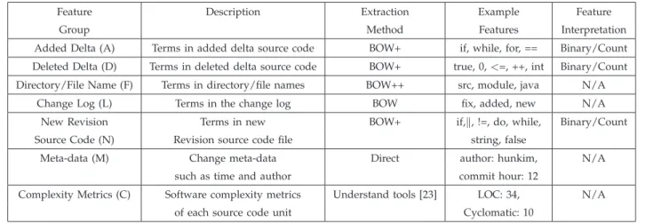
Fig. 1 summarizes the relative performance of the two classifiers and compares against the prior work of Kim et al [28]. Examining these figures, it is clear that feature selection significantly improves F-measure of bug predic-tion using change classificapredic-tion. As precision can often be increased at the cost of recall and vice versa, we compared classifiers using buggy F-measure. Good F-measures in-dicate overall result quality.

TABLE 5

The practical benefit of our result can be demonstrated by the following. For a given fixed level of recall, say 70 percent, our method provides 97 percent precision, while Kim et al. provide 52.5 percent precision. These numbers were calculated using buggy F-measure numbers from Table 5 and [28]. The buggy precision value was extra-polated from the buggy F-measure and the fixed recall figures. High precision with decent recall allows developers to use our solution with added confidence. This means that if a change is flagged as buggy, the change is very likely to actually be buggy.

Kim et al.’s results, shown in Fig. 1, are taken from [28]. In all but the following cases, this paper used the same corpus.

. This paper does not use Scarab and Bugzilla because those projects did not distinguish buggy and new features.

. This paper uses JCP, which was not in Kim et al.’s corpus.

Kim et al. did not perform feature selection and used substantially more features for each project. Table 4 reveals the drastic reduction in the average number of features per project when compared to Kim et al.’s work.

Additional benefits of the reduced feature set include better speeds of classification and scalability. As linear SVMs and Naive Bayes classifiers work in linear time for classification [25], removing 90 percent of features allows classifications to be done about 10 times faster. We have noted an order of magnitude improvement in code change classification time. This helps promote interactive use of the system within an Integrated Development Environment.

5.3 Statistical Analysis of Results

While the above results appear compelling, it is necessary to further analyze them to be sure that the results did not occur due to statistical anomalies. There are a few possible sources of anomaly.

. The 10-fold validation is an averaging of the results for F-measure, accuracy, and all of the stats presented. Its possible that the variance of the cross-validation folds is high.

. Statistical analysis is needed to confirm that a better performing classifier is indeed better after taking into account cross-validation variance.

To ease comparison of results against Kim et al. [28], the cross-validation random seed was set to the same value used by them. With the same datasets (except for JCP) and the same cross-validation random seed, but with far better buggy F-measure and accuracy results, the improvement over no feature selection is straightforward to demonstrate.

Showing that the Naive Bayes results are better than the SVM results when comparing Tables 5 and 6 is a more involved process that is outlined below. For the steps below, the better and worse classifiers are denoted, respectively, ascb and cw.

1. Increase the cross-validation cycle to 100 runs of 10-fold validation, with the seed being varied each run. 2. For each run, note the metric of interest, buggy F-measure, or accuracy. This process empirically Fig. 1. Classifier F-measure by project.

TABLE 6

generates a distribution for the metric of interest,

dmcb, using the better classifiercb.

3. Repeat steps 1, 2 for the worse classifier cw, attaining dmcw.

4. Use a one-sided Kolmogorov Smirnov test to show that the population CDF of distribution dmcb is larger than the CDF of dmcw at the 95 percent confidence level.

The seed is varied every run in order to change elements of the train and test sets. Note that the seed for each run is the same for bothcwandcb.

In step four above, one can consider using a two sample bootstrap test to show that the points of dmcb come from a distribution with a higher mean than the points ofdmcw[13]. However, the variance within 10-fold validation is the reason for the statistical analysis. The Birnbaum-Tingey one-sided contour analysis was used for the one-one-sided Kolmo-gorov-Smirnov test. It takes variance into account and can indicate if the CDF of one set of samples is larger than the CDF of the other set [9], [37]. It also returns a p-value for the assertion. The 95 percent confidence level was used.

Incidentally, step 1 is also similar to bootstrapping but uses further runs of cross validation to generate more data points. The goal is to ensure that the results of average error estimation via k-fold validation are not curtailed due to variance. Many more cross validation runs help generate an empirical distribution.

This test was performed on every dataset’s buggy F-measure and accuracy to compare the performance of the Naive Bayes classifier to the SVM. In most of the tests, the Naive Bayes dominated the SVM results in both accuracy and F-measure at p <0:001. A notable exception is the accuracy metric for the Gforge project.

While Tables 5 and 6 show that the Naive Bayes classifier has a 1 percent higher accuracy for Gforge, the empirical distribution for Gforge’s accuracy indicates that this is true only at apof 0.67, meaning that this is far from a statistically significant result. The other projects and the F-measure results for Gforge demonstrate the dominance of the Naive Bayes results over the SVM.

In spite of the results of Tables 4 and 5, it is not possible to confidently state that a binary representation performs better than count for both the Naive Bayes and SVM classifiers without performing a statistical analysis. Naive Bayes using binary features dominates over the perfor-mance of Naive Bayes with count features at a p <0:001. The binary SVM’s dominance over the best performing count SVM with the same feature selection technique (Gain Ratio) is also apparent, with ap <0:001on the accuracy and buggy F-measure for most projects, but lacking statistical significance on the buggy F-measure of Gaim.

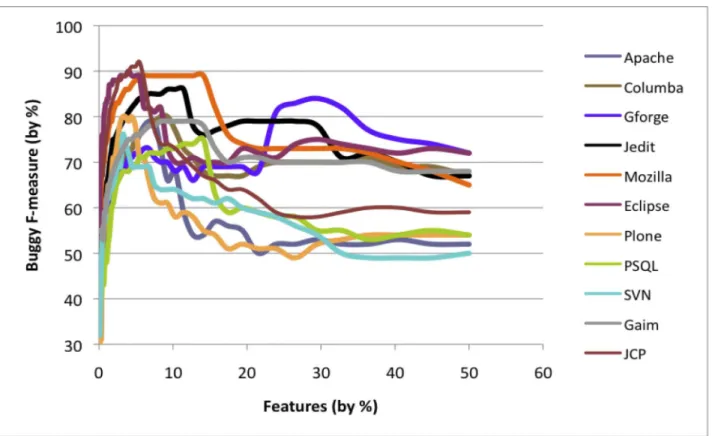
5.4 Feature Sensitivity

Research Question 3. Feature Sensitivity. What is the perfor-mance of change classification at varying percentages of features? What is the F-measure of the best performing classifier when using just 1 percent of all project features?

Section 5.2 reported results from using the best feature set chosen using a given optimization criteria, and showed that Naive Bayes with Significance Attribute feature

selection performed best with 7.95 percent of the original feature set, and SVM with Gain Ratio feature selection performed best at 10.08 percent. This is a useful result since the reduced feature set decreases prediction time as compared to Kim et al. A buggy/clean decision is based on about a tenth of the initial number of features. This raises the question of how performance of change classification behaves with varying percentages of features.

To explore this question, for each project we ran a modified version of the feature selection process described in Algorithm 1, in which only 10 percent (instead of 50 percent) of features are removed each iteration using Significance Attribute Evaluation. After each feature selec-tion step, buggy F-measure is computed using a Naive Bayes classifier.

The graph of buggy F-measure versus features, Fig. 2, follows a similar pattern for all projects. As the number of features decreases, the curve shows a steady increase in buggy F-measure. Some projects temporarily dip before an increase in F-measure occurs. Performance can increase with fewer features due to noise reduction but can also decrease with fewer features due to important features missing. The dip in F-measure that typically reverts to higher F-measure can be explained by the presence of correlated features which are removed in later iterations. While correlated features are present at the early stages of feature selection, their influence is limited by the presence of a large number of features. They have a more destructive effect toward the middle before being removed.

Following the curve in the direction of fewer features, most projects then stay at or near their maximum F-measure down to single digit percentages of features. This is significant since it suggests a small number of features might produce results that are close to those obtained using more features. The reason can be attributed to Menzies et al. [39], who state that a small number of features with different types of information can sometimes capture more information than many features of the same type. In the experiments of the current paper there are many feature types. Fewer features bring two benefits: a reduction in memory footprint and an increase in classification speed.

A notable exception is the Gforge project. When trimming by 50 percent of features at a time, Gforge’s optimal F-measure point (at around 35 percent) was missed. Feature selection is still useful for Gforge, but the optimal point seems to be a bit higher than for the other projects.

In practice, one will not know a priori the best percentage of features to use for bug prediction. Empirically from Fig. 2, a good starting point for bug prediction is at 15 percent of the total number of features for a project. One can certainly locate counterexamples including Gforge from this paper. Nevertheless, 15 percent of features is a reasonable practical recommendation if no additional information is available for a project.

To better characterize performance at low numbers of features, accuracy, buggy precision, and buggy recall are computed for all projects using just 1 percent of features (selected using the Significance Attribute Evaluation pro-cess). Results are presented in Table 7. When using 1 percent of overall features, it is still possible to achieve high buggy

precision, but at the cost of somewhat lower recall. Taking Apache as an example, using the F-measure optimal number of project features (6.25 percent, 1,098 total) achieves buggy precision of 0.99 and buggy recall of 0.63 (Table 5), while using 1 percent of all features yields buggy precision of 1 and buggy recall of 0.46 (Table 7).

These results indicate that a small number of features have strong predictive power for distinguishing between buggy and clean changes. An avenue of future work is to explore the degree to which these features have a causal

relationship with bugs. If a strong causal relationship exists, it might be possible to use these features as input to a static analysis of a software project. Static analysis violations spanning those keywords can then be prioritized for human review.

A natural question that follows is the breakdown of the top features. A software developer might ask which code attributes are the most effective predictors of bugs. The next section deals with an analysis of the top 100 features of each project.

5.5 Breakdown of Top 100 Features

Research Question 4. Best Performing Features.Which classes of features are the most useful for performing bug predictions? Table 8 provides a breakdown by category of the 100 most prominent features in each project. The top three types are purely keyword related. Adding further occur-rences of a keyword to a file has the highest chance of creating a bug, followed by deleting a keyword, followed finally by introducing an entirely new keyword to a file. Changelog features are the next most prominent set of features. These are features based on the changelog comments for a particular code change. Finally, filename features are present within the top 100 for a few of the projects. These features are generated from the actual names of files in a project.

It is somewhat surprising that complexity features do not make the top 100 feature list. The Apache project has three complexity features in the top 100 list. This was not presented in Table 8 as Apache is the only project where complexity metrics proved useful. Incidentally, the top individual feature for the Apache project is the average length of the comment lines in a code change.

TABLE 7

Naive Bayes with 1 Percent of All Features

The absence of metadata features in the top 100 list is also surprising. Author name, commit hour, and commit day do not seem to be significant in predicting bugs. The commit hour and commit day were converted to binary form before classifier analysis. It is possible that encoding new features using a combination of commit hour and day such as “Mornings,” “Evenings,” or “Weekday Nights” might provide more bug prediction value. An example would be if the hour 22 is not a good predictor of buggy code changes but hours 20-24 are jointly a strong predictor of buggy changes. In this case, encoding “Nights” as hours 20-24 would yield a new feature that is more effective at predicting buggy code changes.

Five of the 11 projects had BOW+ features among the top features, including Gforge, JCP, Plone, PSQL, and SVN. The Naive Bayes optimized feature (Table 5) contains BOW+ features for those projects with the addition of Gaim and Mozilla, a total of seven out of 11 projects. BOW+ features help add predictive value.

5.6 Algorithm Runtime Analysis

The classifiers used in the study consist of linear SVM and Naive Bayes. The theoretical training time for these classifiers has been analyzed in the research literature. Traditionally, Naive Bayes is faster to train than a linear SVM. The Naive Bayes classifier has a training runtime of

OðsnÞ, wheresis the number of nonzero features andnis the number of training instances. The SVM traditionally has a runtime of approximatelyOðsn2:1_{Þ[25]. There is recent}

work in reducing the runtime of linear SVMs toOðsnÞ[25]. Optimizing the classifiers for F-measure slows both down. In our experiments, training an F-measure opti-mized Naive Bayes classifier was faster than doing so for the SVM though the speeds were comparable when the number of features are low. The current paper uses Liblinear [15], one of the fastest implementations of a linear SVM. If a slower SVM package were used, the performance gap would be far wider. The change classifi-cation time for both classifiers is linear with the number of features returned after the training.

An important issue is the speed of classification on the projects without any feature selection. While the SVM or

Naive Bayes algorithms do not crash in the presence of a lot of data, training times and memory requirements are considerable. Feature selection allows one to reduce classification time. The time gain on classification is an order of magnitude improvement, as less than 10 percent of features are typically needed for improved classification performance. This allows individual code classifications to be scalable.

A rough wall-clock analysis of the time required to classify a single code change improved from a few seconds to a few hundred milliseconds when about 10 percent of features are used (with a 2.33 Ghz Intel Core 2 Quad CPU and 6 GB of RAM). Lowered RAM requirements allow multiple trained classifiers to operate simultaneously without exceeding the amount of physical RAM present in a change classification server. The combined impact of reduced classifier memory footprint and reduced classification time will permit a server-based classification service to support substantially more classi-fications per user.

The top performing filter methods themselves are quite fast. Significance Attribute Evaluation and Gain Ratio also operate linearly with respect to the number of training instances multiplied by the number of features. Rough wall-clock times show 4-5 seconds for the feature ranking process (with a 2.33 Ghz Intel Core 2 Quad CPU and 6 GB of RAM). It is only necessary to do this computation once when using these techniques within the feature selection process, Algorithm 1.

6

R

ELATED

W

ORK

Given a software project containing a set of program units (files, classes, methods or functions, or changes depending on prediction technique and language), a bug prediction algorithm outputs one of the following.

Totally ordered program units. A total ordering of program units from most to least bug prone [26] using an ordering metric such as predicted bug density for each file [44]. If desired, this can be used to create a partial ordering (see below).

Partially ordered program units. A partial ordering of program units into bug prone categories (e.g., the top

N percent most bug-prone files in [21], [29], [44])

Prediction on a given software unit. A prediction on whether a given software unit contains a bug. Prediction granularities range from an entire file or class [19], [22] to a single change (e.g., Change Classification [28]).

Change classification and faulty program unit detection techniques both aim to locate software defects, but differ in scope and resolution. While change classification focuses on changed entities, faulty module detection techniques do not need a changed entity. The pros of change classification include the following:

. Bug pinpointing at a low level of granularity, typically about 20 lines of code.

. Possibility of IDE integration, enabling a prediction immediately after code is committed.

. Understandability of buggy code prediction from the perspective of a developer.

TABLE 8

The cons include the following:

. Excess of features to account for when including keywords.

. Failure to address defects not related to recent file changes.

. Inability to organize a set of modules by likelihood of being defective.

Related work in each of these areas is detailed below. As this paper employs feature selection, related work on feature selection techniques is then addressed. This is followed by a comparison of the current paper’s results against similar work.

6.1 Totally Ordered Program Units

Khoshgoftaar and Allen have proposed a model to list modules according to software quality factors such as future fault density [26], [27]. The inputs to the model are software complexity metrics such as LOC, number of unique operators, and cyclomatic complexity. A stepwise multiregression is then performed to find weights for each factor. Briand et al. use object oriented metrics to predict classes which are likely to contain bugs. They used PCA in combination with logistic regression to predict fault prone classes [10]. Morasca and Ruhe use rough set theory and logistic regression to predict risky modules in commercial software [42]. Key inputs to their model include traditional metrics such as LOC, code block properties, in addition to subjective metrics such as module knowledge. Mockus and Weiss predict risky modules in software by using a regression algorithm and change measures such as the number of systems touched, the number of modules touched, the number of lines of added code, and the number of modification requests [41]. Ostrand et al. identify the top 20 percent of problematic files in a project [44]. Using future fault predictors and a negative binomial linear regression model, they predict the fault density of each file.

6.2 Partially Ordered Program Units

The previous section covered work which is based on total ordering of all program modules. This could be converted into a partially ordered program list, e.g., by presenting the topN percent of modules, as performed by Ostrand et al. above. This section deals with work that can only return a partial ordering of bug prone modules. Hassan and Holt use a caching algorithm to compute the set of fault-prone modules, called the top-10 list [21]. They use four factors to determine this list: software units that were most frequently modified, most recently modified, most frequently fixed, and most recently fixed. A recent study by Shihab et al. [48] investigates the impact of code and process metrics on future defects when applied on the Eclipse project. The focus is on reducing metrics to reach a much smaller, though statistically significant, set of metrics for computing potentially defective modules. Kim et al. proposed the bug cache algorithm to predict future faults based on previous fault localities [29]. In an empirical study of partially ordered faulty modules, Lessmann et al. [33] conclude that the choice of classifier may have a less profound impact on the prediction than previously thought, and recommend the ROC AUC as an accuracy indicator for comparative studies in software defect prediction.

6.3 Prediction on a Given Software Unit

Using decision trees and neural networks that employ object-oriented metrics as features, Gyimo´thy et al. [19] predict fault classes of the Mozilla project across several releases. Their buggy precision and recall are both about 70 percent, resulting in a buggy F-measure of 70 percent. Our buggy precision for the Mozilla project is around 100 percent (+30 percent) and recall is at 80 percent (+10 percent), resulting in a buggy F-measure of 89 percent (+19 percent). In addition, they predict faults at the class level of granularity (typically by file), while our level of granularity is by code change.

Aversano et al. [4] achieve 59 percent buggy precision and recall using KNN (K nearest neighbors) to locate faulty modules. Hata et al. [22] show that a technique used for spam filtering of e-mails can be successfully used on software modules to classify software as buggy or clean. However, they classify static code (such as the current contents of a file), while our approach classifies file changes. They achieve 63.9 percent precision, 79.8 percent recall, and 71 percent buggy F-measure on the best data points of source code history for two Eclipse plug-ins. We obtain buggy precision, recall, and F-measure figures of 100 percent (+36.1 percent), 78 percent (1:8 percent), and 87 percent (+16 percent), respectively, with our best performing technique on the Eclipse project (Table 5). Menzies et al. [39] achieve good results on their best projects. However, their average precision is low, ranging from a minimum of 2 percent and a median of 20 percent to a max of 70 percent. As mentioned in Section 3, to avoid optimizing on precision or recall, we present F-measure figures. A commonality we share with the work of Menzies et al. is their use of Information Gain (quite similar to the Gain Ratio that we use, as explained in Section 2.3) to rank features. Both Menzies and Hata focus on the file level of granularity.

Kim et al. show that using support vector machines on software revision history information can provide an average bug prediction accuracy of 78 percent, a buggy F-measure of 60 percent, and a precision and recall of 60 percent when tested on 12 open source projects [28]. Our corresponding results are an accuracy of 92 percent (+14 percent), a buggy F-measure of 81 percent (+21 per-cent), a precision of 97 percent (+37 perper-cent), and a recall of 70 percent (+10 percent). Elish and Elish [14] also used SVMs to predict buggy modules in software. Table 9 compares our results with that of earlier work. Hata, Aversano, and Menzies did not report overall accuracy in their results and focused on precision and recall results.

Recently, D’Ambros et al. [12] provided an extensive comparison of various bug prediction algorithms that operate at the file level using ROC AUC to compare algorithms. Wrapper Subset Evaluation is used sequentially to trim attribute size. They find that the top ROC AUC of 0.921 was achieved for the Eclipse project using the prediction approach of Moser et al. [43]. As a comparison, the results achieved using feature selection and change classification in the current paper achieved an ROC AUC for Eclipse of 0.94. While it’s not a significant difference, it does show that change classification after feature selection can provide results comparable to those of Moser et al., which are based on code metrics such as code churn, past bugs, refactorings, number of authors, file age, etc. An advantage of our change classification approach over that of

Moser et al. is that it operates at the granularity of code changes, which permits developers to receive faster feed-back on small regions of code. As well, since the top features are keywords (Section 5.5), it is easier to explain to developers the reason for a code change being diagnosed as buggy with a keyword diagnosis instead of providing metrics. It is easier to understand a code change being buggy due to having certain combinations of keywords instead of combination of source code metrics.

Challagulla et al. investigate machine learning algo-rithms to identify faulty real-time software modules [11]. They find that predicting the number of defects in a module is much harder than predicting whether a module is defective. They achieve best results using the Naive Bayes classifier. They conclude that “size” and “complexity” metrics are not sufficient attributes for accurate prediction. The next section moves on to work focusing on feature selection.

6.4 Feature Selection

Hall and Holmes [20] compare six different feature selection techniques when using the Naive Bayes and the C4.5 classifier [45]. Each dataset analyzed has about 100 features. The method and analysis based on iterative feature selection used in this paper is different from that of Hall and Holmes in that the present work involves substantially more features, coming from a different type of corpus (features coming from software projects). Many of the feature selection techniques used by Hall and Holmes are used in this paper.

Song et al. [51] propose a general defect prediction framework involving a data preprocessor, feature selection, and learning algorithms. They also note that small changes to data representation can have a major impact on the results of feature selection and defect prediction. This paper uses a different experimental setup due to the large number of features. However, some elements of this paper were adopted from Song et al., including cross validation during the feature ranking process for filter methods. In addition, the Naive Bayes classifier was used and the J48 classifier was attempted. The results for the latter are mentioned in Section 7. Their suggestion of using a log preprocessor is

hard to adopt for keyword changes and cannot be done on binary interpretations of keyword features. Forward and backward feature selection one attribute at a time is not a practical solution for large datasets.

Gao et al. [18] apply several feature selection algorithms to predict defective software modules for a large legacy telecommunications software system. Seven filter-based techniques and three subset selection search algorithms are employed. Removing 85 percent of software metric features does not adversely affect results, and in some cases improved results. The current paper uses keyword in-formation as features instead of product, process, and execution metrics. The current paper also uses historical data. Finally, 11 systems are examined instead of four when compared to that work. However, similarly to that work, a variety of feature selection techniques is used as well on a far larger set of attributes.

7

T

HREATS TO

V

ALIDITY

There are six major threats to the validity of this study.

7.1 Systems Examined Might Not Be Representative of Typical Projects

Eleven systems are examined, a quite high number compared to other work reported in literature. In spite of this, it is still possible that we accidentally chose systems that have better (or worse) than average bug classification accuracy. Since we intentionally chose systems that had some degree of linkage between change tracking systems and change log text (to determine fix inducing changes), there is a project selection bias.

7.2 Systems Are Mostly Open Source

The systems examined in this paper mostly all use an open source development methodology, with the exception of JCP, and hence might not be representative of typical development contexts, potentially affecting external validity [52]. It is possible that more deadline pressures, differing personnel turnover patterns, and varied development processes used in commercial development could lead to different buggy change patterns.

TABLE 9