Individual Claims Reserving: Using Machine Learning Methods

(1)

Individual Claims Reserving: Using Machine Learning

Methods

Dong Qiu

A Thesis

In

The Department

of

Mathematics and Statistics

Presented in Partial Fulfillment of the Requirements

for the Degree of Master of Science (Mathematics) at

Concordia University

Montreal, Quebec, Canada

December 2019

c

(2)

C

ONCORDIA

U

NIVERSITY

School of Graduate Studies

This is to certify that the thesis prepared

By: Dong Qiu

Entitled: Individual Claims Reserving: Using Machine Learning Methods

and submitted in partial fulfillment of the requirements for the degree of Master of Science (Mathematics)

complies with the regulations of this University and meets the accepted standards with respect to originality and quality.

Signed by the Final Examining Committee:

Chair Dr. Mélina Mailhot Examiner Dr. Frédéric Godin Examiner Dr. Mélina Mailhot Supervisor Dr. José Garrido Approved by

Dr. Cody Hyndman, Chair

Department of Mathematics & Statistics Date

Andr´e G. Roy, Dean Faculty of Arts and Science

(3)

Abstract

Individual Claims Reserving: Using Machine Learning Methods Dong Qiu

To date, most methods for loss reserving are still used on aggregate data arranged in a tri-angular form such as the Chain-Ladder (CL) method and the over-dispersed Poisson (ODP) method. With the booming of machine learning methods and the significant increment of computing power, the loss of information resulting from the aggregation of the individual claims data into accident and development year buckets is no longer justifiable. Machine learning methods like Neural Networks (NN) and Random Forest (RF) are then applied and the results are compared with the traditional methods on both simulated data and real data (aggregate at company level).

(4)

Acknowledgements

First of all, I devote my greatest thanks to my supervisor Dr. José Garrido for his guidance throughout my study at Concordia. Each and every time after our meeting, I felt inspired and had my hands full of content to learn. He is always patient and thoughtful, and his advice is pivotal. Without his valuable instruction, this paper would not have been finished smoothly.

I also want to express my sincere gratitude to all the other teachers in the past three years of my study - especially Dr. Mélina Mailhot and Dr. Frédéric Godin, for their sincere opinions on my thesis.

In addition, I would also like to thank my close friends, for their sustained encouragement during the whole process of writing, and my boss for understanding my situation and being supportive of my personal development.

Last but not least, I would like to thank my mom Min Chen and my dad Youqian Qiu for their everlasting love. Without their support, I would not have chance to study here and to chase my dreams.

(5)

List of Figures

3.1 Structure of Case Estimate Development Observations . . . 30

3.2 MLP Graphical Representation . . . 32

3.3 Graphical Representation of Cascading (Type 1) . . . 33

3.4 Decision Tree . . . 39

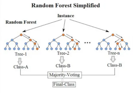
3.5 Random Forest . . . 42

3.6 Graphical Representation of Cascading (Type 2) . . . 43

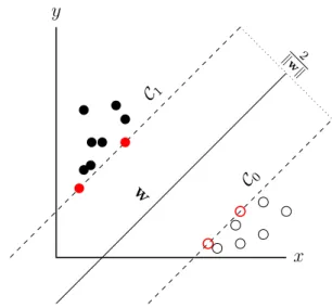
3.7 Graphical Representation of SVM . . . 45

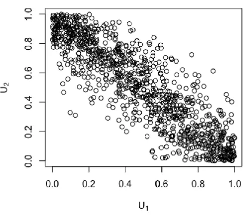
4.1 Frank Copula . . . 50

4.2 Graphical Prediction Comparison for Sample 3 . . . 60

4.5 Graphical Prediction Comparison for Sample c . . . 64

4.6 Graphical Prediction Comparison for Sample d . . . 64

4.7 Graphical Prediction Comparison for Sample e . . . 65

(8)

List of Tables

1 Claims Development Triangle . . . 2

1.1 Calculating CL Factors on Aggregate Data with CL Algorithm . . . 7

1.2 Prediction on Aggregate Data with CL Algorithm . . . 7

2.1 CL Factor and Variance from Sample 3 . . . 15

3.1 List of Most Common Kernel Functions. . . 47

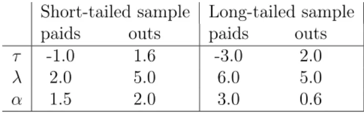
4.1 Calibration Parameters of Sample 1 and Sample 2 . . . 52

4.2 Allocation of Sample 1 and Sample 2 in Sample 3 . . . 53

4.5 Number of Claims in Each Accident Year . . . 56

4.6 Predictions for Sample 3 . . . 57

4.9 Running Time of Diﬀerent Methods . . . 62

4.10 Calibration Parameters of Sample a and Sample b . . . 63

4.11 Allocation of Sample a and Sample b in Sample e . . . 63

4.12 Comparison of loss reserve . . . 66

(9)

Introduction

In the case of non-life insurance, the related benefit is not paid to the insured necessarily as soon as the accident occurs, some years may pass between the actual occurrence and the final claim payment. There can be several reasons why the claim cannot be settled immediately, including further investigation, new information, court decisions, and so on.

This time gap is the reason why insurance companies must allocate sufficient loss reserves to cover any future payments for outstanding loss liabilities. To date, most methods for loss reserving still use aggregate data arranged in a triangular form, as shown in Table 1. Aggre-gate loss reserving data are placed in different cells for different accident and development years. Based on this, methods such as the Chain-Ladder (CL) or Bornhuetter-Ferguson (BF) algorithms are then applied to find some factors that can explain the development of payments from year to year, or to find the ultimate claims reserves at the finalization of the development period.

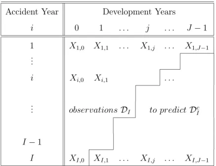
Wüthrich [2019] gives the notation of the aggregate claims reserves, where Xi,j

rep-resents the payments made for claims with accident year i in development year j, and

Ci,j = !jk=0Xi,k as the total payments made for claims with accident year i until

devel-opment year j. All the observations in the upper triangle are noted as _DI, and the lower

triangleDc

(10)

Accident Year Development Years i 0 1 . . . j . . . J ₋1 1 X1,0 X1,1 . . . X1,j . . . X1,J−1 ... i Xi,0 Xi,1 . . . ... observations_DI to predict DcI I₋1 I XI,0 XI,1 . . . XI,j . . . XI,J−1

Table 1: Claims Development Triangle

Later on, in order to know how much the real payments may deviate from the predictions, it was natural to set the CL model into a stochastic framework. For the CL method, according to Wüthrich [2019], many stochastic models were developed, including the distribution-free CL model, the over-dispersed Poisson (ODP) model with MLE parameter estimates, and the Bayesian CL model. In Taylor and McGuire [2016], some other models are mentioned (such as the EDF Mack model, cross-classified models).

Nonetheless, with the booming of machine learning methods, and the significant incre-ment of computing power, the loss of information resulting from the aggregation of the individual claims data into accident and development year buckets can now be prevented to a certain level. In Taylor et al. [2008], a GLM method is proposed to build the model for individual claim loss reserving in diﬀerent cases.

Due to the pattern recognition capabilities of neural networks, Harej et al. [2017] used these on long-tailed and short-tailed claims, for reserving and pricing of the simulated data introduced by Taylor et al. [2008] mentioned above. Long-tailed and short-tailed patterns are modeled by two log-normal distributions with diﬀerent parameters, and a copula is used to induce a dependence between them. There are 6,000 short-tailed claims and 4,000 long-tailed claims that are produced under this unified model. More samples are produced by

(11)

allocating diﬀerent numbers of claims from these two samples to each accident years. Then, we start with the same approach as Harej et al. [2017], by applying machine learning methods on simulated data, to which we add Random Forest (RF) along with a modified version of the cascading method. The RF method is one of the most accurate statistical learning algorithms available. It produces a highly accurate classifier for most datasets, and it runs eﬃciently on large databases. It corrects decision trees’ tendency to overfit their training set. Furthermore, instead of finding the development pattern of payments, the RF method puts the individual claims that have the same pattern or features into the same category and predicts the value by averaging all the values at the end node.

To eliminate the limitation of the cascading method, we found some approaches proposed by Aleandri [2017], by separating the predicting procedure into diﬀerent parts. It allows us to predict the closing delay time, the final amount of payments, and then individual loss reserving. However, in this thesis, due to the lack of real reserving data, we are not able to use them for comparison purposes.

(12)

Chapter 1 Classical Methods

1.1 Chain Ladder Algorithm

The Chain Ladder (CL) method consists in a deterministic algorithm, which is widely used to forecast future claim reserves. The main idea of the CL algorithm (see Wüthrich [2019]) is based on the assumption that for all accident years i, the cumulative payments behave according to the same pattern of changes in the sequence of the coming development years. For a given accident year i, and development year j, the cumulative payments have the following relation

Ci,j+1 ≈fjCi,j, i∈{1, ..., I}, j ∈{1, ..., J}, (1.1)

where the fj are called CL factors,age-to-age factors or link ratios.

Ultimately, we would like to know the cumulative claims reservesCi,J−1 for each accident

year, which can be calculated by equation ˆ Ci,JCL−1 =Ci,I−i J_"−2 j=I−i ˆ fjCL, with i > I −J+ 1, (1.2)

and more generally, _CˆCL

(13)

fj. In Wüthrich et al. [2010], estimators of fj are given as ˆ fCL j = !i∗₍_j₊₁₎ i=1 Ci,j+1 !i∗₍_j₊₁₎ i=1 Ci,j = i∗₍_j₊₁₎ $ i=1 Ci,j !i∗₍_j₊₁₎ n=1 Cn,j Ci,j+1 Ci,j , (1.3)

where i∗(j) = I −j is the last observed development year, which is the last diagonal

in the observed claims development triangle (See Table 1). If weights are added, then the weighted average CL factors can be represented by:

ˆ f_jCL = J−1 $ k=1 ωkjfˆik, (1.4)

where fij = C_Ci,j_i,j+1 and !iJ=1−jωij = 1. When ωij = !JC−i,jj

i=1 Ci,j, then the weighted average CL

factors in (1.4) reduce to those used in (1.3).

Easily we can calculate the total predicted CL reserve at time I for accident year i > I₋J+ 1, which is given as

ˆ

XiCL= ˆCi,JCL−1−Ci,I−i =Ci,I−i

% J_"−2 j=I−i ˆ fjCL−1 & . (1.5)

Therefore, the total yearly predicted claims in development year J for all accident years

can be written as:

ˆ RCL J = I $ i=1 ( ˆCi,J−Cˆi,J−1) = I $ i=1 (Ci,I−i J_"−1 j=I−i ˆ fjCL−Ci,I−i J−2 " j=I−i ˆ fjCL) = I $ i=1 Ci,I−ifˆJCL−1,

along with the total predicted claim reserve over all accident years, which is given by: ˆ RCL₌ $ i>I−J+1 ˆ RCL i . (1.6)

(14)

For example, Tables 1.1 and 1.2 use the synthetic data presented in Chapter 4 to illustrate the above formulas. They follow the steps of the CL algorithm by calculating the CL factors first; calculate the cumulative losses for the lower triangle; then compute the estimated loss reserves and compare them with the available data. The CL algorithm predicts overall reserves precisely when the claims are evenly distributed over diﬀerent development patterns or when the line of business is small; however, it performs poorly when the distribution of the patterns varies more.

A Robust General Multivariate Chain Ladder (GMCL) Method

A non-life insurance company typically divides portfolios intomcorrelated sub-portfolios,

wherem= 1, . . . , M andM is the total number of sub-portfolios, so that certain homogeneity

properties on each sub-portfolio are satisfied. The GMCL method is explained by Peremans et al. [2018]. The overall outstanding reserve R that will need to be paid in the future is

defined as: R= M $ m=1 I $ i=1 (C_i,J(m)−C_i,J(m₋)_i). (1.7)

Let Ci,j = (Ci,j(1), . . . , C

(M)

i,j ) denote the vector of cumulative claims of accident period i

and development period j for business linem. Consider the following model structure from

development period j toj + 1:

Ci,j+1 =Aj +BjCi,j+!i,j, i= 1, . . . , I, (1.8)

whereAj is theM vector containing the interceptsβ0(1),j, ...,β

(M)

0,j ,Bj is the theM×M matrix

that contains the development parameters β₁(m_,j), ...,β_M,j(m) for run-oﬀ triangle m in row j, and

!i,j = (#(1)i,j, ...,#

(M)

i,j ) are independent (over i) and symmetrically distributed random vectors

representing the error terms. Moreover, it is assumed that the errors !i,j satisfy

E[!i,j|Di,j] = 0,

Cov[!i,j|Di,j] =diag[Ci,j]1/2Σkdiag[Ci,j]1/2,

(1.9) whereDi,j is the set of cumulative claims for accident yeariup to and including development

(15)

A cc id en t Y ea r D ev el op m en t Y ea r (i n th ou sa nd ) 0 1 2 3 4 5 6 7 8 9 10 11 12 13 14 15 16 17 18 19 19 98 86 28 6 17 39 32 24 17 31 29 19 18 32 93 25 35 79 38 38 04 74 39 87 09 41 37 89 42 64 41 43 71 61 44 63 14 45 41 58 46 08 80 46 66 38 47 15 68 47 58 09 47 94 12 48 25 32 48 51 55 19 99 86 40 8 17 41 78 24 20 66 29 23 13 32 97 72 35 84 13 38 09 71 39 92 08 41 42 93 42 69 62 43 76 94 44 68 48 45 46 80 46 13 98 46 71 81 47 21 25 47 63 43 47 99 73 48 30 76 20 00 86 33 4 17 40 24 24 18 84 29 21 07 32 95 77 35 82 44 38 08 24 39 91 13 41 42 19 42 69 01 43 76 63 44 68 38 45 47 12 46 14 53 46 72 41 47 21 92 47 64 33 48 00 60 20 01 86 30 1 17 39 63 24 17 78 29 19 82 32 94 24 35 80 60 38 06 27 39 89 01 41 39 82 42 66 53 43 74 17 44 65 86 45 44 34 46 11 81 46 69 52 47 18 95 47 61 26 20 02 86 24 9 17 38 60 24 16 41 29 17 93 32 92 01 35 78 32 38 03 72 39 86 09 41 36 88 42 63 40 43 70 80 44 62 47 45 40 68 46 08 15 46 65 81 47 15 07 20 03 86 21 9 17 38 01 24 15 55 29 17 02 32 91 19 35 77 44 38 02 74 39 85 29 41 36 17 42 62 77 43 70 29 44 61 91 45 40 43 46 07 62 46 65 31 20 04 86 30 6 17 39 75 24 17 83 29 19 54 32 93 77 35 80 06 38 05 50 39 87 67 41 38 40 42 64 86 43 72 24 44 63 75 45 42 14 46 09 23 20 05 86 06 2 17 34 87 24 11 16 29 11 66 32 85 33 35 71 01 37 95 87 39 78 15 41 28 79 42 54 99 43 62 41 44 53 86 45 32 37 20 06 86 26 2 17 38 89 24 16 71 29 18 46 32 92 66 35 78 97 38 04 55 39 87 19 41 37 89 42 64 60 43 71 97 44 63 68 20 07 86 23 4 17 38 27 24 15 83 29 17 14 32 91 17 35 77 07 38 02 46 39 84 47 41 35 21 42 61 53 43 68 73 20 08 86 19 5 17 37 43 24 14 88 29 16 25 32 90 28 35 76 35 38 01 65 39 84 03 41 35 05 42 61 51 20 09 86 29 0 17 39 40 24 17 51 29 19 54 32 94 05 35 80 39 38 06 18 39 88 68 41 39 64 20 10 86 36 2 17 40 89 24 19 45 29 21 51 32 95 87 35 82 04 38 07 40 39 89 95 20 11 86 24 7 17 38 53 24 16 23 29 17 93 32 91 96 35 78 07 38 03 45 20 12 86 26 3 17 38 88 24 16 74 29 18 46 32 92 54 35 78 54 20 13 86 39 9 17 41 66 24 20 32 29 22 81 32 97 32 20 14 86 11 5 17 35 81 24 12 53 29 13 65 20 15 86 27 3 17 39 12 24 17 12 20 16 86 32 8 17 40 18 20 17 86 16 6 f C L j 2. 78 23 2. 41 45 2. 25 44 2. 17 72 2. 12 44 2. 09 58 2. 07 67 2. 06 09 2. 04 92 2. 04 19 2. 03 59 2. 02 74 2. 02 72 2. 02 08 2. 01 80 2. 01 60 2. 01 36 2. 01 07 0. 00 54 Ta bl e 1. 1: C al cu la ti ng C L Fa ct or s on A gg re ga te D at a w it h C L A lg or it hm cc id en t Y ea r D ev el op m en t Y ea r (i n th ou sa nd ) 0 1 2 3 4 5 6 7 8 9 10 11 12 13 14 15 16 17 18 19 P re di ct io n ˆ_X C L i R ea ld at a X C L i 19 98 0 0 19 99 48 57 02 26 25 26 24 20 00 48 31 74 48 58 01 57 40 57 71 20 01 47 97 46 48 28 58 48 54 82 93 55 93 71 20 02 47 57 35 47 93 52 48 24 61 48 50 84 13 57 7 13 58 1 20 03 47 14 65 47 56 93 47 93 10 48 24 19 48 50 41 18 51 0 18 54 1 20 04 46 66 94 47 16 30 47 58 60 47 94 78 48 25 88 48 52 11 24 28 7 24 27 8 20 05 45 99 50 46 57 08 47 06 34 47 48 55 47 84 65 48 15 69 48 41 86 30 94 9 30 99 8 20 06 45 42 13 46 09 40 46 67 11 47 16 48 47 58 78 47 94 96 48 26 06 48 52 29 38 86 1 38 88 5 20 07 44 60 27 45 38 66 46 05 88 46 63 55 47 12 87 47 55 14 47 91 29 48 22 37 48 48 58 47 98 5 47 95 5 20 08 43 68 85 44 60 39 45 38 79 46 06 01 46 63 68 47 13 01 47 55 28 47 91 43 48 22 51 48 48 72 58 72 1 58 77 7 20 09 42 66 25 43 73 71 44 65 36 45 43 84 46 11 14 46 68 87 47 18 25 47 60 57 47 96 76 48 27 87 48 54 11 71 44 7 71 54 1 20 10 41 40 91 42 67 56 43 75 05 44 66 72 45 45 23 46 12 55 46 70 30 47 19 70 47 62 03 47 98 23 48 29 35 48 55 60 86 56 5 86 42 8 20 11 39 85 85 41 36 65 42 63 17 43 70 55 44 62 13 45 40 56 46 07 81 46 65 49 47 14 84 47 57 13 47 93 29 48 24 38 48 50 61 10 47 15 10 47 08 20 12 38 03 95 39 86 37 41 37 19 42 63 73 43 71 12 44 62 71 45 41 15 46 08 41 46 66 11 47 15 46 47 57 75 47 93 92 48 25 02 48 51 24 12 72 70 12 72 13 20 13 35 83 91 38 09 66 39 92 35 41 43 40 42 70 13 43 77 69 44 69 41 45 47 97 46 15 33 46 73 11 47 22 54 47 64 89 48 01 12 48 32 26 48 58 52 15 61 20 15 59 84 20 14 32 87 22 35 72 94 37 98 00 39 80 13 41 30 71 42 57 05 43 64 28 44 55 73 45 34 04 46 01 20 46 58 80 47 08 08 47 50 30 47 86 42 48 17 46 48 43 65 19 29 99 19 33 05 20 15 29 18 91 32 93 15 35 79 38 38 04 85 39 87 31 41 38 17 42 64 73 43 72 16 44 63 77 45 42 22 46 09 50 46 67 21 47 16 57 47 58 87 47 95 05 48 26 16 48 52 39 24 35 26 24 33 57 20 16 24 18 54 29 20 62 32 95 08 35 81 48 38 07 08 39 89 65 41 40 59 42 67 23 43 74 72 44 66 39 45 44 89 46 12 20 46 69 94 47 19 34 47 61 67 47 97 86 48 28 98 48 55 23 31 15 05 31 16 55 20 17 17 36 92 24 14 01 29 15 15 32 88 91 35 74 78 37 99 95 39 82 18 41 32 84 42 59 24 43 66 53 44 58 02 45 36 37 46 03 56 46 61 20 47 10 50 47 52 75 47 88 88 48 19 94 48 46 14 39 84 47 39 84 97 f C L j 2. 78 23 2. 41 45 2. 25 44 2. 17 72 2. 12 44 2. 09 58 2. 07 67 2. 06 09 2. 04 92 2. 04 19 2. 03 59 2. 02 74 2. 02 72 2. 02 08 2. 01 80 2. 01 60 2. 01 36 2. 01 07 0. 00 54 ˆ_X C L19 43 21 2 X C L19 43 48 0 Ta bl e 1. 2: P re di ct io n on A gg re ga te D at a w it h C L A lg or it hm

(16)

year j, Σk is a symmetric positive definite M ×M matrix, and diag is the operator that

turns its arguments into a diagonal matrix.

Therefore, the parameters Aj, Bj and Σk are unknown model parameters and need to

be estimated from historical claims in order to predict future losses.

The Seemingly Unrelated Regression (SUR) model is then used based on (1.8). For historical claims only, the following system of equations is obtained

     y(1)_j ... y(_jM)     =      X(1)_j . . . 0 ... ... ... 0 . . . X(_jM)           β(1)_j ... β(_jM)     +      !(1)_j ... !(_jM)     , for i= 1, . . . , n(j) with n(j) = I−j, (1.10) where I is the latest accident period, j = 0,1,_{· · ·} , J₋1 for m = 1, . . . , M and where the

following holds true:

• y(_jm) = (C₁(m_,j₊₁) , . . . , C_n(m₍_j)₎_,j₊₁)′ _{is the} _n₍_j₎ _{vector of all observed losses at development}

period j+ 1 from triangle m;

• X(_jm) = ((1, C₁(_,jm))′_{, . . . ,}₍₁_{, C}(m)

n(j),j)′)′ is the n(j) ×(M + 1) matrix of the first n(j)

observations at development period j from each triangle, including the constant 1 as

the intercept Cm 0,j. Hence, X (1) j =. . . =X (M) j ;

• β(_jm) =(β₀(m_,j), . . . ,β_M,j(m))′ _{is the}_M _{+ 1}_{vector of development parameters of triangle} _m_,

including the intercept, here (β₀(m_,j), . . . ,β_M,j(m)) does not depend on subscript m, but it makes it easier to align with the rest part of the equation;

• !(_jm) = (#₁(m_,j), . . . ,#_n(m₍_j)₎_,j)′ _{is the} _n₍_j₎ _{vector of error terms of triangle}_m_.

The set of the firstn(j)claims up to and including development period j is presented as

Dj ={Ci,j|1≤i≤n(j), j ≤J−1}. From (1.9) it follows that

Cov[!j|Dj] =E[!j!′j|Dj] =diag[Cj]1/2(Σk⊗In(j))diag[Cj]1/2, (1.11)

where !j = (!(1) ′ j , . . . ,! (M)′ j )′, Cj = (C(1) ′ j , . . . ,C (M)′ j )′ with C (m)′ j = (C (m)′ 1,j , . . . , C (m)′ n(j),j) for

(17)

m = 1, ..., M, and _⊗ is the Kronecker product. Pre-multiplying both sides of Equation

(1.10) by diag[Ck]1/2 leads to the following linear regression model:

     y(1)_j ∗ ... y(_jM)∗     =      X(1)_j ∗ . . . 0 ... ... ... 0 . . . X(_jM)∗           β(1)_j ... β(_jM)     +      !(1)_j ∗ ... !(_jM)∗     , (1.12) withy(_jm)∗ =diag[C_k(m)]−1/2_y(m) j ,X (m)∗ j =diag[C (m) k ]−1/2X (m) j , and! (m)∗ j =diag[C (m) k ]−1/2! (m) j .

The generalized least squares (GLS) is an adaptation of least squares that can handle any type of correlation. Therefore, the estimator for the model in (1.12) becomes

ˆ

β_j = (X∗_j′)(Σ−_j1_⊗In(j))(X∗j)−1X∗

′

j (Σ−j1⊗In(j))y∗j, (1.13)

where X∗_j = diag[X(1)_j ∗, ...,X_j(M)∗] is a block diagonal matrix of size n(j)M ×M(M + 1), and y∗

j = (y(1)∗j , ...,y

(M)∗

j ). A feasible GLS (FGLS) estimator is usually introduced to

estimate the unknown Σj. FGLS replaces the unknown matrix Σj in (1.13) with Σˆj =

(ˆ!(1)∗_j , . . . ,ˆ!(_jM)∗)′_(ˆ_!(1)∗

j , . . . ,ˆ!

(M)∗

j )/n(j), whereˆ!

(m)∗

j are the residuals obtained from

estimat-ing (1.12) by least squares.

It has been shown that FGLS estimators in the GMCL model are very sensitive to outliers. Therefore, a robust methodology is then proposed by Peremans et al. [2018] for reserve estimates and outlier detection by combining robust SUR estimators with the GMCL model.

The system of equations in (1.12) can be rewritten as another linear regression model by reordering the equations. Let Y∗

i,j,X∗i,j and e∗i,j be the subvector or submatrix ofyj,Xj and

!∗

j respectively by extracting rows i, i+n(j), ..., i+n(j)(M −1).

Then the system of equations in (5) is equivalent to Y∗

i,j =X∗i,jβj+ei,j∗ , i= 1, ..., n(k). (1.14)

The Cov[e∗i,j|Di,j]can be easily obtained byΣj. Decompose the covariance matrixΣkinto

(18)

of the matrix |Γj|= 1.

Let e∗

i,j(b) be equal to Y∗i,j −X∗i,jb for any M(M + 1) vector b according to the SUR

representation in (1.14). Then, given an initial estimator of the scaleσˆj, the MM-estimators

( ˆβ_j,Γˆj) minimize 1 n(j) n(j) $ i=1 ρ   -e∗ i,j(b)′G−1e∗i,j(b) ˆ σk  , (1.15)

over all M(M + 1) vectors b and positive definite symmetric M _×M matrices G, where G

representsΓ, with the determinant of the matrix|G|= 1. The MM-estimator for covariance is defined as_Σˆ_j _{= ˆ}_σ2

jΓˆj. Evidently, takingρ(x) = x2 yields the iterated FGLS estimator. To

be robust against outliers, it is necessary to consider boundedρ functions. More specifically,

we assume that the function ρ satisfies the following conditions:

• ρ is symmetric, twice continuously diﬀerentiable and satisfies ρ(0) = 0;

• ρ is strictly increasing on [0, c] and constant on [c,∞] for some c >0.

The most favored family of ρfunctions for MM-estimators is the class of Tukey bi-square ρ functions given by ρ(x) =min(x2_/₂₋_x4_/₂_c2₊_x6_/₆_c4_{, c}2_/₆₎_{. Under the SUR model with}

normally distributed errors, the tuning parameterc >0is usually chosen to obtain a certain level of asymptotic eﬃciency. In the paper of Peremans et al. [2018], the Tukey bi-square ρ

function is always considered with tuning parameter c= 5.1229.

An initial estimator of scaleσˆkis required for MM-estimators. This scale estimator should

be robust in order for MM-estimators to be robust. Therefore, highly robust S-estimators have been introduced for SUR models to obtain a highly robust scale estimator.

Starting from the initial S-estimates, MM-estimates are computed simply by iterating the following estimating equations until convergence according to Maronna et al. [2006]:

ˆ βj = (X∗ ′ j )( ˆΣ −1 j ⊗Dn(j))X∗j)−1X∗ ′ j ( ˆΣ −1 j ⊗Dn(j))y∗j, ˆ Σj =M(e∗1,j( ˆβj), . . . ,e∗n(j),j( ˆβj))Dj( ˆβj), . . . ,e∗n(j),j( ˆβj))′ %_$n(j) i=1 ρ′(d1,j)di,j & ,

(19)

with Dj = diag[ω(d1,j), . . . ,ω(dn(j),j)], where ω(x) = ρ′(x)/x, di,j2 = e∗i,j( ˆβj)′Σˆ

−1

j e∗i,j( ˆβj),

and e∗

i,j( ˆβj) = Y∗i,j−X∗i,jβˆj are the residuals derived from the representation in (1.14).

1.2 Bornhuetter-Ferguson Algorithm

The Bornhuetter-Ferguson (BF) algorithm is similar to the CL algorithm, but it adds an assumption on prior informationµˆi for the expected ultimate claims of accident yeari. Once

we have a claims development pattern (γj)j=0,1,...,J−1, which is the proportion of total loss

for any accident year observed in development yearj, it will allow us to predict the reserves

using

ˆ

X_i,jBF _≈γjµˆi, (1.16)

under the normalization!J−1

j=0 γj = 1, and theγj have to be estimated based on observations.

An expert should give the prior information µˆi here instead of basing it on the past data

in DI, which is the claim reserve information we have from the upper triangle. Wüthrich

[2019] defines the following estimators for the development pattern, ˆ γ₀BF = ˆβ₀BF, (1.17) ˆ γjBF = ˆβjBF −βˆjBF−1, for j = 1, ..., J −2, (1.18) ˆ γ_jBF = 1−βˆ_JBF₋₂, (1.19) where βBF j = #J−2 l=j _fˆCL1 l = "j−1 l=o fˆlCL "J−2

l=0 fˆlCL. Therefore the ultimate claim estimate

ˆ

Ci,J−1, for

i > I ₋J+ 1, is estimated by the BF method ˆ CBF i,J−1 =Ci,I−i+ ˆµi J−1 $ j=I−i+1 ˆ γBF j =Ci,I−i+ ˆµi(1−βˆIBF−i), (1.20)

and then the claim reserve at time I for accident year i > I ₋J+ 1 is ˆ RBF i = ˆµi J−1 $ j=I−i+1 ˆ γjBF = ˆµi(1−βˆIBF−i). (1.21)

(20)

Finally the total outstanding loss liabilities would just be the sum of claim reserves from all accident years

ˆ RBF ₌ $ i>I−J+1 ˆ RBF i . (1.22)

No examples are given for the BF methods, since for the simulated data, no prior infor-mation by experts is available. However, a comparison of the CL and BF algorithms is given in Wüthrich [2019], which shows that they have the same structure:

ˆ

C_i,JCL₋₁ =Ci,I−i+ ˆCi,JCL−1(1−βˆIBF−i), (1.23)

ˆ

C_i,JBF₋₁ =Ci,I−i+ ˆµi(1−βˆIBF−i). (1.24)

The only diﬀerence is that for the BF method the external estimate µˆi is used for the

final claim and in the CL method, it is an observation based on the estimated _CˆCL i,J−1.

(21)

Chapter 2 Stochastic Methods

The previous chapter reviews some classical algorithms that provide ways to calculate the claim reserves, however as a measure of preciseness, there is also a need to validate the prediction uncertainty of these models.

In Wüthrich [2019], the conditional mean square error of prediction (MSEP) was used to validate model uncertainty. It is the most popular prediction uncertainty measure, and it can be calculated or estimated explicitly in many examples. Assume _Xˆ _{is a}_D_I_-measurable response variable for the random variable X. The conditional MSEP is defined by

msepX|DI( ˆX) =E[(X−Xˆ)2|DI], (2.1)

which can also be written as

msepX|DI( ˆX) =V(X|DI) + (E[X−Xˆ|DI])2, (2.2)

where in the righthand side of the equation, the first part is called process uncertainty, and the second part is called parameter estimation error or bias. In order to minimize the conditional MSEP, _Xˆ _{should be chosen such that its expected value is the same as}_E_[_X_|D_I_]_, if all parameters are known and if we can calculateE[X_|DI]. In other cases, E[X|DI] needs

to be estimated as accurately as possible, and the possible sources of parameter uncertainty in this estimation need to be determined.

(22)

In order to analyze this prediction uncertainty, the claim reserving algorithms must be set in a stochastic framework, which means the variables{Xi} have to be put into a family,

where each one is indexed by a parameter i, wherei belongs to some index set I, and it has

to be measurable with respect to some measurable space .S,! /.

Several stochastic methods are mentioned by Taylor and McGuire [2016] and by Wüthrich [2019], but only the following three main methods are reviewed here:

1. Mack models,

2. Cross-Classified models, 3. Bayesian CL models.

2.1 Mack Models

The non-parametric Mack model is the most basic of Mack models, which assumes the three following conditions:

(M1) Accident years are stochastic independent, i.e., incremental paymentsXi1,j1 and Xi2,j2

are independent if i1 ∕=i2,

(M2) for eachi, cumulative payments Ci,j form a Markov process, asj varies,

(M3) there exist fj >0, j ∈{0, ..., J −1}, and σj2 > 0, j ∈ {0, ..., J −1}, such that for all

i_∈_{1, ..., I_} and j _∈_{1, ..., J ₋1_}, (a) E[Ci,j+1|Ci,j] =fjCi,j,

(b) V[Ci,j+1|Ci,j] =σj2Ci,j.

As we can see from these three conditions, and comparing to the previous CL algorithm, it is a stochastic model in the sense that it considers both expected values (fj) and the

variances (σj) of observations and the reason why it is called distribution-free is that it does

not assume a known distribution for the observations, we will see the diﬀerence later when introducing other models.

(23)

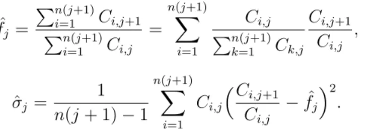
ˆ fj = !n(j+1) i=1 Ci,j+1 !n(j+1) i=1 Ci,j = n_$(j+1) i=1 Ci,j !n(j+1) k=1 Ck,j Ci,j+1 Ci,j , (2.3) ˆ σj = 1 n(j+ 1)₋1 n(_$j+1) i=1 Ci,j %_C i,j+1 Ci,j − ˆ fj &2 . (2.4)

By adding the variance, it makes it possible to compute the MSEP for _Cˆ _{using (2.2). In} this case,

msepC|DI( ˆC) = V(C|DI) + (E[C|DI]−Cˆ)2, (2.5)

where E[X_|DI]−Xˆ = 0. By using (M3b) recursively, (2.5) can be written as

msepC|DI( ˆC) =V(C|DI) = I $ i=2 % Ci,I−i J_"−2 j=I−i σ_j2). (2.6)

The CL factor and variance can be calculated using (2.3) and (2.4), except for the last variance since there will not be enough information. According to Mack [1993], if _fˆ_J

−2 = 1

and if the claims development is believed to be finished after J − 2 years, we can put ˆ

σJ−2 = 0. If not, we extrapolate the usually exponentially decreasing series σ1, ...,σJ−4,σJ−3

by one additional member, for instance by log-linear regression or more simply by requiring that σJ−4/σJ−3 = σJ−3/σJ−2 holds at least as long as σJ−4 > σJ−3. This last possibility

leads to: ˆ σJ−2 =min{ ˆ σ4 J−3 ˆ σ2 J−4 ; ˆσ_J2₋₃; ˆσ_J2₋₄_}. (2.7)

Table 2.1 gives an example of the calculation of CL factors and variances for the data in Sample 3, which will be defined later in Chapter 4.

0 1 2 3 4 5 6 7 8 9 10 fCL j 2.0163 1.3896 1.2077 1.1285 1.0864 1.0631 1.0483 1.0372 1.0308 1.0252 1.0214 σj 872.84 479.32 797.58 875.44 531.01 318.07 685.87 384.31 393.44 403.36 632.96 11 12 13 14 15 16 17 18 msep 1.0177 1.0140 1.0123 1.0104 1.0094 1.0078 1.0083 1.0046 -948.43 809.23 1760.62 1067.58 684.23 441.54 9.38 1.00 6,313,104,379.62

Table 2.1: CL Factor and Variance from Sample 3

(24)

of this non-parametric Mack model: one of them is called Exponential Dispersion Family parametric Mack model (EDF Mack model), which simply replaces (M3b) above with a dis-tributional assumption Xi,j+1|Ci,j ∼ EDF(δij,φij;a, b, c). The form of the variance allowed

in the EDF Mack model is more general than in the non-parametric Mack model. The other extension is called Over-Dispersed Poisson (ODP) Mack model, which replaces (M3b) with another distributional assumption Xi,j+1|Ci,j ∼ODP(µij,φij).

According to Taylor and McGuire [2016], under the assumption of the ODP Mack model, and if in addition the dispersion parameters φij are just column dependent (φij =φj), then

the _fˆ_j _{from (2.3) are minimum variance unbiased estimators (MVUEs) of the} _f_j_{. The} _Cˆ_i,j and _Xˆ_{, under the same condition are also MVUEs of} _C_i,j _and _X_.

This MVUE result is much stronger than the non-parametric Mack model that was referred to in the previous section, as the estimators here are minimum variance out of all unbiased estimators, not just out of the linear combinations of the _fˆ_j_.

With the definition above, the parameter estimates of the ODP Mack model can be calculated using the maximum likelihood method. However, Strascia and Tripodi [2018] used another method called quasi-likelihood function, which is defined by Wedderburn [1971] by specifying only the relation between mean and variance as follow:

k(Xi,j,φ) µi,j = Xi,j −µi,j V(µi,j) , (2.8) or equivalently, k(Xi,j,φ) = 0 µij Xij Xij −s φV(s) ds. (2.9)

Therefore over all Xi,j, the quasi-likelihood function can be written as,

K(X;β,φ) = $ i+j≤t ωij k(Xi,j;β,φ) = $ i+j≤t ωij 0 µij Xij Xij −s φV(s) ds, (2.10)

where µi,j depends on β – the parameter estimates of this model. φ is the dispersion

pa-rameter independent from i and j, ωi,j is the weight on each K(Xi,j;β,φ). t is introduced

by Strascia and Tripodi [2018] as the balance-sheet year, all the data before tis known with

(25)

the so-called variance function of the GLM, andh=g−1_{, where}_g _{is the link function.}

Maxi-mizing this equation can be used to estimate theβ parameters, due to the similar properties

it has with the likelihood function.

In the ODP model with a logarithmic link-function instead, the relation between mean and variance is the following:

E[Xi,j+1|Ci,j] =µij =ec+ai+bj and V[Xi,j+1|Ci,j] =φV(µij) =φµij. (2.11)

By inserting these equations into (2.8), the expression of the quasi-likelihood function for the ODP model can be written as:

K(X;β,φ) = $ i+j≤t ωij φ 1 Xijlog µij Xij − µij +Xij 2 , (2.12)

the _βˆ _{estimate is calculated by searching for the} _β _{= (}_{c, a}₁_{, . . . , a}_I_{, b}₁_{, . . . , b}_J₎⊤ _{values that}

maximize Function K in (2.10), so that the observed data is the most probable. The opti-mization problem can be solved through the Gauss-Newton method.

One method often used to estimate the observed data model goodness of fit is to analyze the generalized Pearson residuals. In the ODP case, with ωij = 1, the residuals are:

rij = Xij −µˆij -ˆ φµˆij , (2.13)

where _φˆ _{can be calculated through Pearson estimator} _φˆ₌ 1

n−p

!

i+j≥tωij(Xij−µˆij)

2

V( ˆµij) , n−p is

the number of the model degrees of freedom, n is the number of the observed data, p is the

number of parameters to be estimated. Pearson statistics χ2 ₌ !

i+j≤tωij

Xij−ˆµij

V(ˆµij) is used in Strascia and Tripodi [2018] to

cal-culate the overall discrepancy between empirical and theoretical data. Under the quasi-likelihood case, the deviance is:

(26)

Finally, according to Strascia and Tripodi [2018], for the ODP Mack Model, it is possible to calculate the MSEP for total reserve R with the following more compact form:

msepX|DI( ˆR) = ˆφ $ i+j>t ˆ µij + $ i+j>t ˆ µ2_ijx⊤_ijVˆ[ ˆβ]xij + $ i1+j1>t i2+j2>t (i1,j1)∕=(i2,j2) ˆ µij1µˆij2x⊤i1,j1Vˆ[ ˆβ]xi2,j2, (2.15)

where xi,j is the dummy variables vector, which is used to code accident and development

year.

Another concept is introduced by Strascia and Tripodi [2018] which is the Claims De-velopment Result; it calculates if the claims reserve estimate in year t for accident year i is

enough to pay the claims for the next year and new claims reserve at the next yeart+ 1:

CDRi,t+1 = ˆCi,J(t)−Cˆ

(t+1)

i,J , (2.16)

where _Cˆ(t)

i,J is the ultimate cost estimate at time t for claims from accident year i. Here t is

used as the superscript instead of usingm , which was used to represent the diﬀerent line of

business earlier.

Particularly, it is a loss for the insurance company if CDRi,t+1 < 0, while it is a gain

with a positive result.

In the chain ladder framework, the CDRi,t+1 is written in the following way:

! CDRi,t+1 = ˆCi,J(t)−Cˆ (t+1) i,J =Ci,t−i % J_"−1 j=t−i ˆ

f_j(t)&%1₋Ci,t−i+1/Ci,t−i ˆ f_t(₋t)_i J_"−1 j=t−i+1 ˆ f_j(t+1) ˆ f_j(t) & . (2.17)

By adding a credibility factorα_j(t) = Ct−j,j

!t−j

i=1Cij, the ratio between two link ratios associated

with the same j development year and estimated in a two-years-in-a-row balance sheet can

be written as: ˆ f_j(t+1) ˆ f_j(t) =α (t) j Ct−j,j+1/Ct−j,j ˆ f_j(t) + (1−α (t) j ). (2.18)

(27)

the following way: ! CDRi,t+1 = ˆCi,J(t)−Cˆ (t) i,J Ci,t−i+1/Ci,t−i ˆ f_t(₋t)_i J_"−1 j=t−i+1 % α(_jt)Ct−j,j+1/Ct−j,j ˆ f_j(t) + (1−α (t) j ) & . (2.19)

Another additive loss reserving model for the multi-year non-life insurance risk was de-veloped by Diers and Linde [2013], which is to elaborate on the risk modelling for non-life insurance companies by modelling insurance risk in a multi-year context. It is recommended to use this formula in case of attritional claims such as homogeneous and stable portfolios. However, for large claims, it should be modelled separately. Hahn [2017] also extended this model onto dependent lines of business by adding weights and covariance matrix.

2.2 Cross-Classified Model

Referred to as EDF cross-classified model (Taylor and McGuire [2016]), it is defined as: (EDFCC1) The random variables Xij ∈DI are stochastically independent.

(EDFCC2) Fori= 1,2, ..., I, and j = 1,2, ...J

(a) Xij ∼EDF(µij,φij;a, b, c), φij are dispersion parameters,

(b) E[Xij] =µij =αiβj for some parameters αi,βj >0, and,

(c) !J

j=1βj = 1.

Comparing to the regular Mack model (i.e. non-parametric Mack model), instead of having only fj as a parameter, this model uses αi and βj as parameters for both row and

column eﬀects on the expected value ofXij, we can regardαias the ultimate claim reserve for

accident yeari, andβj as the portion of this total claim reserve amount in each development

yearj, which is similar to the assumption of the BF algorithm, but without prior information

given by experts. It is obvious that regular Mack models apply to cumulative data, whereas cross-classified models apply to incremental data, which implies that the cross-classified model is more general.

(28)

If the modified (EDF CC2a), (EDF CC2b) are as in ODP form, which is the sub-family

of EDF cross-classified family, along with the further condition φij = φ, then it can be

rewritten as

Xij ∼ODP(αiβj,φ) = ODP(µij,φ), (2.20)

where

µij =exp(lnαi+ lnβj). (2.21)

This modified model is called over-dispersed Poisson (ODP) cross-classified model. Wüthrich [2019] gives more details about this model, where

Xij

φ ∼P oi( αiβj

φ ), (2.22)

and we observe that,

E[Xij] =αiβj, (2.23)

V(Xij) = φαiβj. (2.24)

Two side constraints are commonly used in order to make the parameters αi and βj

uniquely identifiable, which are

α1 = 1 or

J−2

$

j=1

βj = 1. (2.25)

The first option is more convenient in the application of GLM methods, the second option gives an explicit meaning to the pattern (β1,β2, . . . ,βJ−2), namely, that it corresponds to

the cash flow pattern.

The best-estimate reserves at time I are given by

ˆ X = $ i+j>I E[Xij|DI] = $ i+j>I αiβj, (2.26)

(29)

Then the MLE estimates of αi and βj are given by ˆ αM LE_i = ˆC_i,JCL₋₁ and βˆ_jM LE =%1₋ 1 ˆ fCL j−1 &J_"−2 k=j 1 ˆ fCL k , (2.27)

for i= 1, . . . , I and j = 1, . . . , J ₋1. Moreover,βˆM LE

0 =

#J−2

k=0 _fˆCL1

k .

Since _CˆCL

i,J−1 is the estimator for αˆi, and !jJ=1−2βj = 1, on the overall level, the results

should be almost the same as the results of the CL Mack model, but for the prediction of payments for each development year, the results will show some diﬀerences.

2.3 Bayesian CL Model

Wüthrich [2019] gives the gamma-gamma Bayesian CL model, which belongs to the exponential dispersion family (EDF) with conjugate priors. The advantage of this model is that the posterior distribution can be calculated analytically, which allows that all quantities of interest be determined in closed form.

Assume that giving fixed constants σj >0, and j = 0, ..., J −2, the Bayesian CL model

is defined as:

(a) Conditionally, given Θ = (θ0, . . . ,θJ−2), the Ci,j are independent (in i) Markov

processes (in j) with conditional distributions, Fi,j+1 =

Ci,j+1

Ci,j

3 3

3Ci,j,Θ∼Γ(Ci,jσj−2,θjCi,jσ−j2). (2.28)

(b) θj are independent and Γ(γj, fj(γj −1))-distributed with given prior constants

fj >0,γj >1.

(c) Θ and Ci,0 are independent and Ci,0 >0, P-a.s.

For a given parameter Θ, the conditional mean is given by

(30)

From this, it can be found that θ_j−1 plays the role of the CL factor fj here. The reason

for choosing the prior parameters of the distribution of θj is that

E[θ_j−1] = 1

γj−1

fj(γj −1) =fj. (2.30)

where the γj here is diﬀerent from the γ from equation (1.16).

Recall that the corresponding probability density function in the shape-rate parametriza-tion for the gamma distribuparametriza-tion Γ(α,β) is

f(x;α,β) = β

α_xα−1_e−βx

Γ(α) , (2.31)

where Γ(α) = 4₀∞xα−1_e−x_dx _{is the gamma function, when} _α _{is a complex number with a}

positive real part, while Γ(α) = (α₋1)! when α is a positive integer.

Then the joint likelihood function of the observations DI and the parameters Θis given

by h(DI,Θ) = " (i,j)∈II,j>1 (θj−1Ci,j−1 σ2 j−1 ) Ci,j−1 σ2_j₋₁ Γ(Ci,j−1 σ2 j−1 ) F Ci,j−1 σ_j2₋₁ −1 i,j exp{− θj−1Ci,j−1 σ2 j−1 Fi,j} ×g(C1,0, ..., CI,0) J_"−2 0 (fj(γj −1))γj Γ(γj) θγj−1 j exp{−θjfj(γj −1)}, (2.32)

where II is the index set of observations DI, and g(C1,0, ..., CI,0) denotes the density of the

first column j = 0.

This allows to apply Bayes rule which provides the posterior of Θ, conditionally given

DI, h(Θ_|DI)∝ J−2 " j=0 θ γj+!I_i₌₁−j−1Ci,j_σ2 j − 1 j e −θj 5 fj(γj−1)+!Ii=1−j−1 Ci,j+1 σ2_j 6 (2.33) which in turn proves that

Θ_|DI ∼Γ 7 γj+ I−_$j−1 i=1 Ci,j σ2 j , fj(γj −1) + I−_$j−1 i=1 Ci,j+1 σ2 j 8 . (2.34)

(31)

Under the assumptions of a gamma-gamma Bayesian CL model, the posterior Bayesian CL factors are given by

ˆ

f_jBCL=E[θ−_j1_|DI] =αjfˆjCL+ (1−αj)fj, (2.35)

with CL factor estimate _fˆCL

j given by (1.3) and credibility weight

αj = !I−J−1 i=1 Ci,j !I−J−1 i=1 Ci,j+σ2j(γj −1) ∈(0,1). (2.36)

Therefore, the prediction for the accumulative payment for accident yeariwithi+J−1> I is

ˆ

C_i,JBCL₋₁ =E[Ci,J−1|DI] =Ci,I−i J_"−2

j=I−i

ˆ

f_jBCL. (2.37)

Consider the gamma-gamma Bayesian CL model with a non-informative prior γj → 1,

it is obvious that αj = 1in this case, and therefore fˆjBCL= ˆfjCL and Cˆi,JBCL−1 = ˆCi,JCL−1, which

implies that the CL model is a special case of the Bayesian CL model. For the conditional MSEP obtained earlier,

msepCi,J−1|DI( ˆC

BCL

i,J−1) = V(Ci,J−1|DI) + (E[Ci,J−1|DI]−Cˆi,JBCL−1)2

=V(Ci,J−1|DI).

(2.38) This shows the optimality of the Bayesian CL predictor within the model, and that what remains is the calculation of the conditional variance of the final claim.

Wüthrich [2019] gives the solution for conditional MSEP as:

BCL

i,J−1) = ˆCi,JBCL−1ΓI−i+ ( ˆCi,JBCL−1)2∆I−i,

msepCi,J−1|DI( $ i ˆ CBCL i,J−1) = $ i

BCL i,J−1) + 2 $ i<l ˆ CBCL i,J−1Cˆl,JBCL−1∆I−i, (2.39)

(32)

where Γk and ∆k are defined as Γk= J−2 $ j=k σ2_j J_"−2 n=j % ˆ f_nBCLσ 2 n(γn−1) +!Ii=1−n−1Ci,n σ2 n(γn−2) +!I_i₌₁−n−1Ci,n & , ∆k = J−2 " j=k %_σ2 n(γn−1) +!Ii=1−n−1Ci,n σ2 n(γn−2) +!Ii=1−n−1Ci,n & −1. (2.40)

Wüthrich [2019] also discovered that in the non-informative prior case, γj → 1, the

approximation of msepCi,J−1|DI with non-informative priors and Mack’s formula are very

close. For many typical non-life insurance data sets, this observation still holds true and it suggests the use of the simpler formula.

There are many other stochastic methods, however they still share same pitfalls when applied to actual data. Therefore, Hartl [2014] provides a way to improve the performance of triangle GLMs using splitlinear rescaling and parametric resampling with a limited Pareto distribution. Meyers [2016] describes a method to fit a bivariate stochastic model that cap-tures the dependencies between the two lines of insurance, given a Bayesian Markov chain Monte Carlo (MCMC) stochastic loss reserve model. Also, Korn [2015] gives some strategies on loss development modelling with curve fitting, credibility, and layer adjustments. Lally and Hartman [2018] applied Gaussian Process (GP) regression with input warping and sev-eral covariance functions for loss reserving prediction, which requires little input from the modeller.

Mulquiney [2006] applied artificial neural networks on loss reserves triangle data. Fur-therer more, Jamal [2018] applied more machine learning methods on loss reserves triangle data, including random forest, neural network, gradient boosting machine and a boosted Tweedie compound poisson model.

(33)

Chapter 3 Individual Claim Reserving

The previous methods described above all focus on using the aggregate data triangle for loss reserving, assuming that insureds are independent. However, in real life, they are not necessarily independent, and there are diﬀerent types of dependency between the claims of diﬀerent insured. With the computational power we have now, it would be more accurate to predict the claim reserve of each insured separately without losing the dependence be-tween claims, and then aggregate the claim reserves to produce the aggregate claim reserves prediction.

So as not to confuse it with aggregate claim reserving methods, here each individual claim payment is denoted as xm

i,j, where m is the index of each insured, m ∈ M = {1,2, . . . , M},

and i is the accident year, while j is the development year. Here each claim must have a

fixed accident year, therefore the combinations of m and i are prescient.

Naturally, the aggregate claim reserve Xi,j can be written as:

Xi,j =

$

m∈Φ(i)

xm_i,j, (3.1)

where Φ(i) = {m(1)_i , m(2)_i , ..., m(_in), ..., mNi

i } is the set of claims incurred in accident year i,

m(_in) _∈ M, n = 1,2, ..., Ni, where Ni is the maximum number of claims in accident year i.

(34)

written as cm_i,j = j $ k=1 xm_i,k. (3.2)

Then the cumulative aggregate claim reserve can be written as:

Ci,j = j $ k=1 Xi,k = j $ k=1 $ m∈Φ(i) xm_i,k = $ m∈Φ(i) cm_i,j. (3.3)

Here our ultimate goal is to find a model that can predict each unknown xm

i,j in the lower

triangle, knowing that here the total reserve for the most recent year can be calculated by

R= I $ i=1 Xi,J−i+1 = I $ i=1 $ m∈Φ(i) xm_i,J₋_i₊₁. (3.4)

3.1 GLM Individual Claim Reserving Methods

In some companies, actuaries have already started using GLM methods to predict indi-vidual claim loss reserving.

Taylor et al. [2008] provides various forms of individual claim reserving models, showing how these methods perform more eﬃciently than aggregate models. To establish an individ-ual model, let ym _{be the response of interest for the}_m_{-th claim, and use} _vm _{instead of} _X

m

(to avoid being confused with aggregate reserve data Xi,j) to be the covariate vector for the

m-th claim. It has the following basic form:

ym _∼F(_·;vm,β), (3.5)

where F is some specific distribution function, β is a vector of parameters which are

inde-pendent of the claims and needs to be estimated. Denote

gm =E[ym], (3.6)

(35)

gm =g(vm,β), (3.7)

for some unique function g. vm _{can also be decomposed into three general parts as} _vm(S)_,

vm(T)_{, and} _vm(U) _{that stand for static, time, and unpredictable covariate vectors.}

For the individual claim models that are only dependent on time covariates, there is a more obvious way to separate the time covariates into diﬀerent components, namely

am _{= accident period;}

dm _{= development period when the claim finalized;}

pm ₌_am₊_dm _{= experience period in which the claim finalization occurs;}

tm _{= operational time, which maps development time} _δ _{to an interval [0,1],}

where in each case the superscript m indicates that the value of the time variable concerned

is that observed for the m-th claim.

Here we changed the notation for operational time t as tm₍_δ_{) =} !N i=1

I{τi≤δ}

N , where I

is an indicator function, τi is the finalization time for claim i, and this definition gives the

proportion of incurred claims that are finalized at or before that time (δ), for a given but

arbitrary accident year, with N claims incurred.

Taylor et al. [2008] also explains that the model depends only onam _and_tm_{, or else time}

related quantities other thanam _and _tm_{, do not require statistical case estimation (in short,}

statistical case estimation consists of estimating the ultimate cost of each claim). At the same time, depending on unpredictable covariates will make the model more complicated and will require to average the forecast; Therefore, the best model here would be one depending only on time and static covariates, as its forecast can be put into statistical case estimate form.

For a single accident period a, the model used to predict the m-th claim’s loss reserve

would now be:

y∗m ₌

0

(36)

• the * in y∗m _{represents that its value is a forecast;}

• the integral is only over pm _because _a _{is a single period,} _tm _{depends on} _pm _{only, and}

v∗m(S) _{is static;}

• g(·)is the statistical case estimate in respect of them-th unfinalised claim, conditional

ona,tm _, _pm _,_v∗m(S)_;

• the ∗ inv∗m(S) _{means that its response will only be observable in the future;}

• tm _{is the mapping of real-time} _pm _{to operational time;}

• and the measure P(·) onpm _{may now depend on} _v∗m(S)_.

This is equivalent to the GLM form which is usually known as: g(y∗m_{) =}_vmT_βˆ_{, where}

g(·) is the link function, βˆ is a vector of estimated parameters, and the upper T denotes

vector or matrix transposition, and here vm _{can be decomposed into (}_a_, _tm_, _pm_,_v∗m(S)_).

Actuaries see the models discussed above as “paid” models, for the reason that they only depend on paid losses. The insurer’s various estimates of these losses through the lifetimes of the claims are not taken into consideration at all.

Another model which is usually referred to as “incurreds” model is a conventional alter-native form of model forecasts for ultimate losses on the basis of the insurer’s estimates at the valuation date. A statistical case estimation form of this is also considered in Taylor et al. [2008].

In the following, the term case estimate will be used to mean a subjective estimate of the ultimate incurred loss placed by an insurer on an individual claim. The estimate will usually be made by a claims assessor and is often referred to as a real estimate or manual estimate, where each claim involves a whole sequence of case estimates through its lifetime. The factor relating case estimates and the ultimate incurred cost is considered as the general thrust of a model, and it is usually represented by a ratio referred to as the age-to-ultimate ratio, defined as:

R:Age-to-ultimate ratio = U :Expected ultimate incurred loss

(37)

where the “Expected” in the numerator is used in its statistical sense. A model like this will be referred to as a case estimates model. It corresponds to the conventional “incurreds” model.

However, the possibility of a zero numerator or denominator in (3.7) complicates the model, with the result that the model needs to consist of some sub-models, where I denotes

the current case estimate, U denotes the ultimate incurred loss, therefore R = U/I. Here F(.)denotes a distribution function.

More specifically, three sub-models are required:

• Sub-Model 1: P[U = 0],

• Sub-Model 2: F(U_|I = 0, U >0),

• Sub-Model 3: F(R|I >0, U >0).

Because in the case I = 0, the ratio R does not exist, and so the size of U must be

modeled directly, rather than asU =I_×R, cases I = 0and I _∕= 0 are dealt with separately, as are the cases U = 0 and U ∕= 0. Moreover, the distribution of U, with a discrete mass

at U = 0, is best modeled by recognizing separately the mass and the remainder of the distribution (assumed continuous).

Under this model, the statistical case estimate for U is:

E[U] =E[U|U ∕= 0]P[U ∕= 0]. (3.10)

Consider a claim from accident period a, reported in development period r, and finalized

in development periodf, which is not the same as CL factor. It will carry a case estimateId

at the end of development periodd =r, r+ 1, ..., f ₋1, and then the ultimate costU. This

implies a total of f ₋r records as shown below: Ir

Ir+1 Ir+2 ... If−2 If−1

−−−−−−−−−−−−−−−−−−−−−−−−−−−−−−−−→U

However, this would create diﬃculties of two types. First, the case estimates would become unpredictable dynamic covariates. Second, any feasible means of forecasting future

(38)

as the future evolution only depends on the current state, and not taking the information from previous states.

It seems preferable to create observations of case estimate development, each taken over some periods from the end of some development periodd(=r, r+1, . . . , f₋1)to finalization in development periodf. Thus, all observation periods would end at finalization and would

be age-to-ultimate, which has a structure as shown below:

Ir −−−−−−−−−−−−−−−−−−−−−−−−−−−−−−−−−−−−−−−−−−−−−−−−−−−−−→U Ir+1 −−−−−−−−−−−−−−−−−−−−−−−−−−−−−−−−−−−−−−→ U Ir+2−−−−−−−−−−−−−−−−−−−−−−−−−−−−→U ... ... If−2 −−−−−−−−−−−−−−→U If−1 −−−→U

Figure 3.1: Structure of Case Estimate Development Observations

It would require the replacement of GLMs by Generalized Estimating Equations (GEEs) if a dependency structure is added on observations, but this was not done by Taylor et al. [2008]. Instead, one record from the multi-period observations corresponding to each claim has been sampled at random. That is to say, an integer is selected randomly from the set (d+u, d+u+ 1, . . . , f−1) whered+u is the least value for whichId+u >0. If this integer

is denoted d+v, then the value R =U/Id+v is taken as the observation to be modelled, as

Sub-Model 2. A GLM may then be applied to these records since it removes the dependency while retaining a selection of records over diﬀerent period lengths.

Then it would be possible to model the finalization rate (Sub-Model 3), which is defined as the number of claims finalized in the period divided by some measure of exposure to finalization, such as the average number open over the period. Therefore, future operational times may be derived and thus the finalization of claims corresponds to the advancement of operational time.

Taylor et al. [2008] provide a simple model of future claim finalisation with the form:

(39)

whereti(d) denotes the operational time at the end of development periodd of origin period

i, and ∆ti(d) denotes the increment in operational time over that development period. On

the right side of equation (3.11), δi(d) is a selected increment, specific to the origin period,

and ωi is an adjustment factor which is usually close to 1, so that

ti(∞) = ti(d∗) + ∞ $ d=d∗₊₁ ∆ti(d) = ti(d∗) +ωi ∞ $ d=d∗₊₁ δi(d) = 1, (3.12)

where d∗ _{is the value of} _d _{(for origin period} _i_{) at the valuation date.}

According to Taylor et al. [2008], it is preferable to model such probabilities for each claim as dependent on the attributes of that claim. This is most naturally done by means of survival analysis. This means that, for each i, the i-th claim, with vector Xi of covariates,

has a lifetime Ti, from reporting to finalization, assumed subject to a survival function S(.)

such that

Prob[Ti > t] =Si(t;Xi). (3.13)

The hazard rate associated with thei-th claim is h(t) =₋S′₍_t₎_/S₍_t₎_{. A convenient form}

for the present application is the proportional hazards form

hi(t) =exp[XiTβ], (3.14)

where β is a vector of parameters and the upper T denotes matrix transposition. This will

be used to model the development patterns for both “paids” and “Outstandings” models in Chapter 4 with diﬀerent parameters.

According to Taylor et al. [2008], it is often possible to achieve high eﬃciency with a model of the “paids” type that has a small number of parameters, certainly fewer than in most conventional actuarial models. The issues involved in the construction of such a model are relatively simple. Further improvements are possible, but possibly with considerable eﬀort.

Even though in Taylor et al. [2008], the loss reserve forecast conditioned by case estimates did not, in itself, improve predictive eﬃciency, it did provide an alternative model that was largely stochastically independent of the paids model. The two models (“paids” and

(40)

“incurreds”) could then be used to produce a blended estimate of higher eﬃciency than either one. Later this idea was applied by Harej et al. [2017] to simulate a data set. More details will be discussed in Chapter 4.

Another proposal by Zhao et al. [2009] with GLMs, suggests a model with a semi-parametric structure that can be used to fit the individual claims reserving with more flexi-bility.

3.2 Neural Networks With Cascading Method

Harej et al. [2017] give an example to predict the loss reserving of individual claims with artificial neural networks (ANNs) (which is popularly known as neural networks), more specifically with a multilayer perceptron (MLP). The triangular cascading architecture can be used to predict the lower triangle Dc

I in a step-by-step way. The data sets are simulated

by the unified paids and incurreds model introduced in Taylor et al. [2008]. Cascading architectures will be explained in Figure 3.3.

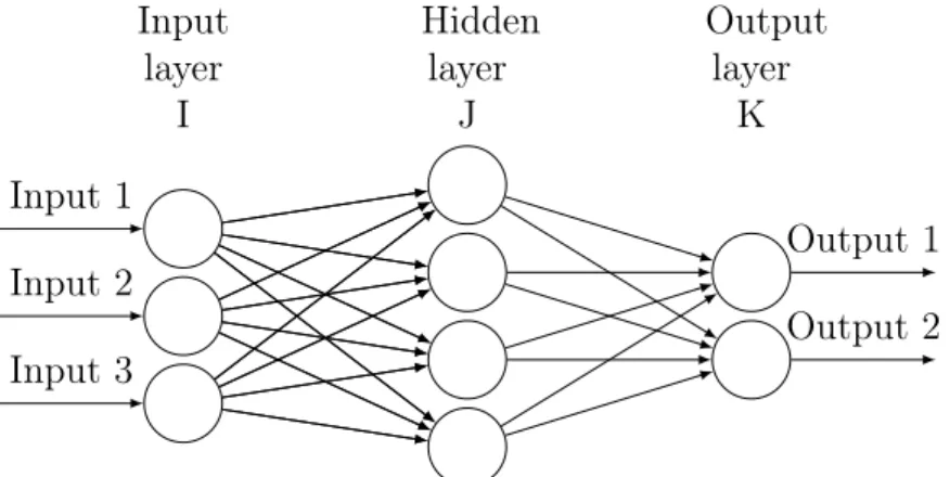
There are three major parts to MLP: the input layer, the hidden layer, and the output layer. The input layer which can also be called input neurons contains some features that can be used for training and prediction purposes. Then the features are assigned with weights (ω) and are projected into the hidden layer with a combination function as hidden neurons.

Then with another function, which is called activation function (σ), the hidden neurons are

being projected to the output layer as output neurons. The reason why MLP is categorized as supervised learning is in the sense that it requires an output as the response to complete the model.

For activation functions, Harej et al. [2017] chose Sigmoid and Hyperbolic tangent

ac-tivation functions because they fit well with the backpropagation algorithm in a way that they are continuous and diﬀerentiable:

Sigmoid function: σ(x) = 1

1 +e−x, x∈R,

Hyperbolic tangent: σ(x) = e

x₋_e−x

(41)

Input layer I Hidden layer J Output layer K Input 1 Input 2 Input 3 Output 1 Output 2

Figure 3.2: Graphical Representation of MLP with one Hidden Layer

Then in order to measure the quality of the model, mean square error (MSE) is used through the cost function:

C(ω) = $

α

(yα(ω)−tα)2, (3.15)

where ω is the weight, tα is the α-th response in the output layer, and yα is the predicted

output for the α-th response in the output layer, with yα =σ(z) = σ(ωx).

Hence the model with the smallest MSE is, in relative terms, the best model. There are other possible cost functions (e.g., the AIC or BIC criteria) that could also be considered.

Harej et al. [2017] explain how to complete the triangle, step by step, for individual claims from diﬀerent accident years; which is the method mentioned earlier, called cascading. The graphical representation of the cascading method is shown below. The steps are shown as the white colour numbers.

(a) 1 2 (b) 3 4 (c)

Figure 3.3: Graphical Representation of Cascading (Type 1)

(42)

to predict the claim reserve from the bottom left corner to the top right of the triangle by repeating Steps 1 to 4 as shown in black blocks from Figure 3.3, which are

Step 1 (Train): Train the model using the data from top left as predictors, and the data from top right as responses.

Step 2 (Predict): Use the trained model to predict the bottom right using the predictors from bottom left.

Step 3 (Train): Train the model again using the predictors from top left, and the data from top right as responses.

Step 4 (Predict): Use the trained model to predict the bottom right using the variables from bottom left.

However, Harej et al. [2017] mention a weakness using the cascading method, due to the similarity with the CL algorithm, it performs poorly on the data that contains claims with diﬀerent developments patterns.

In order to compute the parameters of the ANN model, two learning algorithms were introduced by Harej et al. [2017]; One is a standard backpropagation algorithm (BA) algo-rithm, which is a first order learning method. A simple explanation will follow.

In order to minimize the cost function (3.13), the partial diﬀerential equations ∂C(ω)

∂ω for

both output and hidden layers need to be calculated. A sigmoid function will be used here for the explanation because the diﬀerential equation is simpler to show. The diﬀerential equation of the cost function can be written as:

C′(ω) = C(ω)(1₋C(ω)). (3.16)

As shown in Figure 3.2, I, J, K are the sets of nodes from the input, hidden, and output

layers; wij are defined as the weights going from the input layer to the hidden layer, andwjk

are defined as the weights from the hidden layer to the output layer.

(43)

output layer, then we have ∂C(ω) ∂ωjk =yjδk, (3.17) where δk =yk(1−yk)(yk−tk). (3.18)

For a hidden layer,yi is the node from the input layer andyk is the node from the hidden

layer, then we have

∂C(ω) ∂ωij =yiδj, (3.19) where δj =yj(1−yj) $ k∈K δkωjk. (3.20)

If the bias term θ were considered, it would be easy to find that: ∂y

∂θ = 1. (3.21)

Hence, the backpropagation algorithm is based on the following steps:

1. Run the neural network forward with input data to get the network output tk;

2. For each output node, compute

δk =yk(1−yk)(yk−tk). (3.22)

3. For each hidden node, calculate

δj =yj(1−yj)

$

k∈K

δkωjk. (3.23)

4. Update each weight and bias as follows:

ωℓ−1,ℓ =ωℓ−1,ℓ+∆W =ωℓ−1,ℓ−ηδℓyℓ−1, (3.24)

θ =θ+∆θ =θ−ηδℓ, (3.25)

(44)

the layers (e.g j ork): if ℓ=k, then ℓ₋1 = j; if ℓ=j, then ℓ₋1 =i.

Repeating this process for some times, the optimized weight and bias can be found when the cost function is minimal. Since there might be a local minimum, the number of repetitions should not be too small. Meanwhile, a large number of repetitions can be time-consuming. Therefore, 500 epochs are the standard number of times that is used frequently.

The other learning algorithm is called scaled conjugate gradient backpropagation (SCG) algorithm (see Møller [1993]), which is a second-order learning method. A quadratic approx-imation of the cost function in the neighborhood of the point concerned was used, which can be computed by the first three elements of the Taylor expansion of the cost function,

CSCG(ω+∆ω)≈C(ω) +C′(ω)∆ω+

1 2C

′′₍_ω₎_∆_ω_. _(3.26)

In order to minimize CSCG, the critical points need to be found where

C_SCG′ (∆ω) =C′′(ω)∆ω+C′(ω) = 0. (3.27)

The final algorithm for SCG was given by Møller [1993], which has the following 9 steps: 1. Choose weight vector ω1 and scalars σ>0, λ1 >0, and λ¯1 = 0:

Set p1 =r1 =C′(ω1), k= 1 and success = true.

2. If success = true, then calculate second order information:

σk = σ |pk| , (3.28) sk = C′(ωk+σkpk)−C′(ωk) σk , (3.29) δk =pTksk. (3.30) 3. Scale sk: sk =sk+ (λk−λ¯k)pk, (3.31) δk=δk+ (λk−λ¯k)|pk|2. (3.32)

(45)

4. If δk ≤0then make the Hessian matrix positive definite: sk =sk+ (λk−2 δk |pk|2 )pk, (3.33) ¯ λk = 2(λk− δk |pk|2 ), (3.34) δk =−δk+λk|pk|2,λk= ¯λk. (3.35)

5. Calculate the step size:

µk =pTkrk, αk=

µk

δk

. (3.36)

6. Calculate the comparison parameter:

∆k =

2δ[C(ωk)−C(ωk+αkpk)]

µ2

k

. (3.37)

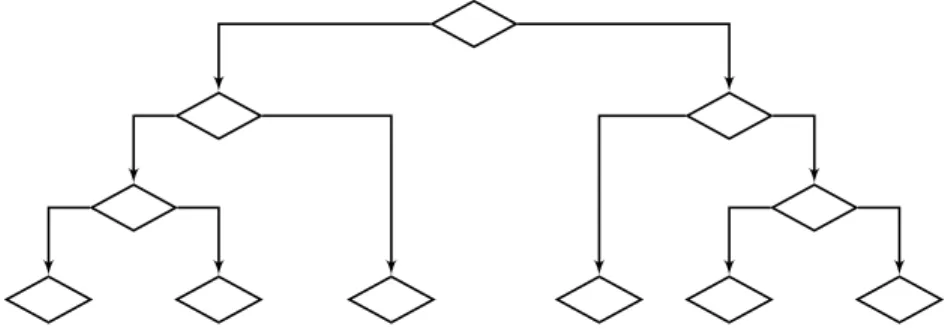
7. If ∆k ≥0, then a successful reduction in error can be attained as:

ωk+1 =ωk+αkpk, (3.38)

rk+1 =C′(ωk+1), (3.39)

λk= 0, success=true. (3.40)

7a. If k mod N = 0 then restart the algorithm: pk+1 =rk+1+βkpk,

else create a new conjugate direction:

βk= | r2 k+1−rk+1rk| µk , (3.41) pk+1 =rk+1+βkpk. (3.42)

7b. If ∆k ≥0.75then reduce the scale parameter: λk= 1₂λk,

else a reduction in error is not possible: λk = 4λk, success = false.

8. If ∆k <0.25then increase the scale parameter: λk = 4λk.

Individual Claims Reserving: Using Machine Learning Methods