Mortgage Pricing: What Have We Learned So Far?

MORTGAGE PRICING:

WHAT HAVE WE LEARNED SO FAR?

Patric H. Hendershott

Working Paper No. 1959

NATIONAL BUREAU OF ECONOMIC RESEARCH 1050 Massachusetts Avenue

Cambridge, MA 02138 June 1986

This paper -is a revision of the 1985 Presidential Address and will appear -in the AREUEA Journal, Winter 1986. _{I thank Stephen Buser} for his thoughtful insights on many of the issues discussed -in this paper and T.C. Langetieg and Robert Van Order for their perceptive comments on an earlier draft. The research reported here is _part of the NBER's research program in Financial Markets arid _Monetary Economics. Any opinions expressed are those of the author and not those of the National Bureau of Economic Research.

June 1986

Mortgage Pricing: What Have We Learned So Far?

ABSTRACT

Much progress has been achieved in the valuation of call options and interest—rate caps on default—free mortgages. The evidence suggests that the observed term structure of interest rates (the full structure, not just the end points) and a reasonable estimate of the volatility of spot rates is sufficient for pricing purposes. Knowledge of the precise nature of the interest—rate process and the exact market price of interest—rate risk, the not—well— identified determinants of the term structure, are not _{necessary for pricing.}

(The analogy to pricing stock options is striking; there, knowledge of the observed stock price —— _{and the present value of expected future dividends ——} and _{a reasonable estimate of the volatility of the stock price are sufficient} to price the option.) Moreover, the number of interest—rate state variables is also of little import, again holding the term structure and rate_volatility constant.

Pricing the mortgage default option, in contrast, is still in the

embryonic stage. The stochastic process analogous to the interest—rate process in valuing call is a house price process: if a house price declines

sufficiently, default occurs. The observed house price, the present value of expected future "dividends" (rents), and the volatility of house prices is, in principle, sufficient to value default (again note the analogy to stock price options). Unfortunately, rents are unknown, and no observable term—structure of expected future house—price inflation—rates exists from which to glean the division of expected housing returns between "dividends" and expected capital gains. Also, a series on the recent volatility of individual house prices is not readily available. Finally, measurement of the costs to defaulters and the losses of lenders/insurers when default occurs is far less straight—forward than is the case when call occurs or interest—rate caps are reached. (Here, an analogy can be drawn to the difficulties encountered in pricing the

bankruptcy risk of firms.)

Patric H. Hendershott Hagerty Hall

The Ohio State University 1775 College Road

Columbus, OH 43210

Patric H. Hendershott

Mortgage pricing is a rather dry subject. Considerably juicier is what is happening to the prices of our former mortgage—pricing colleagues. We have Ken Thygerson and Kevin Villani, the duo who used to organize AREUEA programs and write about the call option in mortgage contracts, first _{running Freddie} Mac and now buying up real—estate on the Pacific Ocean in San_{Diego. Filling} Kevin's shoes at Freddie Mac are two more of our mortgage _{pricing colleagues:} Henry Cassidy, new Vice President for Finance and former tennis pro at the Bank Board, and Mike Lea, new Chief Economist and former teacher of consumer

economics at Cornell. And let's not forget Jerry Hartzog, another dabbler at the Bank Board, who went on to be Treasurer at the FHLB of San

Francisco and, more recently, Vice President at Salomon Brothers. Of course, prices are even better for former finance professors who design options strategies for a broad range of financial instruments, as I'm sure Fischer Black, Richard Roll, Jess Yawitz and many others can tell us. But then, who really wants to be in coat and tie at seven o'clock every morning? And who wants to give up his leisurely summer on the golf course or tennis court and his quiet holiday season with his family?

Without megabucks, but with loosened tie, I now turn to the more serious subject of what we know about pricing mortgages. I'll start out with a quick review of some methodological issues and then discuss mortgages with fixed and adjustable rates. Throughout, I will be referring to default—free_mortgages. While we are learning about default —— _{how can we not help but do so when}

default rates are quadrupling? —— we are still far from being able to price default risk accurately. I will have a few words on this subject in my conclusion.

I. The Basics of Mortgage Pricing

Substantial similarity exists between fixed—rate mortgages (FRMs) and adjustable—rate mortgages (ARMs) with interest rate caps and floors. Lenders will earn below—market returns on both instruments if interest rates should rise far more sharply than expected. Moreover, rate floors on ARMs and costly call of FRMs will cause lenders to earn above—market rates of return on both instruments should interest rates decline somewhat more than expected. Because of these similarities, the fundamental determinants of the spreads between coupon rates on par—value FRMs or ARMs and the short—term market rate of interest are the same.

This mortgage coupon mark—up is largely determined by the slope of the term structure of interest rates and the longer—run volatility in short—term rates. The more upward sloping is the term structure ——

the

more lenders expect interest rates to rise and the more lenders are averse to increases in rates ——

the

_{greater will be the mark—up on fixed or capped rate loans.}

Moreover, even if the term structure is relatively flat, high long—run volatility in short rates (high short—term volatility and little mean

reversion) means a reasonable likelihood of significantly higher interest rates during some future periods. Thus the higher is long—run rate volatility, the greater is the mark—up.

-Setting

looser rate caps on ARMs and introducing ARM rate floors and/or costly call modifies the relationship between the mark—up and its determinants. The looser are the rate caps and the more costly is call or prepayment, the less the mark—up will be for a given slope of the term structure and level of long—run rate volatility. With loose caps, lenders lose less relative to

market rates when rates rise; with costly call and/or rate floors, lenders gain relative to market rates when rates decline. How much the mark—up is reduced again varies with the slope of the term structure and the long—run volatility in rates. Pricing mortgages, then, depends crucially on the

assumptions made regarding possible future interest—rate paths, as well as on the terms of the mortgage contract.

A. Modelling Interest Rates

In general, the interest—rate process is modelled in continuous time as a diffusion process about an expected drift over time. More formally, the change in the spot rate, dr, is the sum of a time drift term and a diffusion term:

a

dr =

_k(u—r)dt

+

or

_{dz, (1)}

where u is the value toward which the spot rate is reverting, with k being the speed of reversion, or5 is the standard deviation of the spot rate (a and are constants) and dz is a standardized Gauss—Weiner process (dz has

independent increments that are normally distributed with a mean of zero and variance of dt). The dependency of the standard deviation on the level of

interest rates prevents negative interest rates from occurring; an a less than unity or k greater than zero prevents rates from exploding. For a given

specification of u (such as the long—term Treasury rate) and a (usually or unity), values of k and a can be obtained by the estimation of

r

_{u_r1}

+ OE

r

_t—l r t

where is a random error and the equation standard error equals a (Brennan and Schwartz, 1982; Buser and Hendershott, 1984). The estimates researchers obtain for mortgage mark—ups will depend crucially on the assumptions made about the drift (U and k) and volatility (are) of interest rates.

The current spot rate, r, is known at any point in time that one wishes to price mortgages, but the mean—reverting value, u, is not. The natural method of choosing u is to select a value consistent with the existing term

structure of interest rates (Buser, Hendershott and Sanders, 1985). If fixed— rate mortgages are being priced, one might select the u that prices eight—year Treasuries correctly; if one—year adjustable rate mortgages are being priced, the u that prices one or two year Treasuries accurately might be chosen.

An alternative to working with this general diffusion process is to price directly off the yield curve (Crane and Lea, 1985). To illustrate, the one— period yield one period out, r1, is expressed as the forward rate implied by the term structure, y1, plus a random error, cc

r1 =

_y1

+

_cc1,

where a is again chosen to reflect the expected volatility in interest rates. For two periods in the future,

r2 =

_y2

+ _k(r1—y1) +

_cc2.

The k term allows earlier random errors to have a persistent role over time. With k =

_0,

_{strong reversion to the implied yield curve exists; assumed spot}

rates over time are those implied by the current yield curve plus the single random error:

r =

+

With

k >

_0,

t—l

r =

+ oE k'

_Eti.

(2)

That is, past errors also shift expected future spot rates from the value implied by the current yield curve.

B. Pricing Models

Using the interest—rate process given in (1) ,

with

= and a zero— arbitrage risk/return condition, one can derive [Merton (1973)]

V +

_[k

+

k

(u—r) +

aXr]V

+ C —

_rV

=

_0,

(3)

t 0 1 r rr

where V is the value function, the subcripts on V denote partial derivatives with respect to time and the spot rate, Ar½ is the market price of interest—

rate risk and C is the instantaneous cash flow on the mortgage (amortization plus interest). Solution to this equation (subject to boundary values at

extremely high and low interest rates and to the terms of the mortgage contract determining C) yields the equilibrium price path of the mortgage. By trial and error, one can compute the coupon on the mortgage necessary for the mortgage to be initially valued at par (see below for more details)

An alternative solution is obtained by using the Monte Carlo forward— solving method. One begins with the large array of possible interest rate scenarios (say k, which may be in the thousands) obtained from the yield curve as described above, each with its own probability of occurring. The present value of the mortgage payments in the kth scenerio, where

_{CASH(r +}

_{m) is the} tth anticipated cash flow (scheduled and early payments) and depends on the

coupon mark—up m over the initial spot rate, is N CASH (r + m) k ₌

to

(4)

t—l II(l+r)

j=O

The mark—up is then computed as that which will equate a weighted average of the present values in the different scenarios to par

kpk =

PAR =

v,

(5)

where the p's are the probabilities of the scenarios occurring if there is zero risk aversion (x= 0) and are the pseudo probabilities if aversion exists (Cox, Ross and Rubinstein, 1979). (Alternatively, one can calculate the present value of the mortgage payments, assuming no mark—up, for each interest rate

scenario, average these, and then compute the mark—up that will raise this present value to par.)

The forward—solving model will provide incorrect results if (1)

termination of the contract depends importantly on future values of the state-. variable ——

the

spot rate of interest in our case —— and (2) if the current value of the contract depends importantly on when the contract might be

terminated. This problem explains why the forward—solving model is popular in valuing ARMs but not FRMS. In the absence of rate floors, the call option on a short—term ARM has little value to the borrower and thus will cost the lender a negligible amount. All the borrower achieves by calling is a lower life—of— loan rate cap. A three percentage point decline in the ARM index, for example, converts what was originally a five—point life—of—loan cap to an eight—point cap. Because the gain from lowering the cap from eight to five is so small

relative to the cost of refinancing, call is unlikely. Thus a forward—solving valuation of rate caps only would lead to a minor understatement, at most, of the margin needed on short—term ARMs without floors.

As ARMs become longer term and rate floors are introduced, the instrument becomes more like a FRM and the call value grows larger relative to the _cap value. To make the point clear, consider a fixed—rate mortgage. Use of the Monte Carlo forward—solving method would probably cause one to choose the new— issue mortgage rate as the interest—rate state variable. If call is _costless, then refinancing will occur whenever the mortgage rate falls below the initial rate. However, if refinancing costs exist ——

_origination

_{fees, prepayment} penalties, or simply an upfront charge for the call option ——

difficulties

arise. Say that the mortgage rate must fall by two percentage points for call to be marginally profitable. Will call occur if the rate falls by two and a half points? Not necessarily. The borrower will gain from the _refinancing, but he gives up a valuable call option in the process (Siegel, 1984) .

If

the

borrower did not call and interest rates were to fall by another two points, the borrower could then get a full 4½ point reduction in rate ——

_which

_includes a pure gain of 2½ points over the 2 points needed to offset refinancing costs ——

in

contrast to a half point pure gain if earlier refinancing had occurred. In this case, one cannot accurately evaluate future events without knowing the likelihood of events even beyond. _{(The same problem exists in using forward—} solving models to price default risk: one cannot evaluate default

probabilities in future periods without knowing the value of the unused default option, which depends on events even beyond.)

This problem can be finessed by reversing the direction from which the problem is attacked, i.e., by starting at the end of the contract, where the call option is known to be worthless, and working backward in time. For the partial differential equation (3) , one starts with a feasible array of, say, 50 spot rates at the end of the life of the fixed—rate contract and evaluates the

known final payment at each of these rates. One then computes the contract values one period back in time for each of the same spot rates, solving the differential equation using the "implicit—difference method" (Brennan and Schwartz, 1977) and the boundary values at the interest—rate extremes.

One of the low interest rate boundary values for a callable mortgage is the remaining book value of the mortgage plus the prepayment or refinancing penalty; call or prepayment occurs when the interest rate falls sufficiently for the contract to rise to this value. Should this value be reached, it replaces the original solution value. One progresses in this way back to the initial period. The mortgage value in the initial period at the spot rate known to exist at that time is the final solution. If this value differs from par, the mortgage contract can be altered (the C in equation 3) and the

procedure repeated. (While the backward—solving can also be used in the Monte Carlo method, the calculations became exceedingly tedius. In effect, a

different PAY stream must be pre—specified for every interest rate scenario.) While the backward—solving method is ideal for fixed—rate mortgages, problems arise when it is applied to pricing different tranches of

collateralized mortgage obligations or adjustable—rate mortgages with caps because the contract cash flows on these instruments depend on the unknown path of spot rates in earlier periods (the reverse of the problem of forward—solving when termination depends on the unknown path of interest rates in later

periods). With an ARM life—of—loan rate cap, the problem is minor; only the amortization is unknown, given today's spot rate, and the valuation is

insensitive to amortization extremes (linear being the most rapid and that with the coupon at the life—of—loan cap being the least: Buser, Hendershott and Sanders, 1985) .

With

adjustment period rate caps or CMOs, neither forward nor backward solving is adequate. The solution to this dilemma is iteration

between backward and forward solving solutions. This is achieved by the introduction of a second state—variable to keep track of the sample path of interest rates (Dale—Johnson and Langetieg, 1984, and Kau et al, 1985).

A major difficulty in these pricing methods is their complexity. Not only are the models difficult for researchers to implement (setting the

boundary conditions is the most difficult task), but the output of the models is nearly impossible for users to verify. All researchers in this area must be extremely careful in documenting their work and should design experiments to check their calculations against known analytical solutions. Alternatively (or supplementarily) they might use both the differential—equation and Monte Carlo methods to price the same mortgage. Moreover, they should devote some effort to verification of the results of others. This is no trivial matter. My collaborators and I have attempted to verify the results of five studies and have been fully successful only once. I shall return to this point below.

II. Evidence on the Value of the Call Premium in FRMs

Dunn and McConnell (l98la, l981b) were the first to apply the backward— solving model to fixed—rate default—free mortgages. _{(Asay, 1978, applied the} model to value the default option in fixed—rate mortgages.) They illustrated how the methodology developed by Brennan and Schwartz (1977) for nonamortizing bonds could be applied to amortizing 30—year mortgages and showed the general implications of amortization. Buser and Hendershott (1984) examined the sensitivity of the simulated call values to the assumed parameters and valued 15—year level—payment mortgages and 30—year graduated—payment mortgages, as well as the standard 30—year level—payment mortgages. In a recent issue of AREUEA, Brennan and Schwartz (1985) ,

the

pioneers of the application of

numerical methods to the pricing of debt instruments, turned their attention to pricing FRMs. They employed their two—state interest—rate model (both the

short—term rate and the mean—reverting value are uncertain) ,

which

they contend leads to substantially more accurate pricing, to obtain realistic estimates of the call value on 30—year FRMs.

Unfortunately, the Buser and I-Iendershott paper contained an error, and we have been unable to reproduce the Brennan and Schwartz results (we did

reproduce the Dunn—McConnell results) . _Thus, my- collaborators and I have resimulated call values on par value 30—year FRM5. Realistic values of the call premium were obtained for both the 1970s and the early l980s for different slopes of the yield curve. For the l970s, the spread over the spot rate at time of issue ranged from 90 basis points (negatively sloped yield curve) to 350 basis points (steeply positively sloped yield curve) -

For

the 1980s, the range was 20 to 30 percent greater. The higher values in the 1980s are due to a larger volatility in interest rates, although this is partially offset by a faster reversion of the spot rate to its mean—reverting value.

The call premium on FRMs is usually reported as the difference between the mortgage coupon and the coupon on a noncallable mortgage with the same amortization schedule as the callable mortgage, not the difference between the mortgage coupon and the spot rate. In the l980s, the spread over the

noncallable mortgage coupon is roughly 275 basis points when the yield curve is downward sloping (and call is likely), but just under 100 basis points when the yield curve is steeply upward sloping (and call is unlikely). In the 1970s, call premia were less; about 200 basis points for the negatively—sloped yield curve and only 50 to 75 basis points for the steeply upward—sloping yield curve. (Hall's estimates, 1985, are generally consistent with these values, but precise comparisons are not possible because he did not compute his estimates for specific yield curves.)

These calculations suggest an enormous swing in the call premia over the past decade. In 1976—77 and again 1983—84, a 250 basis point positively sloped yield curve prevailed. In contrast, in late 1979—early 1980 and again in much

of

1981 a negative slope of over 100 basis points existed. Thus the call premia, by our calculations, should have risen from 60 basis points in 1976—77 to over 250 basis points in the early 1980s and then declined to under 100 basis points. Observed spreads between par—value GNMA coupons and comparable maturity portfolios of noncallable Treasuries have moved in roughly this manner

(Hendershott, Shilling and Villani, 1983)

Cassidy (1983) and Dietrich et al (1983) estimated the value of a partial offset to the call option ——

_the

_{forced prepayment of the mortgage when the} house is sold. Cassidy, using a forward pricing Monte Carlo simulation,

computed the option to be worth 30 to 80 basis points, i.e., elimination of the due—on—sale option of lenders would raise coupons rates on nonassumable

mortgages by that amount. Dietrich et al, solving the partial differential equation backwards, reported somewhat higher estimates, 50 to 100 basis points.

Intuitively, these values seem too high. First, unlike the call option, the due—of—sale option is likely to be exercised relatively late in the life of the mortgage and thus is worth relatively less in present value terms.

(Hendershott, Hu and Villani provide an example in which the value of

assumability is worth only a quarter as much as the value of call, 1983, _pp 139—141.) Second, due—on—sale can be exercised only if households

actually sell their houses and many will expressly avoid selling in order to maintain a far below—market mortgage (Hendershott and Hu, 1982). Thus one might expect due of sale to be worth not more than a fifth as much as the call _{option. With} call being worth 100 to 250 basis points, due—on—sale should be worth 20 to 50 basis points at most.

A final methodological point. All of the cited studies using the partial differential equation method employed a single—state variable except Brennan and Schwartz (and Asay) . The latter argue that a second state—variable is necessary for pricing default—free contingent claims. However, our results

(Buser, Hendershott and Sanders, 1986) show that the second—state variable has a negligible impact on mortgage prices, again as long as the term structure and interest rate volatility are held constant.

III. ARM Margins

Given the only recent popularity of ARMs, the volume of research of their pricing has been enormous. The published work, and it is only the tip of the iceburg, includes both forward—pricing Monte Carlo analyses by Asay (1984) and Lea (1985) and backward—pricing calculations by Buser, Hendershott and Sanders

(1985) and Kau et al (1985). Not only do the studies use different pricing methods, but they assume different interest—rate processes and variances,

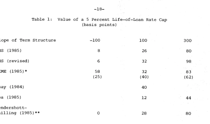
different slopes of the term structure, and even slightly different instruments (one—month versus one year, callable versus noncallable) . Thus comparisons of results is difficult. Nonetheless, I have "reproduced" in Table 1 the implied values of a five percent life—of—loan rate cap for different slopes of the term structure (approximately the same across the studies) as a means of

illustrating the general nature of the results. (The slope refers to the spread between yields on par—value 30—year and 3—month Treasuries.)

In spite of the substantial differences in assumed interest—rate

processes, the two BHS studies compute roughly the same cap values: under 10 basis points with the negatively—sloped yield curve and thus expectations of declining future rates, about a third of a percentage point for the normal upward sloping yield curve, and three—quarters to a full percentage point with a steeply upward sloping yield curve and expectations of sharply higher future rates. This illustrates a general point, namely that knowing the yield curve and the approximate variance of spot rates is sufficient to price alternative mortgage features. The Kau et al values are roughly comparable for upward—

sloping yield curves, but their cap value for a negatively sloped yield curve (rates expected to decline) is sharply higher, nearly double their estimate

when the yield curve has the normal gently rising upward slope (this anomoly exists for all the ARM contracts they analyze). We have attempted,

unsuccessfully, to reproduce their results; values (listed in parentheses beneath their values in the Table) based on our interpretation of their parameterization show the expected pattern of increasing cap values as

expectations of falling interest rates switch to expectations of rising rates. The forward—pricing Monte—Carlo analyses are not available for all the different term structures. For the normal yield curve, Asay's 40 basis point estimate is roughly comparable to the BHS estimates, and Lea's estimates, like those of BHS, roughly triple as the yield curve rotates from normal to steeply upward sloping. However, Lea's estimates are only about half as large as BHS, possibly reflecting a lower assumed variance (Lea does not state his assumed value) . The _{last row in the table reports the minimum, average, and maximum} margins lenders would have needed to have earned the market rate of return on hypothetical ARMs with a 5 percentage point life—of—loan cap issued in the years 1970 through 1976. Interestingly, these ex post values correspond roughly to the ex ante values for the negative, normal, and steeply positive term structures.

IV. Conclusions

Much progress has been achieved in the valuation of call options and interest—rate caps on default—free mortgages. The evidence suggests that the observed term structure of interest rates (the full structure, not just the end points) and a reasonable estimate of the volatility of spot rates is sufficient for pricing purposes. Knowledge of the precise nature of the interest—rate process and the exact market price of interest—rate risk, the not—well—

identified determinants of the term structure, are not _{necessary for pricing.} (The analogy to pricing stock options is striking; there, knowledge of the observed stock price —— and the present value of expected future dividends ——

sufficient to price the option.) Moreover, the number of interest—rate state variables is also of little import, again holding the term structure and rate volatility constant.

Pricing the mortgage default option, in contrast, is still in the

embryonic stage. While our understanding of default has increased greatly in recent years (see Van Order, 1985, for a discussion and references) ,

our

pricing has not progressed far beyond Asay's original piece. The stochastic process analogous to the interest—rate process in valuing call is a house price process: if a house price declines sufficiently, default occurs. The observed house price, the present value of expected future "dividends" (rents), and the volatility of house prices is, in principle, sufficient to value default (again note the analogy to stock price options) .

Unfortunately,

rents are unknown, and no observable term—structure of expected future house—price inflation—rates exists from which to glean the division of expected housing returns between

"dividends" and expected capital gains. Also, a series on the recent volatility of individual house prices is not readily available. Finally, measurement of the costs to defaulters and the losses of lenders/insurers when default occurs is far less straight—forward than is the case when call occurs or interest—rate caps are reached. (Here, an analogy can be drawn to the difficulties encountered in pricing the bankruptcy risk of firms.)

REFERENCES

Asay, M. "The Rational Pricing of Mortgage Contracts." Ph.D. Dissertation, University of Southern California, Los Angeles, 1978.

_____

"Pricing

and Analysis of Common ARM

_Products,"

_{Mortgage Banking,} December 1984.

Brennan, M.J. and Schwartz, E.S. "Savings Bonds, Retractable Bonds and Callable Bonds," Journal of Financial Economics, August 1977.

____

"An Equilibrium Model of Bond Pricing and a Test of Market Efficiency," Journal of Financial and Quantitative Analysis 17, 1982.

_____

"Determinants

of GNMA Mortgage Prices," AREUEA Journal, Fall 1985.

Buser, S.A. and Hendershott, P.H. "Pricing Default—Free Fixed—Rate

Mortgages," Housing Finance Review, October 1984.

Buser, S.A., Hendershott, P.H. and Sanders, A.B. "Pricing Life of Loan Rate Caps on Default—Free Adjustable—Rate Mortgages," AREUEA Journal, Fall 1985.

,"The Term Structure and Mortgage Prices," NBER Working _{Paper, 1986.}

Cassidy, H.J. "Monte Carlo Simulation Estimates of the Expected Value of the Due—on—Sale Clause in Home Mortgages," Housing Finance Review, _{January 1983.}

Cox, J.C., Ross, S.A. and Rubinstein, M. "Option Pricing: A

Simplified Approach," Journal of Financial Economics, September 1979.

Crane, R.C. and Lea, M.J. "Pricing Rate—Capped ARMs," Secondary Mortgage Markets, Summer 1985.

Cunningham, D. and Hendershott, P.H. "Pricing FHA Mortgage Default Insurance," Housing Finance Review, October 1984.

Dale—Johnson, D. and Langetieg, T. "The Pricing of Collateralized Mortgage Obligations," presented at Midyear AREUEA meetings, 1984 (revision to be presented at AFA/AREUEA 1986 annual meetings).

Dietrich, J.K., Langetieg, T.C., Dale—Johnson, D. and Campbell, T.S. "The Economic Effects of Due—on—Sale Clause Invalidation," Housing Finance Review, January 1983.

Dunn, K.B. and McConnell, J.J. "A Comparison of Alternative Models for Pricing GNMA Mortgage—Backed Securities," Journal of Finance 36, 1981.

_____

"Valuation

of GNMA Mortgage—Backed Securites," Journal of Finance 36, 1981.

Hall, A. "Valuing the Mortgage Borrower's Prepayment Option," AREtJEA Journal, Fall 1985.

Hendershott, P.H. and Hu, S. "Accelerating Inflation and Nonassumable Fixed— Rate Mortgages: Effects on Consumer Choice and Welfare," Public Finance Quarterly, April 1982.

Hendershott, P.H., Hu, S. and Villani, K.E. "The Economics of Mortgage

Terminations: Implications for Mortgage Lenders and Mortgage Terms," Housing Finance Review, April 1983.

Hendershott, P.H. and Shilling, J.D. "Valuing ARM Rate Caps: Implications of 1970—84 Interest Rate Behavior," AREUEA Journal, Fall 1985.

Hendershott, P.H., Shilling, J.D. and Villani, K.E. "Measurement of Spreads Between Yields on Various Mortgage Contracts and Treasury Securities," AREUEA Journal, Winter 1984.

Kau, J.B., Keenan, D.C., Muller III, W.J. and Epperson, J.P. "Rational Pricing of Adjustable Rate Mortgages," AREUEA Journal, Fall 1985.

Lea, M. "Rational ARM Pricing and Design" in Solving the Mortgage Menu Problem, Proceedings of the Tenth Annual Conference of the Federal Home Loan Bank of San Francisco, 1985.

Merton, B.C. "An Intertemporal Capital Asset Pricing Model," Econometrica 41(5), 1973.

Siegel, J.J. "The Mortgage Refinancing Decision," Housing Finance Review, January 1984.

Van Order, R. "User Fees and Mortgage Markets," paper presented at AFA/AREUEA annual meetings, December 1985.

Table 1: Value of a 5 Percent Life—of—Loan Rate Cap (basis points)

Slope of Term Structure —100 100 300

BHS (1985) 8 26 80 BHS (revised) 6 32 98 KKME (1985)* 58 32 83 (25) (40) (62) Asay (1984) 40 Lea (1985) 12 44 Hendershott-Shilling (1985)** 0 28 80

*The numbers in parenthesis are an attempt to reproduce the KKNE results. The specific term structures computed for these three points are —82, 51 and 187 basis points.

**These values correspond to the minimum, average, and maximum margins that would have been needed for lenders to have earned a market rate—of—return on hypothetical ARNs with a 5 percentage point life—of—loan cap issued in the years 1970 through 1976.