AN EXAMINATION OF DIFFERENCES IN FINANCIAL PERFORMANCE AMONG AGE COHORTS
by
GABRIEL T. WEEDEN
B.S., Kansas State University, 2006
A THESIS
submitted in partial fulfillment of the requirements for the degree
MASTER OF SCIENCE
Department of Agricultural Economics College of Agricultural
KANSAS STATE UNIVERSITY Manhattan, Kansas
2008
Approved by: Major Professor Dr. Langemeier
Copyright
GABRIEL T. WEEDENAbstract
The overall objective of this study was to examine the relative efficiency of farmers in various age groups. Nine Hundred sixty-four sole proprietors, who were members of the Kansas Farm Management Association (KFMA) with continuous data from 2002-2006, were split up into four groups based on age. Comparing the fourth age group (over 65 years of age) to the first age group (under or equal to 45 years of age) was of primary importance in this study.
Comparisons were made utilizing variables pertaining to farm size and tenure, specialization, efficiency, liquidity, and solvency.
In this study, there are four age groups; under or equal to 45 years, 46 to 55 years, 56 to 65 years, and greater than 65 years old. T-tests were used to compare variables among age groups. Nineteen variables were statistically different between age groups one and four. The fourth age group performed poorly in terms of cost efficiency. Based on the results, the fourth age group had a difficult time covering unpaid labor and capital expenses. Discriminant analysis was used to determine which variables discriminate the most between age groups. The top three variables in this discriminant analysis were the asset turnover ratio, the economic total expense ratio, and percent acres owned. The top three variables in the discriminant analysis involving groups one and four were the debt to asset ratio, asset turnover ratio, and net farm income.
iv
Table of Contents
List of Tables ... vi Acknowledgements ... vii CHAPTER 1 - Introduction ... 1 1.1. Introduction ... 1 1.2. Statement of Objectives ... 2CHAPTER 2 - Literature Review ... 4
2.1. Farm Planning ... 4
2.2. Empirical Analysis of Age Cohorts ... 7
CHAPTER 3 - Methodology ... 14
3.1. Age Groups ... 14
3.2. Farm Characteristics ... 15
3.2.1. Farm Size and Tenure ... 15
3.2.2. Specialization ... 18
3.2.3. Efficiency Ratios ... 19
3.2.4. Liquidity / Solvency Ratios ... 21
3.3. Statistical Analysis ... 21
CHAPTER 4 - Data ... 23
4.1. Farm Size and Tenure ... 23
4.2 Specialization ... 26
4.3 Efficiency Ratios ... 27
4.4 Liquidity and Solvency ... 29
CHAPTER 5 - Results ... 31
5.1 T-Test Results ... 31
5.1.1 Farm Size and Tenure ... 36
5.1.2 Specialization ... 37
5.1.3 Efficiency Ratios ... 39
5.1.4 Liquidity and Solvency ... 42
v
CHAPTER 6 - Conclusions ... 47
6.1. Summary ... 47
6.2. Limitations ... 50
vi
List of Tables
Table 3.1. Definitions of Farm Characteristics, Efficiency, Liquidity, and Solvency Ratios. ... 16
Table 4.1. Means and Standard Deviations of all Farmers. ... 24
Table 5.1. P-Values of Group Comparisons. ... 32
Table 5.2. Variable Differences Among Age Groups... 34
Table 5.3. Discriminant Analysis Results - All Groups... 43
Table 5.4. Discriminant Analysis Results – Groups One and Four. ... 46
Table 5.5. Discriminant Analysis Results – Groups Two and Four. ... 46
vii
Acknowledgements
I would first like to thank my Major Professor, Dr. Michael Langemeier for his time, guidance, and insight on this project. Dr. Langemeier has become a great mentor and friend, I have especially enjoyed my time working with him. I would also like to thank my other two committee members Dr. Rodney Jones and Dr. Terry Kastens. Most of all, I would like to thank my parents and siblings for their guidance and support throughout this project. Last but not least, I would like to thank my girlfriend for always being there and believing in me.
1
CHAPTER 1 - Introduction
1.1. Introduction
Farmers are faced with many decisions on how they will go about retirement. Because of physical or health conditions, or desire to “slow down” before retirement, many older farmers begin to downsize their operations. Whether the farmer cuts back on a livestock operation or rents less land, the farmer may experience a decrease in efficiency. Previous research that examines differences in efficiency across age groups is sparse.
The 2002 Census of Agriculture for Kansas contains data from operators who indicated that their major occupation is farming. The Census split the operator‟s age into six different groups: less than 25 years, 25 to 34 years, 35 to 44 years, 45 to 54 years, 55 to 64 years, and over 65 years old. Operators under 25 years of age make up less than one percent of total farm
operators in Kansas. Operators 25 to 34 make up 5.5%, operators 35 to 44 make up 14.3%, operators 45 to 54 make up 22.9%, operators 55 to 64 make up 20.1%, and operators over 64 make up 36.4% of total farm operators in Kansas (2002 Census). The principal farm operator‟s average age increased from 53.2 in 1992 to 56.0 years old in 2002 (USDA).
The Kansas Farm Management Association (KFMA) has different age groupings than the Census of Agriculture. KFMA has nine different age groups (the percent of farms in each group is in parentheses): under 36 years (5.4%), 36 to 40 years (5.4%), 41 to 45 years (8.1%), 46 to 50 years (13.8%), 51 to 55 years (18.2%), 56 to 60 years (14.1%), 61 to 65 years (12.8%), 66 to 70 years (9.0%), and greater than 70 years old (13.4%). The two largest age groups, 51 to 55 years and 56 to 60 years, make up nearly one-third of the KFMA farms.
2
According to the 2006 KFMA‟s Annual ProfitLink Summary (Langemeier and Herbel, 2007) the age group under 36 had the highest net farm income at $58,612. Farmers with the lowest net farm income ($36,273) were in the age group over 70 years. Farmers under age 36 also had the highest average profit margins, return on assets (ROA), and return on equity (ROE). The age group over 70 had the lowest profit margin and ROA. The age group 56 to 60 had the lowest ROE.
1.2. Statement of Objectives
The objective of this thesis is to examine the relative efficiency of farmers across various age groups. Comparing sole proprietors of downsizing farms to sole proprietors of growing farms is of primary interest for this study.
Data used in this analysis comes from the Kansas Farm Management Association (KFMA). A data set obtained from KFMA containing 964 farms with continuous and usable data from 2002 to 2006 will be analyzed in this study.
Age groups are defined differently in this study than they were in the Census or KFMA. In this study, there will be four age groups; under or equal to 45 years, 46 to 55 years, 56 to 65 years, and greater than 65 years old.
When comparing differences among age groups, five variables pertaining to farm size and tenure will be used. These variables are value of farm production, total acres, percent acres owned, net farm income, and total assets. The percent of income derived from specific crop and livestock also will be compared among age cohorts. There are 14 variables used to compare efficiency; labor efficiency, purchased inputs efficiency, capital efficiency, profit margin, return on assets, return on assets with capital gains, return on equity, return on equity with capital gains, asset turnover ratio, value of farm production per worker, total expense ratio, adjusted total
3
expense ratio, economic total expense ratio, and economic total expense with capital gains. The current ratio and the debt to asset ratio will also be compared among age categories. These ratios will be will be defined in Chapter 3.
4
CHAPTER 2 - Literature Review
2.1. Farm Planning
This chapter will summarize literature pertaining to farm planning and empirical analysis of age cohorts. Previous literature will be used to help develop the methodology discussed in the next chapter.
In this day and age a successful farmer must be motivated, have certain resources (land, labor, capital), develop a long-range plan, and work toward its implementation. Even though there are no legal requirements, educational requirements, or licenses to become a farmer, substantial barriers to entry still exist. Major barriers include large amounts of land, machinery, capital, and excellent managerial skills. Capital requirements keep rising as labor requirements fall. As late as 1940, labor still accounted for over half of the resources used in farming. Today, labor accounts for less then 20% of resources used (Thomas, 2002). With farms becoming larger and more complex, increased emphasis is being placed on management. A high degree of
technical knowledge and marketing skills, both on the input and output sides of the business, are important.
Most businesses, including farming, have a life cycle of three stages: (1) entry or establishment, (2) growth and survival, and (3) exit or disinvestment. Sole proprietorships and family farms are excellent examples of how the life cycle changes.
During the entry stage, prospective farmers look at the opportunities of farming versus other careers. The “agricultural career ladder” is a progression through the life cycle.
5
basic set of machinery or livestock, rent land or buildings, establish part ownership of farmed land, and become the principal operator of the farm business (Olson, 2003). Keys to a successful entry are excellent managerial skills, land tenure, and capital.
During the growth stage, farmers acquire more resources to expand the base of the business and implement new strategies to correct inefficiencies. Risk management is also important to avoid the unpredictable changes in the market, weather, and disease.
During the exit stage, farmers retire and pass resources and responsibilities on to the next generation or neighboring farmers. The retiree may retain assets such as land, but may sell or transfer ownership of other resources such as machinery.
There are many factors that need to be considered when retiring. Farmers like, small business owners, have a lot of freedom when it comes to retiring. They can make a full exit out of farming or gradually retire. Having a large amount of freedom, many farmers give very little thought to retirement until they are ready to retire. Due to lack of retirement planning, many farmers never retire because they do not want to, they do not know what else to do with their free time, or they cannot afford to. Retirement lifestyle is determined or influenced by one‟s
financial situation, personal desires, spouse‟s desires, the future of the farm business, outside forces such as economic conditions, and government programs and regulations.
There are five major factors that affect one‟s retirement plans: (1) pre-retirement lifestyle, (2) present health and financial situation, (3) future of the farm business, (4) goals and desires of one‟s spouse and/or other affected parties, and (5) outside forces (Thomas, 2003). When dealing with pre-retirement lifestyle one should avoid drastic changes in early years of retirement to make the latter years less stressful. Present health and financial situation can affect the timing and degree of retirement. There are many questions to be asked about the future of the farm
6
business. Who will be taking over the farm? Will a family member be taking over the farm? Is it too risky to bring a family member into the business? Will there be an estate transfer at retirement? Should assets be liquidated or rented out? Before retirement one needs to discuss the topic with his/her spouse and other affected parties to make sure goals and desires are not conflicting. Outside forces can affect financial aspects of one‟s retirement.
Is farming a way of life or a business? Blank (2005) argues that it is a way of life for small farmers and a business for large scale commercial farms. More Americans are pursuing a rural lifestyle and migrating out of the cities. Over the past decade, farms with less than $10,000 in annual sales have increased. Smaller “hobby farms” tend to be located near urban areas while larger commercial farms tend to be located in rural areas. Farmland around urban areas is increasing because of non-ag influences such as urban development.
On average, capital gains have increased owner-operators‟ wealth relatively more than profits, from farming (Blank, 2005). This indicates that some owner-operators may be “real estate investment” farms choosing to capture capital gains rather than trying to be “real” farms and live off of production income. Knowledge of increased capital gains through real estate demonstrates farmers have a desire to build wealth just as businesses do. Historically, about 75% of farm assets are represented by land values. Capital gains primarily come from farm real estate. The distribution of capital gains is more likely to be heavily weighted toward the small “hobby farms,” located near urban areas, rather than large commercial farms, located in rural areas. The 2002 Census of Agriculture reports that 53.3% of all farms generate a net loss for the year. Average household earnings from farming activities in 2002 was $3,473 (USDA). The average off-farm income for farm households in 2002 was $62,285. Small farms tend to average
7
more off-farm income than larger farms. The U.S. average household income in 2002 was $52,852, which indicates farm households may be building wealth faster than other Americans.
2.2. Empirical Analysis of Age Cohorts
Sumner and Leiby (1987) conducted a study on grade A dairies in 11 southern states in 1983. A questionnaire was sent out with a purpose of gathering current herd size, annual milk production, quantities of inputs, technology used, age, schooling, experience of operators, herd size in 1977, and projected herd size for 1987. This study emphasized the relationship of human capital of the operator to the cross sectional size and growth patterns.
The average age cohort was between 51 and 55 and average herd size peaked in 1982 with 138 cows. After age 30, the average schooling cohort declined for each successive age cohort. There was a big difference in the debt to equity ratio for those under the age of 35 (roughly 45%) compared to those over the age of 55 (roughly 80%). Size of the dairy herd significantly increased with a college degree. Herd size increased with age and experience until around age 55, then each additional year decreased herd size by 1%. For each additional year of schooling, herd size increased by 3%. Higher amounts of human capital increased herd size. Management was also very important for herd size growth, especially during 1977 to 1982, when herd size increased by 9%. Results from this study showed that human capital, education, and management were essential for dairy herd growth. However, the herd growth rate was actually lower for the more experienced farms.
With an understanding of the farm life cycle one can evaluate the possible inefficiencies of the entry and exit stages of farming. This has become a major issue for agriculture, with concerns over declining farm entry and legislation aimed at helping prospective farmers. Gale (1994) conducted a longitudinal study that surveyed individual farms from three Midwestern
8
states and examined the correlation of age with farm size and growth, tenancy, entry, and exit. Results showed that new and younger farmers faced financial barriers that limited the size of the farms they operated.
Longitudinal data for individual farms were gathered from the U.S. Censuses of Agriculture in 1978, 1982, 1987. The data were narrowed down by choosing sole proprietors whose main occupation was listed as farming, and were classified in the proper federal Standard Industrial Classification (SIC) category in at least one of the three censuses. By focusing only on sole proprietors, one can find the principal operator‟s age, and total acres rented and owned, which was used to measure farm size.
Multiple regressions were run to determine any correlation between farmer age and experience on farm size and growth. There were more farmers exiting the business than entering for each census period. The mean age of entrants was in the high 30s while mean age of exits was in the low 50s. Results showed that farm size increases with age at a decreasing rate, it tended to peak when the farmer was between 40 and 50 years old, and declined thereafter. Age coefficients indicated that older farmers have larger farms than younger farmers up to about age 40. The average farm for a 20-year-old was half the size of that of a 45-year-old, and the average size at 65-year-old was two-thirds the size of that of a 45-year-old. The relationship of tenancy to age and entry status showed that financial constraints limited younger farmers. Renting was more common for younger farmers than for farmers over age 45. New entrants, because of financial barriers, may be constrained to operate a farm below the most efficient size. Older farmers may be slowing down and therefore, may not be as efficient as the middle aged farmers.
9
Tauer (1995) conducted a study that estimated farmer productivity by age. A major assumption made was that technology within a region is consistent across all age groups. However, various age groups may exhibit different efficiencies in utilizing that technology. Efficiencies were estimated for 10 production regions divided using USDA information. Age cohorts followed the 1987 Census age intervals, which created six age groups. Productivity was estimated with data gathered from 44 states.
Evidence showed that farmers over the age of 65 had higher sales-to-expenditure ratios than any other age group. This means they are slowly liquidating and starting to exit farming. The age coefficient was positive and statistically different than zero in all 10 regions. Results showed that farmer productivity generally increases with age, peaks, and then decreases with age. Not all regions showed symmetry between age and productivity. The Corn Belt Region did not become more efficient with age, but did become less efficient after mid-life. Results indicate that middle-aged farmers (35-44 years) were 10 to 20 percent more productive than the youngest (under 25 years) and oldest (over 65 years) age groups.
Purdy, Langemeier, and Featherstone (1997) examined the financial performance of 320 Kansas farms and showed the impact of risk and specialization on mean financial performance. The impact of specialization and risk on mean financial performance depended primarily on economies of size and economies of scope. Seven variables were used to examine differences in financial performance among farms: risk, age of operator, percentage of acres owned, financial efficiency, leverage, specialization, and farm size.
The variables with the most significant impact on financial performance were risk, age of operator, financial efficiency, and farm size. Age of operator was negatively related to average return on equity, thus decreasing financial performance. Age of operator had a more significant
10
impact on financial performance than percentage of acres owned. The study also looked at the effects of specializing in swine, dairy, beef, or crop production. Results showed that specializing in swine, dairy, or crop production increased financial performance, but financial performance was lower for those that specialized in beef production. Farms specializing in crop production had the most variability in financial performance. Farms with both livestock (swine, dairy, or beef production) and crop production tended to have less variability in financial performance, suggesting that this mix reduces risk through diversification.
According to Weiss (1999), farm growth and survival are significantly influenced by operator age, schooling, gender, size of farm family, off farm employment, and initial farm size. This study showed that there was a nonlinear relationship between farmer‟s age and probability of survival. There was a positive probability of survival for young farmers up to the age of 51 where it then became negative. Life-cycle effects on farm growth were significant for full-time farms but were irrelevant for part-time farms. For full-time farmers, agriculture-specific
schooling played a major role in survival and farm growth. Higher levels of schooling increased the probability of survival by 1.57% and raised farm growth by 1.69%. The level of schooling for part-time farmers was insignificantly related to firm growth and survival.
Evidence showed that gender plays an important role in farm growth rates. Farms operated by a female operator posted a 4.39% lower growth rate than farms operated by males, other things being equal. Another variable that affected survival and growth was farm family size. If the principal operator was married the probability of survival increased 4.64% and the growth rate increased 5.26%. Family members living on the farm between ages six and fifteen increased the probability of survival by 1.90% and increased the growth rate by 2.39%.
11
Results from the study by Weiss (1999) showed that small farms grew faster than larger ones. The study supported the “disappearing middle” which has direct correlation with off-farm employment status. Farms were either growing and moving to the next class size higher or taking off-farm jobs and reducing farm size. Full-time and part-time farms were causing structural change in the farm sector.
Studies have shown that productivity exhibits a life-cycle pattern. This is significant because agricultural productivity may decrease as the U.S. farm population ages. Life-cycle changes are critical in succession planning for family farms. Tauer and Lordkipanidze (2000) examined efficiency, technology use, and operator age. Productivity is the product of efficiency and technology indices. Nonparametric linear programming was used to compute Malmquist productivity indices. Productivity is measured by the ratio of outputs to inputs. In a paper by Tauer and Lordkipanidze (2000) a firm is defined as farmers in a specific age group.
Data for the Tauer and Lordkipanidze (2000) study were attained from the 1992 Census of Agriculture where farmers are split into six different age groups. Data were gathered from all 50 states, but for various reasons five states were excluded. The study excluded farmers over 65 years of age from the analysis because they are liquidating assets, which results in larger outputs relative to inputs. The states were split up into four regions; Northeast, Midwest, West,
Southeast. Within each state the productivity and technology index of the age group “under 25 years” was used as the base group for that state.
Results showed that a farmer‟s productivity increases slightly with age and then
decreases. However, there is significant variation by state. Productivity peaks at age 25-34 in the Midwest, 35-44 in both the West and Southeast, and 45-54 in the Northeast region. In Kansas, productivity peaks at age 25 to 34 with minimal decreases in productivity until age 54. After age
12
55, drops in productivity are more significant. Efficiency patterns are consistent with the belief that as farmers age they become more efficient. In the Midwest, efficiency change over age is minimal. The majority of change in productivity was due to technology use by age rather than efficiency change.
Briggeman, et al. (2007) conducted a study based on farm household typology and the implications dealing with agricultural policy. The authors argue that the U.S. farm household has been changing over the past few decades, and a new classification system is needed for agricultural policy. In the past, the Economic Research Service (ERS) typically classified farms based on size, (e.g., gross farm sales). This classification method is one-dimensional and does not capture the increasing heterogeneity of farm households in terms of sources of income, wealth, borrowing, saving and consumption behavior, and financial/business structure. The farm household‟s resource allocation decisions are the main foundation for this new classification system. A dynamic farm household utility model motivates the decisions of the operator and spouse to allocate farm household labor and investment, consumption, and credit. A new typology system was developed using cluster analysis and household decision variables.
Cluster analysis is a method used to split data into groups that are homogenous within group but are heterogeneous across groups. Results from the cluster analysis recognized a set of six mutually exclusive groups. These groups represent a new way to capture the heterogeneity of today‟s farm household in the U.S. The six groups are called single income ruralpolitan, double income ruralpolitan, active seniors, farm operator with spouse working off farm, traditional farms, and commercial farms.
Single income ruralpolitan comprised 22.3% of the overall sample. This group is distinguished by the primary worker (operator) having a full time job off the farm. This group
13
has more non-farm assets than farm assets. Labor is primarily allocated off the farm. The second group is double income ruralpolitan, which represents 23.5% of the sample. This group contains both the primary operator and spouse working off the farm. Double income ruralpolitan also had the highest household expenditures.
Active seniors made up the third group and represented 24.4% of the sample. In this group the operator primarily works on the farm, they have the lowest debt-to-asset ratio and consumption, they have unearned off-farm income and are the oldest age group. The fourth group is called farm operator with spouse working off farm which represents 12.3% of the sample. This group is comprised of the primary operator working full time on the farm and the spouse working full time off the farm.
The fifth group is traditional farms, and represents 9.0% of the sample. This group is distinguished by both operator and spouse spending a significant amount of time working on the farm. Lastly, the sixth group is commercial farms and it makes up 8.5% of the sample. This group has the operator primarily working on the farm and the spouse having a significantly smaller role in activities compared to the traditional group. The authors argue that their typology can be used to assess the impacts of government payments relative to how US farm households allocate their resources and not by farm sales.
14
CHAPTER 3 - Methodology
3.1. Age Groups
This chapter will summarize the methodology pertaining to age groups, farm
characteristics, and statistical analysis. Age groups and variables of interest are defined in detail and statistical methods are explained.
Kansas Farm Management Association (KFMA) data pertaining to sole proprietors throughout Kansas over a five year period from 2002 to 2006 were used in this study. Kansas farmers were split into three regions west, central, and east with respective percents of 14.9%, 36.9%, and 48.1%. By using KFMA data, this study will be analyzing sole proprietors because it is the most common form of business for farmers and ranchers. Also, by using sole proprietors, information such as the principal operator‟s age is known, which is highly important in this study. Partnerships and corporations are not used because of the unknown age of all of the operators or managers of the farm.
Farming follows a normal life-cycle of entry, growth, and exit. With the large generation of Baby Boomers nearing retirement age, likewise a large group of farmers are nearing the exit stage. For this study, farmers are split up into four age groups: under or equal to 45 years, 46 to 55 years, 56 to 65 years, and greater than 65 years old. The age breakdowns follow the Census of Agriculture age breakdowns except that in this study the first three Census groups are
combined into one group. This is done because of the lack of farmers participating in the KFMA program that are under age 45. The age group greater than 65 is the main focus of this study. All groups are compared to each other based on variables of interest (defined in section 3.2). For
15
example, group one is compared to group two, three, and four while group two is compared to group one, three and four, and so on. There are six total comparisons between the four age groups.
3.2. Farm Characteristics
Throughout this section numerous farm characteristics will be described dealing with farm size and tenure, specialization, efficiency, solvency, and liquidity ratios. These
characteristics are important for determining profitability and efficiency.
3.2.1. Farm Size and Tenure
In this section value of farm production, farm size, percent acres owned, net farm income, and total assets will be discussed. Since the fourth age group is the main focus, all expectations are in reference to the fourth age group, farmers over 65 years. Definitions of farm size and tenure are provided in Table 3.1.
USDA has a farm classification system developed by the Economic Research Service (ERS). The ERS focuses on family farms and categorizes them into four groups. The first group is limited resource or low-sale farms with gross sales less than $100,000. The second group is medium-sale farms with gross sales between $100,000 and $249,999. The third group is large family farms with gross sales between $250,000 and $499,999. Finally, the fourth group is the very large family farms with gross sales greater than $500,000. In this study, value of farm production is used instead of gross sales to define farm size categories.
The first variable of interest is Value of Farm Production (VFP), which is a value added measurement and can be used to measure farm size. The fourth age group is expected to have a smaller VFP.
16
Table 3.1. Definitions of Farm Characteristics, Efficiency, Liquidity and Solvency Ratios.
Farm Size and Tenure
Value of Farm Production
Total Acres
Percent Acres Owned
Net Farm Income
Total Assets
Specialization
Percent Income from Crops
Percent Income from Livestock
Efficiency Ratios Labor Efficiency Purchased Inputs Capital Profit Margin Return on Assets
Net farm income plus interest expense minus unpaid family and operator labor divided by value of farm production
Net farm income plus interest expense minus unpaid labor divided by average total assets The sum of livestock, crop, and other income computed on an accrual basis minus accrual feed purchased
Income from livestock divided by total crop and livestock income
Unpaid family labor plus operator labor plus hired labor cost divided by value of farm production
Capital cost divided by value of farm production
Includes all land, whether it is crop or pasture land, or owned and rented
Return to operator's labor, management, and equity (net worth) computed on an accrual basis
Total inventory value of cash, accounts receivable, crops, livestock, machinery, and land
Income from crops divided by total crop and livestock income Total number of acres owned divided by total acres
17
Table 3.1. Continued.
Return on Assets with Capital Gains
Return on Equity
Return on Equity with Capital Gains
Asset Turnover
Value of Farm Production per Worker
Total Expense Ratio
Adjusted Total Expense Ratio
Liquidity and Solvency
Inverted Current Ratio
Debt to Asset Ratio
Value of farm production divided by number of workers
Total expense divided by value of farm production
Net farm income plus interest expense plus capital gains minus unpaid labor divided by average total assets
Net farm income minus unpaid labor divided by average equity or net worth
Value of farm production divided by average total farm assets
Current ratio equals current liabilities divided by current assets Economic Total Expense Ratio
Economic Total Expense Ratio with Capital Gains
Total expense plus unpaid family labor, unpaid operator labor, management charge, current asset charge, and noncurrent asset charge divided by value of farm production plus capital gains. Total expense plus unpaid family labor, unpaid operator labor, management charge, current asset charge, and noncurrent asset charge divided by value of farm production.
Net farm income plus capital gains minus unpaid labor divided by average equity or net worth
Total debt divided by total assets
Total expense plus unpaid family labor, unpaid operator labor, and management charge divided by value of farm production
18
Another measure of farm size is total acres. This is based on all crop and pasture acres rented and owned. Total acres is expected to be smaller for the fourth age group because, in theory older farmers are downsizing and would therefore have smaller farms. The ratio of acres owned/rented is defined as total acres owned divided by total acres. This variable is used to examine land tenure. The fourth age group is expected to have a higher percentage of acres that are owned. Net farm income is the return to operator‟s labor, management, and equity computed on an accrual basis. The fourth age group is expected to have a lower net farm income. The last farm size and tenure variable is total assets. This includes current and noncurrent assets ranging from crop inventories to machinery and land. The fourth age group is expected to own fewer assets than the other three age groups because they are expected to be smaller on average.
3.2.2. Specialization
The purpose of including specialization in the analysis is to find out what type of output mix the fourth age group tends to have compared to the other age groups. First, the percentage of gross income derived from crops and livestock is computed.
Crop mix is further divided up into percent income for each of the following crops: wheat, corn, soybeans, grain sorghum, hay, and forage. Percent income for each crop is found by dividing an individual crop‟s income by total crop income. Similarly, percent income for each livestock activity was found by dividing income for the activity by total livestock income. Farm type can easily be determined by looking at the specialization index and percent income for each crop. There is no clear expectation of farm type for the fourth age group, other than they are expected to be more specialized than the other age groups.
19
3.2.3. Efficiency Ratios
Input mix is also important in determining efficiency. The three inputs examined are labor, purchased inputs, and capital. Unpaid family and operator labor along with hired labor were used as the labor input variable. A labor efficiency index is computed by dividing labor costs by value of farm production. The fourth age group is expected to be less efficient with respect to labor efficiency. Purchased inputs include seed, fertilizer, herbicide, insecticide, chemicals, insurance, fuel, oil, and veterinary expense. The purchased input index was created by adding up all purchased inputs and dividing by value of farm production. A difference in the purchased input index among farms is not anticipated. The last input variable is capital, which includes repairs, machine hire, storage, cash farm rent, real estate taxes, personal property taxes, inventory, depreciation, interest, and an opportunity charge on owned assets. The capital input index was created by adding capital inputs and dividing by value of farm production. The fourth age group is expected to have a higher capital input index compared to the other groups.
This section also contains profitability and financial efficiency ratios, including the operating profit margin, return on assets, return on assets with capital gains, return on equity, return on equity with capital gains, asset turnover ratio, value of farm production per worker, total expense ratio, adjusted total expense ratio, economic total expense ratio, and economic total expense ratio with capital gains. Ratios are based on accrual accounting methods, meaning revenues and expenses are recognized when the transaction takes place not when cash is
exchanged. Profitability ratios are used to measure how successful a farm is at generating profits (Langemeier, 2007). Financial efficiency ratios are used to judge how efficiently a farmer is using its assets and the farmer‟s ability to manage costs. Ratio averages are computed for each of the four age groups and compared across age groups. Ratios are defined in Table 3.1.
20
The operating profit margin ratio measures profitability in terms of return per dollar of value of farm production. The higher the profit margin the more profitable the farm is. It is expected that the fourth age group will have a lower profit margin ratio compared to the other three groups.
Other profitability measures often used in the investment world include the following. Return on assets, which analyzes how efficiently farms use assets to generate revenues. The fourth age group is expected to have a lower return on assets compared to the other groups. Return on assets with capital gains is used to capture operating and unrealized income. There is not a clear expectation for the fourth age group with regards to return on assets with capital gains. Return on equity is used to analyze how efficiently farms use investment dollars to generate earnings. It is expected that the fourth age group will have a lower return on equity than the other age groups. Return on equity with capital gains is used to capture operating and unrealized income. Once again there is not a clear expectation for the fourth age group with regards to return on equity with capital gains.
The asset turnover ratio indicates how efficiently farmers utilize their assets to generate revenue. Generally, a higher asset turnover ratio means greater asset utilization; however, this ratio does vary by farm type. The fourth age group is expected to be inefficient in asset utilization, with a lower ratio.
An important measure of labor efficiency is value of farm production per worker. The higher the value of farm production per worker the more efficient the farmer is in labor usage. The fourth age group is expected to have a lower value of farm production per worker ratio.
The following ratios are measures of financial efficiency. The total expense ratio accounts for operating expense and depreciation. The adjusted total expense ratio accounts for
21
operating expense, depreciation, and unpaid labor charges. An adjusted total expense ratio below one indicates that the farm is covering operating expense, depreciation, and unpaid labor charges. The economic total expense ratio accounts for operating expense, depreciation, unpaid labor, and asset charges. An economic total expense ratio below one indicates that the farm is covering operating expense, depreciation, unpaid labor charges, and owned asset charges. Farms operating with a ratio value below one are earning an economic profit. The economic total expense ratio with capital gains accounts for operating expense, depreciation, unpaid labor, interest charge on owned assets, and capital gains. The fourth age group is expected to have significantly higher expense ratios.
3.2.4. Liquidity / Solvency Ratios
Liquidity represents the ability of a business to meet its cash flow obligations as they come due. Maintaining liquidity is important to keep the financial transactions of the business running smoothly. The current ratio measures the extent to which the claims of short-term debts are covered by short-term assets. A current ratio around two generally is considered adequate. It is expected that the fourth age group will have a relatively high current ratio.
Solvency measures the relationship between the assets owned by the business and debt. The debt to asset ratio measures the importance of borrowed funds in financing the farm‟s operations. A lower ratio means the farm has less exposure to risk, and it owes less to creditors. The fourth age group is expected to have a low debt to asset ratio.
3.3. Statistical Analysis
Averages for the variables described above are computed for each age group. Age
22
first the data are normally distributed and secondly, the variances are equal (Ott, 1984). The variable means are then compared across age groups using t-tests to assess whether the means are statistically different. The Statistical Analysis System (SAS) is used to run the t-test comparisons.
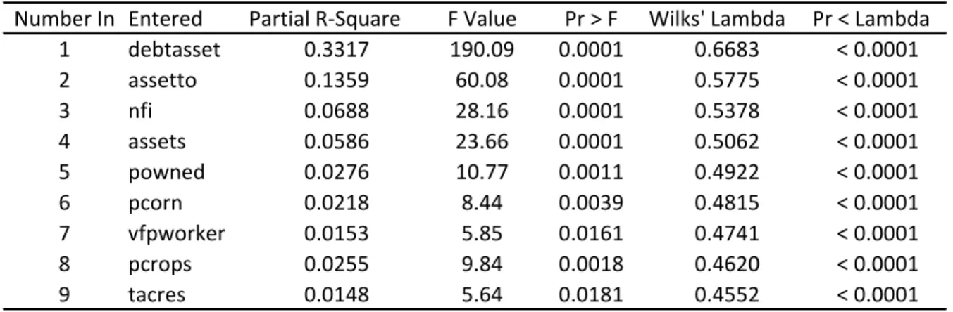
After means testing, discriminant analysis is used to determine whether age groups differ with regards to a variable mean. Basically, discriminant analysis asks whether two or more age groups are significantly different from each other with respect to particular variables. All variables will be tested in SAS using the STEPDISC procedure to determine which variables discriminate the most between age groups.
When using the STEPDISC procedure, it is assumed that the set of variables are to be multivariate normal with a common covariance matrix. Stepwise selection analysis is used to determine the relative contribution of each variable in terms of discriminating between groups. By using discriminant analysis, one can rank which variables discriminate the most between groups. Discriminant analysis will be conducted using all age groups, groups one and four, groups two and four, and groups three and four.
23
CHAPTER 4 - Data
This chapter will summarize the means and standard deviations of variables pertaining to farm size and tenure, specialization, efficiency, solvency and liquidity ratios used in this study. This chapter gives a general idea of what a typical farm operated by a sole proprietor in the Kansas Farm Management Association looks like.
Summary statistics for 964 KFMA farms classified as sole proprietors are presented in Table 4.1. To be included in this study, a farm had to be a member of the Kansas Farm
Management Association and had to have continuous, usable data for the 2002 to 2006 period. Using these five years of data, a cross-sectional data set was created by computing five-year averages for each farm. The four sections below discuss the summary statistics pertaining to the farm size and tenure variables, the specialization variables, the efficiency ratios, and the liquidity and solvency variables.
4.1. Farm Size and Tenure
Out of the 964 farms in this study, 194 were in group one, which contains farmers under 45 years of age. There were 298 farmers in group two with an operator age between 46 and 55. Group three contained 275 farmers with an operator age between of 56 and 65. Lastly, group four contained 197 farmers with an operator age over of 65. Percentage of farms from each area of the state (west, central, and east) for each age group was computed. Group one is broken down into west, central, and east with respective percents of 13.4%, 38.7%, and 47.9%. Group two contains farmers in the west, central, and east with respective percents of 14.1%, 41.9%, and 44.0%. Group three is broken down into west, central, and east with respective percents of
24
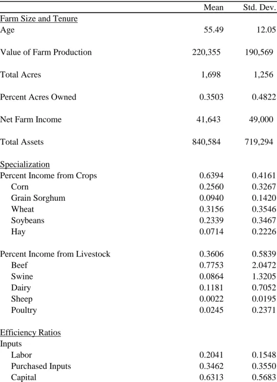
Table 4.1. Means and Standard Deviations of all Farmers.
Mean Std. Dev. Farm Size and Tenure
Age 55.49 12.05
Value of Farm Production 220,355 190,569
Total Acres 1,698 1,256
Percent Acres Owned 0.3503 0.4822
Net Farm Income 41,643 49,000
Total Assets 840,584 719,294
Specialization
Percent Income from Crops 0.6394 0.4161
Corn 0.2560 0.3267
Grain Sorghum 0.0940 0.1420
Wheat 0.3156 0.3546
Soybeans 0.2339 0.3467
Hay 0.0714 0.2226
Percent Income from Livestock 0.3606 0.5839
Beef 0.7753 2.0472 Swine 0.0864 1.3205 Dairy 0.1181 0.7052 Sheep 0.0022 0.0195 Poultry 0.0245 0.2371 Efficiency Ratios Inputs Labor 0.2041 0.1548 Purchased Inputs 0.3462 0.3550 Capital 0.6313 0.5683
25 Table 4.1. Continued. Mean Std. Dev. Efficiency Ratios Profit Margin 0.0876 0.2884 Return on Assets 0.0103 0.0614
Return on Assets with Capital Gains 0.0633 0.0632
Return on Equity -0.0305 0.2162
Return on Equity with Capital Gains 0.0736 0.2273
Asset Turnover 0.2621 0.2649
Value of Farm Production per Worker 178,859 250,683
Total Expense 0.8110 0.8224
Adjusted Total Expense 0.9805 0.8970
Economic Total Expense 1.1816 1.1147
Economic Total Expense with Capital Gains 0.9727 0.9082 Liquidity and Solvency
Inverted Current Ratio 0.4462 0.6962
26
12.4%, 34.9%, and 52.7%. Group four contains farmers in the west, central, and east with respective percents of 21.3%, 30.5%, and 48.2%.
Based on the USDA classification system, there were 227 farms in the first value of farm production group with value of farm production less than $100,000. There were 438 farms in the second value of farm production group with a value of farm production between $100,000 and $249,999. The third value of farm production group contained 247 farms with a value of farm production between $250,000 and $499,999. Lastly, the fourth value of farm production group had 52 farms with a value of farm production greater than $500,000.
The mean age of farmers in this data set was 55.49 years old. The average farm had a value of farm production of $220,355, classifying it as a farm in the second value of farm
production category. The average farm size of a sole proprietor in this study is 1,698 total acres, with the operator owning 35% of those acres. The average net farm income was $41,643. Total assets averaged $840,584 per farm.
4.2 Specialization
Specialization is used to determine what output mix farmers are producing. Percent income from crops was calculated by adding income from corn, grain sorghum, wheat, soybeans, and hay and dividing by the total income from crops and livestock. On average, 63.9% of
farmers income comes from producing crops. Percent income for individual crops was also computed by taking the individual crop income and dividing by total crop income. Wheat (32.6%), corn (25.6%), and soybeans (23.4%) contributed the most to crop income.
Percent income from livestock was calculated by adding beef, swine, dairy, sheep, and poultry income together and dividing by total income from crops and livestock. Individual livestock income was computed by taking individual livestock income and dividing it by total
27
livestock income. An overwhelming majority of livestock income came from beef (77.5%) with dairy (11.8%) and swine (8.6%) a distant second and third. It is important to note that beef includes backgrounding and cow-calf operations. A cow/feeder ratio was calculated by taking total cows divided by total feeders, where feeders include raised calves, for each age group. A higher ratio indicates that more income comes from cow/calf operations while a lower ratio indicates that more income comes from backgrounding. Group one had a cow/feeder ratio of 38.64%, group two 20.34%, group three 33.97%, and group four 40.51%. Based on this
information, group four produced the most income from cow/calf operations than the other three groups.
4.3 Efficiency Ratios
This section starts off by looking at the input mix of labor, purchased inputs, and capital inputs. The labor efficiency ratio was computed by adding paid and unpaid labor and dividing this total by value of farm production. The average labor efficiency ratio was 0.204. A lower number indicates that a farmer is efficiently using labor. Purchased inputs are calculated by taking purchased input expense and dividing by value of farm production. The average
purchased input expense ratio was 0.346. Lastly, capital inputs are computed by taking capital expense and dividing by value of farm production. The average capital input expense ratio was 0.631.
The operating profit margin ratio was calculated by adding net farm income plus interest expense minus unpaid labor dividing by value of farm production. Unpaid labor charge was computed using information on unpaid family labor, unpaid operator labor, and a management charge. The average unpaid labor was $37,355. This is decomposed into unpaid family labor of $1,587; unpaid operator labor of $24,396; and a management charge of $11,372. The average
28
profit margin was 0.088. Farms that have a negative profit margin ratio are not covering unpaid labor expense. Out of the 964 farms in this study, 35% had a negative profit margin.
The return on assets was computed by adding net farm income and interest expense minus unpaid labor and dividing by average total assets. The average return on assets was 0.010. Return on assets with capital gains was calculated by adding net farm income, interest expense, and capital gains, subtracting unpaid labor, and dividing by average total assets. The average return on assets with capital gains was 0.063. The return on equity was computed by subtracting unpaid labor from net farm income and dividing by net worth. The average return on equity was -0.031. The return on equity with capital gains was calculated by taking net farm income plus capital gains subtracting unpaid labor, and dividing by net worth. The average return on equity with capital gains was 0.074. Capital gains are solely based off of land appreciation. In the KFMA program, land is revalued every five years (e.g., 2000, 2005). Interpolation and the state average land values for 2000 and 2005 were used to create land values for each year. Land values were revised for each farm and capital gains were then computed by comparing land values from one year to the next.
The asset turnover ratio is computed by dividing value of farm production by total assets. The asset turnover ratio averaged 0.262. The next ratio computed was value of farm production per worker. It was calculated by dividing value of farm production by the number of workers. The average value of farm production per worker was $178,859. This ratio can be used to help measure labor efficiency. Operations that are relatively efficient in labor usage will have a relatively high value of farm production per worker.
The total expense ratio can be used as a financial efficiency measure. The total expense ratio equals total expense divided by value of farm production. The average total expense ratio
29
was 0.811. Adjusted total expense ratio equals total expense plus unpaid labor divided by value of farm production. The average adjusted total expense ratio was 0.981. A value below one indicates that a farm is covering operating expense, depreciation, and unpaid labor. Out of the 964 farms in this study, only 46% of the farms had an adjusted total expense ratio below one. This ratio indicates that a majority of farms are not covering unpaid labor.
The economic total expense ratio is another measure of financial efficiency that accounts for operating expense, depreciation, unpaid labor, and an owned asset charge. The economic total expense ratio equals total expense plus unpaid labor plus an opportunity charge on owned assets divided by value of farm production. The average economic total expense ratio was 1.180. An economic total expense ratio below one indicates that a farm is covering operating expense, depreciation, unpaid labor, and owned asset charges. A ratio below one signifies economic profit is being earned. Only 9.5% of the farms are earning an economic profit. The last efficiency ratio illustrated in Table 4.1 is the economic total expense ratio with capital gains. This ratio is computed by adding total expense, unpaid labor, and an interest charge on owned assets together and dividing by value of farm production plus capital gains. The average
economic total expense with capital gains ratio was 0.973. This indicates that capital gains play a significant role in lowering the economic total expense ratio. Out of the 964 farms in this study, 53% had an economic total expense ratio with capital gains below one.
4.4 Liquidity and Solvency
The current ratio had to be inverted because of farms with zero debt and therefore is listed as the inverted current ratio in all tables. For discussion purposes it was flipped back to the current ratio. The current ratio equals current assets divided by current liabilities. The average inverted current ratio was 0.446 which implies a current ratio of 2.24. A current ratio around two
30
is considered adequate and generally means short-term debts are covered by short-term assets. The debt to asset ratio measures the importance of borrowed funds in financing the farm‟s operations and is computed by dividing total debt by total assets. The average debt to asset ratio was 0.304.
31
CHAPTER 5 - Results
In this chapter t-test results will be summarized. Specifically, variables pertaining to farm size and tenure, specialization, efficiency, liquidity, and solvency ratios are compared across age groups using t-tests. Discriminant analysis is used to determine which variables are the most important in explaining differences among age groups.
5.1 T-Test Results
The t-tests were generated using the pooled method with equal variances in SAS to determine if the means of variables are significantly different among age groups. Unequal variances were also examined and were similar to the equal variance results. T-test results for one age group were compared to all other age groups.
An individual t-value will be positive if the first mean is larger than the second and negative if it is smaller. In order to find out whether the first mean is significantly different than the second mean, one needs to look and see if the probability is indicative of a p-value that is significantly different than zero at the 5% level. If the probability value is greater than 0.05, the variable means are not significantly different, but if the probability value is less than 0.05, the variable means are significantly different. Table 5.1 summarizes p-values pertaining to the age group comparisons.
In Table 5.2, if two groups have the same superscript letter there is no significant difference between the means, but if the two groups have different superscript letters it means there is significant difference between the means. Table 5.2 presents variable averages for each
32
Table 5.1. P-Values of Group Comparisons.
1 & 2 1 & 3 1 & 4 2 & 3 2 & 4 3 & 4 Farm Size and Tenure
Value of Farm Production 0.8976 0.6483 <.0001 0.6893 <.0001 <.0001
Total Acres 0.0097 0.0042 0.4574 0.5227 0.0010 0.0005
Percent Acres Owned 0.0210 <.0001 <.0001 <.0001 <.0001 <.0001 Net Farm Income 0.1719 0.1919 <.0001 0.9273 <.0001 <.0001
Total Assets 0.0011 <.0001 <.0001 0.0225 0.1619 0.3881
Specialization
Percent Income from Crops 0.9173 0.6623 0.7363 0.3718 0.7756 0.4311
Corn 0.0851 0.0292 0.0003 0.4156 0.0047 0.0763
Grain Sorghum 0.6529 0.7869 0.5478 0.9421 0.6897 0.3786
Wheat 0.1297 0.1774 0.0056 0.4405 0.0191 0.0351
Soybeans 0.6830 0.2811 0.6323 0.6549 0.3796 0.1513
Hay 0.6870 0.9991 0.4080 0.5376 0.4899 0.3480
Percent Income from Livestock 0.9173 0.6623 0.7363 0.7134 0.7756 0.4311
Beef 0.0654 0.0447 0.3317 0.5995 0.3454 0.3904
Swine 0.4220 0.7616 0.0562 0.0972 0.1925 0.0915
Dairy 0.0916 0.0060 0.2585 0.0972 0.1990 0.2585
Sheep 0.8983 0.0334 0.4666 0.0270 0.3738 0.1693
33
Table 5.1. Continued.
1 & 2 1 & 3 1 & 4 2 & 3 2 & 4 3 & 4 Efficiency Ratios Inputs Labor Efficiency 0.9723 0.1180 <.0001 0.058 <.0001 <.0001 Purchased Inputs 0.9847 0.4421 0.4509 0.3851 0.3935 0.8906 Capital 0.0002 <.0001 <.0001 <.0001 <.0001 <.0001 Profit Margin 0.0467 <.0001 <.0001 0.0017 <.0001 <.0001 Return on Assets 0.0035 <.0001 <.0001 0.073 <.0001 <.0001 Return on Assets + Capital Gains 0.0785 0.1199 0.0042 0.7126 0.0728 0.0274
Return on Equity 0.4019 0.1648 0.1633 0.2816 0.2290 0.8768
Return on Equity + Capital Gains 0.0251 0.0239 0.0084 0.7729 0.0813 0.2152 Asset Turnover <.0001 <.0001 <.0001 <.0001 <.0001 <.0001 Value of Farm Production per Worker 0.0804 0.0013 0.2420 0.1061 <.0001 <.0001
Total Expense 0.1580 0.1793 <.0001 0.9851 0.9523 0.9423
Adjusted Total Expense 0.4611 0.1102 <.0001 0.2260 <.0001 0.0012 Economic Total Expense 0.0069 <.0001 <.0001 0.0004 <.0001 <.0001 Economic Total Expense + Capital Gains 0.2932 0.2628 <.0001 0.9061 0.0001 0.0003 Liquidity and Solvency
Debt to Asset Ratio 0.1610 0.9306 0.0140 0.1328 0.0018 0.0135
34
Table 5.2. Variable Differences Among Age Groups.
Group 1 Group 2 Group 3 Group 4 Farm Size and Tenure
Value of Farm Production 245,303a 243,225a 236,407a 138,781b
Total Acres 1,530a 1,809b 1,879b 1,444a
Percent Acres Owned 0.2199a 0.2874b 0.3766c 0.5577d
Net Farm Income 50,613a 44,436a 44,042a 25,233b
Total Assets 640,205a 815,447b 965,655c 901,342bc
Specialization
Percent Income from Crops 0.6790a 0.6665a 0.5894a 0.6281a
Corn 0.3044a 0.2597ab 0.2321bc 0.2143c
Grain Sorghum 0.0892a 0.0961a 0.0895a 0.1075a
Wheat 0.2864a 0.3060a 0.3214a 0.3816b
Soybeans 0.2273a 0.2295a 0.2492a 0.2210a
Hay 0.0583a 0.0754a 0.0817a 0.0587a
Percent Income from Livestock 0.3209a 0.3334a 0.4105a 0.3718a
Beef 0.6233a 0.8349ab 0.7754b 0.8563ab
Swine 0.1060a 0.0206a 0.1551a 0.0190a
Dairy 0.2099a 0.1220ab 0.0657b 0.1228ab
Sheep 0.0037a 0.0026a 0.0011b 0.0015ab
35
Table 5.2. Continued.
Group 1 Group 2 Group 3 Group 4
Efficiency Ratios Inputs Labor Efficiency 0.1832a 0.1934a 0.2065a 0.2631b Purchased Inputs 0.3587a 0.3465a 0.3392a 0.3399a Capital 0.5186a 0.6050b 0.6460c 0.8618d Profit Margin 0.1164a 0.0901b 0.0958c 0.0110d Return on Assets 0.0446a 0.0269b 0.0235b 0.0017c
Return on Assets with Capital Gains 0.0896a 0.0790ac 0.0803ab 0.0709c
Return on Equity 0.0337a 0.0097a 0.0079a (0.0067)a
Return on Equity with Capital Gains 0.1151a 0.0893b 0.0899b 0.0635b
Asset Turnover 0.3831a 0.2982b 0.2448c 0.1539d
Value of Farm Production per Worker 207112a 190362ab 177776b 129327c
Total Expense 0.7936a 0.8172a 0.8136a 0.8181a
Adjusted Total Expense 0.9514a 0.9787a 0.9776a 1.0426b
Economic Total Expense 1.0605a 1.1451b 1.1918c 1.4648d
Economic Total Expense with Capital Gains 0.9491a 0.9747a 0.9672a 1.0106b
Liquidity and Solvency
Debt to Asset Ratio 0.4476a 0.345a 0.307a 0.0142b
Inverted Current Ratio 0.5173a 0.4589b 0.4909c 0.25714d
36
age group which can be compared to the all farm average in Table 4.1. Group one contains sole proprietors under or equal to age 45, group two contains farmers with ages between 46 and 55 years, group three contains farmers with ages between 56 and 65 years, and group four contains farmers over the age of 65.
5.1.1 Farm Size and Tenure
Variables are listed in the same order as they were in chapters three and four. This sub-section summarizes value of farm production, total acres, percent acres owned, net farm income, and total assets. The main comparisons of t-tests are between age groups one and four. The reason for focusing on these two groups is to demonstrate how different the two age group extremes are in efficiency and financial performance.
Based on the t-test results, groups one (less than or equal to 45 years of age), two (46 to 55 years of age), and three (56-65 years of age) all had similar values of farm production but group four (greater than 65 years of age) was significantly different. Group four had the lowest value of farm production with $138,781 and group one had the largest with $245,303. For total acres, age groups one and four were not significantly different, but group two and three were significantly different from these two groups. Age group four had the lowest total acre average with 1,444 acres, roughly 85 acres less than group one and 435 acres less than group three, which had the most acres.
All age groups had a significantly different percent acres owned. The fourth age group owns 56% of their total acres, which is more than double the 22% of total acres owned by the first age group. The fourth age group owns the highest percent of land among all age groups. Looking at net farm income, group four is half as profitable as group one. Group four has a net farm income of $25,233 while group one‟s net farm income is $50,613. The net farm income for
37
group four is also approximately $20,000 less than that for groups two and three. The final variable of this section is total assets. The fourth age group has the second largest asset base with $901,342, which is significantly different than the first age group, which has $640,205 of total assets.
After looking at the first five variables some interesting observations are worth noting. As one can see, the fourth age group of farmers has the least amount of land, owns the highest percent of that land, and has the second largest asset pool but is only half as profitable as the first age group. Profitability of the fourth age group is being severely limited by a combination of factors, some of which will be explained in the sub-sections below.
5.1.2 Specialization
This section summarizes percent income from crops and livestock. Income from crops includes income from corn, grain sorghum, wheat, soybeans, and hay. Income from livestock includes beef, swine, dairy, sheep, and poultry income. The purpose of this section is to determine whether one age group is more specialized in crops or livestock, and what crop or livestock mix they produce. Refer to Table 5.1 for exact comparison results.
The t-test results for percent income from crops show no significant difference between age groups. Group four produces 62.81% of their income from crops. Group one has the highest percentage of crop income with 67.90%. Group four had the most specialized farms, with 30% of their farmers growing only crops compared to group one with 19% growing only crops. A majority of the farmer‟s income comes from crops, and the following text will discuss which crops contribute to that income. T-test results show a significant difference in corn production between age groups one and four. The fourth age group had the lowest percentage of income
38
from corn (21.43%), while group one had the largest percentage with 30.44%. As farmers progressively got older they produced less corn.
With respect to percent income from wheat, group four was significantly different than the other groups. Group four had 38.16% of its crop income derived from wheat, while group one had 28.64%, which is 10% less wheat income than group four. Groups two and three were similar to group one. It is interesting to note the difference in crop mix between groups one and four. Group four produces more wheat than corn and group one is just the opposite. Grain sorghum, soybeans, and hay all had similar t-test results and there were no significant differences among age groups for these income sources.
Next, the percent income from livestock t-tests show no significant difference between age groups. The fourth age group had the second highest livestock income with 37.18%, topped only by the third age group with 41.05% of its income derived from livestock. The first age group had the lowest percent income from livestock with 32.09%. Group four had no farms solely specialized in livestock and group one had less than 1.0% that produced only livestock.
Beef constitutes the majority of income from livestock. For group four, 85.63% of their livestock income was derived from beef production. Age group one had the lowest percent of beef income with 62.33%. Although, beef income percents are different between groups one and four, t-test results show no significant difference. Swine plays a small role relative to beef in contributing to livestock income. The fourth age group gets 1.90% of its livestock income from swine, which is the lowest of all age groups. The first age group gets 10.60%, which is second highest in swine income. Despite there differences, t-test results show no significant difference among all age groups.
39
Group four derives 12.28% of its livestock income from dairy production, which is not significantly different from any other age group. Group one has the highest percent of dairy income with 20.99%, and is significantly different than group three with dairy income of 6.57%. Sheep play a relatively small role in percent income from livestock with all groups averaging below one percent. T-test results do not show a significant difference between any of the groups with respect to poultry income. There was no recorded income from poultry in the fourth age group. The first age group had the highest percent income from poultry with 6.39%.
5.1.3 Efficiency Ratios
The following section summarizes input mix, profit margin, asset turnover, rates of return, value of farm production per worker, and expense ratios, which were defined in previous chapters. This section also exposes more inefficiencies associated with the fourth age group.
The three inputs examined in this section are labor, purchased inputs, and capital. A large index for any input is an indication of inefficiency. The fourth age group has the highest labor efficiency index at 0.263 and is significantly different from all other age groups. Group one has the lowest labor efficiency index at 0.183, and is the most efficient group in terms of labor usage. This ratio demonstrates that the fourth age group is very inefficient in terms of labor usage. T-test results show no significant difference between purchased input indices among age groups. This illustrates that the age groups are using a comparable purchased input mix. The last input variable is capital. T-test results show that each age group is significantly different from the others. The capital input index is extremely high for the fourth age group with an index of 0.862. The first age group has the lowest capital input index with a value of 0.519. The differences between capital input indices illustrates that the fourth age group is using capital differently than group one.
40
T-test results indicate that the operating profit margin is significantly different among all age groups. The fourth age group has the lowest profit margin with a value of 0.011, while the first age group has the highest profit margin with a value of 0.116. This ratio indicates that over a five year period, the fourth age group has not been very profitable. As a matter of fact, 55% of the farms in group four have a negative profit margin while only 26% are negative in group one.
T-test results show significant differences among age groups for the return on asset ratio. Group four has the lowest return of 0.002, while group one has the highest return with a value of 0.045. This ratio indicates that group four is barely using their assets to generate earnings. Return on assets with capital gains indicates a significant difference between groups one and four. Group one had the highest value of 0.090 and group four had the second lowest value of 0.071. This shows by adding capital gains in the mix, the return on assets increases significantly. T-test results for return on equity was significantly higher for group one. Group one had the highest value of 0.034, while group four had a negative value of 0.007. This indicates that group four is not generating earnings on invested dollars. Return on equity with capital gains show no significant difference among age groups. By including capital gains with return on equity group four now generates earnings on invested dollars.
The asset turnover ratio showed that all age groups were significantly different from one another. The fourth age group had the lowest asset turnover ratio with a value of 0.154 and the first age group had the highest ratio with a value of 0.383. The asset turnover ratio results illustrate inefficiencies in asset utilization for farms in the fourth age group. Another important labor efficiency measure is value of farm production per worker. T-test results show that group four is significantly different from all other age groups with respect to this variable. While group
41
four has the smallest value of farm production per worker with a value of $129,327, group one had the highest value at $207,112. Results indicate that the fourth age group is inefficient in terms of labor usage.
The total expense ratio is not significantly different among age groups. Group four had a total expense ratio of 0.818 which is slightly higher than group one with a ratio value of 0.794. This ratio indicates all groups are covering operating expense and depreciation. T-test results for the adjusted total expense ratio show that group four is significantly different from all other groups. Group four had the highest ratio with a value of 1.043 while group one had the lowest value (0.951). This ratio shows that group four is not covering unpaid labor. As a matter of fact, only 32% of the farms in group four have an adjusted total expense ratio below one, compared to 57% in group one.
The economic total expense ratio produced interesting t-test results, with all age groups being significantly different from one another. The fourth age group had the highest economic total expense ratio with a value of 1.465 and group one had the lowest ratio value at 1.061. This ratio reveals the extreme differences between groups one and four. Although on average, no group is earning an economic profit, group four is having the hardest time covering labor and capital. Approximately, 27% of the farms in group one are earning an economic profit while there are zero farms in group four earning an economic profit. The last efficiency ratio is economic total expense ratio with capital gains. T-test results show that group four is
significantly different than the other three groups. Group four had an economic total expense ratio with capital gains value of 1.011, which is significantly higher than group one with a value of 0.949. The results are intriguing, because even by adding capital gains into the mix, group four still cannot cover labor and capital. As a matter of fact, only 42% of farms in group four