Zurich Open Repository and Archive University of Zurich Main Library Strickhofstrasse 39 CH-8057 Zurich www.zora.uzh.ch Year: 2017
Discrete-time option pricing with stochastic liquidity
Leippold, Markus ; Schärer, Steven
Abstract: Classical option pricing theories are usually built on the law of one price, neglecting the impact of market liquidity that may contribute to significant bid-ask spreads. Within the framework of conic finance, we develop a stochastic liquidity model, extending the discrete-time constant liquidity model of Madan (2010). With this extension, we can replicate the term and skew structures of bid-ask spreads typically observed in option markets. We show how to implement such a stochastic liquidity model within our framework using multidimensional binomial trees and we calibrate it to call and put options on the SP 500.
DOI: https://doi.org/10.1016/j.jbankfin.2016.11.014
Posted at the Zurich Open Repository and Archive, University of Zurich ZORA URL: https://doi.org/10.5167/uzh-128700
Journal Article Accepted Version
The following work is licensed under a Creative Commons: Attribution-NonCommercial-NoDerivatives 4.0 International (CC BY-NC-ND 4.0) License.
Originally published at:
Leippold, Markus; Schärer, Steven (2017). Discrete-time option pricing with stochastic liquidity. Journal of Banking and Finance, 75:1-16.
Discrete-time option pricing with stochastic liquidity
Markus Leippold∗ Steven Sch¨arer†
September 6, 2016
Abstract
Classical option pricing theories are usually built on the law of one price, neglecting the impact of market liquidity that may contribute to significant bid-ask spreads. Within the framework of conic finance, we develop a stochastic liquidity model, extending the discrete-time constant liquidity model of Madan (2010). With this extension, we can replicate the term and skew structures of bid-ask spreads typically observed in option markets. We show how to implement such a stochastic liquidity model within our framework using multidimensional binomial trees and we calibrate it to call and put options on the S&P 500.
JEL Classification: C51; D52; G12; G13
Keywords: Market Liquidity; Bid-Ask Spreads; Option Pricing; Stochastic Liquidity; Conic Finance
∗Department of Banking and Finance, University of Zurich, Switzerland. †Department of Banking and Finance, University of Zurich, Switzerland.
1
Introduction
Classical option pricing theories are usually based on the paradigm of complete and frictionless markets. However, even in financial markets that are considered to be highly competitive, we do observe drops in liquidity, which in times of financial turmoils may be significant and spark concerns among market participants. Liquidity has many different facets. In this paper, we measure liquidity as the spread between bid and ask prices. Illiquid assets are characterized by a high spread. When illiquidity draws a wedge between bid and ask prices, we can no longer rely on the law of one price. The first attempts to explain bid-ask spreads were made by introducing transaction costs such as
commission charges or inventory costs.1 However, these models often fail to explain the magnitude
of the spreads observed in the markets. Especially after the financial crisis of 2008, bid-ask spreads of many assets were persistently high and at a level that cannot be explained by transaction costs
alone.2 A different approach was taken by Madan and Cherny (2010) which is based on theory of
conic finance, originating from the work by Cherny and Madan (2009). The basic premise is that the market takes the role of a central counterparty that buys and sells assets from and to investors. The investor buys at the ask price and sells at the bid price. The difference of these prices gives rise to the bid-ask spread observed in financial markets. The central counterparty is viewed as passive in that it does not maximize some utility function, but rather carries out all trades that are acceptable to it.3
Madan and Cherny (2010) propose to model market illiquidity by a single market stress level parameter, according to which the market assigns bid and ask prices to assets based on the concept of acceptability indices. This static liquidity model was further extended and taken to the data in Corcuera, Guillaume, Madan, and Schoutens (2012) and Albrecher, Guillaume, and Schoutens (2013). These papers suggests at least two stylized facts for implied liquidity. First, market liquidity implied by real-world data exhibits both a skew and a term structure. This observation is in stark contrast to the assumption of a single liquidity parameter over all maturities and strikes. Second, 1See, e.g., Davis, Panas, and Zariphopoulou (1993), Shreve and Soner (1994), Soner, Shreve, and Cvitani´c (1995),
Cvitani´c and Karatzas (1996), Barles and Soner (1998).
2See, e.g., Pedersen (2009) for the average bid-ask spreads of large-cap U.S. stocks from June 2006 to June 2009. 3Acceptability itself is measured by acceptability indices, which are rooted in the theory of coherent risk measures
as developed in Artzner, Delbaen, Eber, and Heath (1999).
0.8 0.85 0.9 0.95 1 1.05 1.1 1.15 1.2 Moneyness 0.8 0.85 0.9 0.95 1 1.05 1.1 1.15 1.2 Normalized prices
Panel A: Bid-ask spread, put options
T = 3m T = 5m T = 11m
Jan-09 Jan-10 Jan-11 Jan-12 Jan-13
0 0.05 0.1 0.15 0.2 0.25 0.3 0.35
Bid-ask spread, normalized prices
Panel B: Put options
ITM OTM ATM
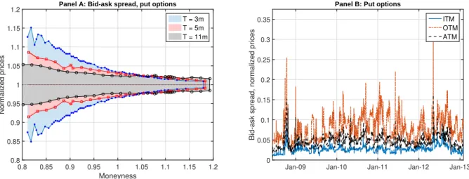
Figure 1. In Panel A, we plot the bid-ask spread for selected maturity slices of the European puts on the S&P 500 on July 20, 2012. We normalize the bid-ask spreads by the mid-prices. Moneyness is expressed as the ratio of strike over forward price. In Panel B, we plot the time-series of bid-ask spreads of in-the-money (ITM, 120% moneyness), out-of-the-money (OTM, 80% moneyness), and at-the-money (ATM, 100% moneyness) puts on the S&P500 with maturity of 5 months on July 20, 2012.
they show that when we calibrate a single market liquidity parameter for the S&P 500 option market, we obtain a time-series of the implied liquidity parameter with a mean-reverting stochastic behavior over time.
These stylized facts are illustrated in Figure 1. In Panel A, we plot the bid-ask spreads in terms of normalized prices of European puts written on the S&P 500 index. Clearly, bid-ask spreads differ across moneyness and time-to-maturity. In Panel B of Figure 1, we plot the historical bid-ask spreads for European puts with a maturity of five months. Clearly, these historical spreads change over time and exhibit some mean-reverting behavior. Hence, the empirical evidence presented in Corcuera, Guillaume, Madan, and Schoutens (2012) and Albrecher, Guillaume, and Schoutens (2013), together with the snapshot of historical bid-ask spreads in Figure 1, provides us with valuable guidance in designing a stochastic liquidity model that may account for the skew and term structure effects of implied liquidity.
We contribute to the steadily growing literature on liquidity modeling for option pricing in two ways. First, by making the setup of the discrete-time constant liquidity model of Madan (2010) more rigorous, we can simplify his results and extend the constant liquidity model to a stochastic liquidity framework. Our Theorem 1 allows us to represent bid and ask prices under stochastic liquidity given by backward recursions as time-consistent and dynamically translation invariant nonlinear
tions. This result opens the door to introduce stochastic liquidity in the conic finance framework. As an illustration, we apply a specific stochastic liquidity model using multidimensional binomial trees to the S&P 500 index option market. We show that this extension improves the fit of the term and skew structures in bid-ask spreads observed in markets. To the best of our knowledge, this is the first model to treat liquidity as a separate process that can be applied to the pricing of bid-ask spreads of derivatives. Compared to other approaches, our model is also suitable for deriving the bid and ask prices of path-dependent options such as Asian and Barrier options.
There have been various other endeavors on how to introduce dynamic bid-ask spreads in option pricing based on the model of Madan and Cherny (2010). An obvious way to do so is to model the bid and ask price as two separate stochastic processes, as suggested in Madan and Schoutens (2014). However, it can be considered a drawback that for payoffs which are not comonotone with a long or short stock position, this approach only gives lower and upper bounds for bid and ask prices. Another avenue is to follow the literature of dynamic risk measures. Mirroring the steps of the static one-step model, Bielecki, Cialenco, Iyigunler, and Rodriguez (2013) define dynamic acceptability indices with the help of dynamic coherent risk measures as discussed in, e.g., Riedel (2004) and Artzner, Delbaen, Eber, Heath, and Ku (2007). The disadvantage of using dynamic coherent risk measures is that they are not as tractable and intuitive compared to the static setup. It is furthermore not clear how a stochastic liquidity component could be incorporated. Biagini and Bion-Nadal (2014) tackle the issue in a similar way and arrive at a continuous-time version, while Bielecki, Cialenco, and Chen (2015) make use of Backward Stochastic Difference Equations (BS∆Es) and Rosazza Gianin and
Sgarra (2013) derive dynamic risk measures fromg-expectations.
Other than the approaches described above which are all based on or inspired by Conic Finance,
there is a large body of literature that explores liquidity and bid-ask spreads in option markets.4
One way to derive bid and ask prices of derivatives is by considering the replication costs induced
by an illiquid underlying. A popular model in this direction was conceived by C¸ etin, Jarrow, and
Protter (2004) who propose to model illiquidity by assuming that prices of underlyings are provided by a stochastic supply curve, that is not impacted by the actions of buyers and sellers. The resulting 4See, e.g., George and Longstaff (1993), Engle and Neri (2010), Chou, Chung, Hsiao, and Wang (2011), Chan and
Chung (2012), Bongaerts, De Jong, and Driessen (2011), Christoffersen, Goyenko, Jacobs, and Karoui (2015), and Feng, Hung, and Wang (2014), to name a few.
bid and ask prices are then dependent on the trade size which differs from our assumption of a trade-invariant bid-ask spread. They find that, in discrete time, hedging derivatives by trading the
illiquid underlying incurs liquidity costs. However, results in C¸ etin, Jarrow, Protter, and Warachka
(2006) indicate that this approach can only partially explain bid-ask spreads of derivatives observed in the market. In a separate study, Chou, Chung, Hsiao, and Wang (2011) also conclude that it is not sufficient to only consider the underlying’s liquidity, but also an option’s own liquidity must be taken into account. In contrast, our model does not specifically differentiate between underlying and option liquidity and indeed does not use replicating strategies to derive option prices. Hence, we assume that all information regarding liquidity is contained in the bid and ask prices of the option
market.5
The rest of the paper is structured as follows. In Section 2, we review the one-period framework of Madan and Cherny (2010). Section 3 introduces the multi-period model with stochastic liquidity. In Section 4, we bring our model to the data and show that the stochastic liquidity model helps to explain the skew and term structure typically observed in options’ bid ask spreads. Finally, Section 5 concludes. All proofs are delegated to the appendix.
2
One-step static liquidity model
We start with a brief description of the one-step liquidity model presented in Madan and Cherny (2010), since it builds the basis of our stochastic liquidity model presented in the subsequent section.
To this end, we fix a probability space (Ω,F,P) and denote by L∞ := L∞(Ω,F,P) the space of
all essentially bounded and R-valued random variables on (Ω,F,P).6 By P, we denote the
refer-ence probability measure that we assume to be a risk-neutral measure. In a complete market, this
probability measure is unique and the price of an asset is given by the P-expectation of its future
discounted cash flows, say Q ∈L∞. When market incompleteness drives a wedge between bid and
ask prices, we can interpret the bid (ask) price as being caused by an overweighting (underweighting) 5In our approach, we cannot differentiate between how much of the illiquidity reflected in the options’ bid-ask
spreads are due to the illiquidity of the underlying market and how much is due to the option market itself.
6This choice is for simplicity only and the results can be generalized toLpspaces with 1≤p <+∞. The
of losses and an underweighting (overweighting) of gains relative to the measure P. Hence, we can model this weighting scheme as a distortion to the reference probability measure. For this purpose, we define a distortion function as follows.
Definition 1 (Distortion function). A function ψ : [0,1] −→ [0,1] is a distortion function if and
only if it is monotone, ψ(0) = 0 and ψ(1) = 1.
The distorted probability measure ψ◦P is no longer a probability measure in general. It is,
however, still a finite monotone set function that is submodular, if the distortion function is concave. It is therefore possible to define a risk measure based on distorted probabilities using Choquet integrals.7
Definition 2 (Distortion risk measure). Let ψ be a concave distortion function and Q a future
discounted cash flow. The function ̺ψ :L∞−→R given by
̺ψ(Q) := Z 0 −∞ ψ(P(Q≤x))dx− Z ∞ 0 (1−ψ(P(Q≤x)))dx, ∀Q∈L∞, (1)
is called a distortion risk measure induced by ψ.
From the properties of the Choquet integral and because ψ◦P is submodular, the function ̺ψ
defined by equation (1) is monotone, positively homogeneous, translation invariant, and subadditive.
Hence, it is a coherent risk measure. By inverting the sign of̺ψ we obtain what is called a distorted
expectation, corresponding to the intuition of weighting losses and gains differently compared toP.
In particular, we call the function Eψ[·] :L∞−→Rgiven by
Eψ[Q] :=−̺ψ(Q), ∀Q∈L∞, (2)
the distorted expectation induced byψ.
Just as coherent risk measures,Eψ[·] is nonlinear, i.e., in generalEψ[Q1+Q2]6=Eψ[Q1]+Eψ[Q2] for
Q1, Q2 ∈L∞. Nevertheless, Eψ[·] shares many other properties with the usual expectation operator
such as monotonicity, positive homogeneity, and translation invariance. The concept of nonlinear 7See Choquet (1953). For more details on the properties of Choquet integrals, see the standard book of Denneberg
expectations, albeit in a multi-period setting, will be the cornerstone of our stochastic liquidity model.
In particular, from Definition 2 it follows that for Q∈L∞ andψ a concave distortion function,
Eψ[Q]≤E[Q]≤ −Eψ[−Q], (3)
whereE[·] denotes the expectation with respect to the reference pricing measureP. Hence, distorted
expectations provide an intuitive basis for the modeling of bid-ask spreads.
To measure the degree of distortion applied to the reference probability measure P, the central
counterparty is assumed to have not only one concave distortion function with which it evaluates
potential trades, but a whole family Ψ = (ψz)
z≥0. This family of concave distortion functions is
pointwise increasing in z in that ψz1(·) ≤ψz2(·) if and only if z
1 ≤z2. Additionally, ψ0 is assumed
to be the identity function. For a given distortion function ψγ ∈ Ψ under which cash flows are
evaluated, we can interpret γ as the market liquidity level. The more illiquid the market becomes
(i.e., the higher γ is), the more distorted the reference probability measure becomes. A liquidity
level of zero implies that no distortion at all is applied, which corresponds to perfect liquidity and
hence to the complete market case, in which the law of one price holds.8
A discounted cash flowQ∈L∞is deemed acceptable at γ if and only ifEψγ
[Q]≥0. The market
is assumed to competitively execute only acceptable trades. Therefore, the bid price bΨ,γ(Q) of a
discounted cash flowQ∈L∞ is the highest price the market is willing to pay for the net position to
be acceptable according to the market liquidity level, i.e.,
bΨ,γ(Q) := sup{b∈R|Eψγ[Q−b]≥0}=Eψγ[Q], (4)
where the last equality follows from the translation invariance of coherent risk measures. A similar
argument can be made for the ask price and leads to the following definition of bid and ask prices.9
Definition 3 (Single-period bid-ask prices). Let Ψ = (ψz)z≥0 be a pointwise increasing family of
concave distortion functions andγ >0 the market liquidity level. Then, the ask price of a discounted
8The liquidity measure in our model is not directly defined by observable variables in the market such as trading
volume or the bid-ask spreads. Instead, it is inferred from a comparison of market and model implied bid-ask spreads.
9This approach differs significantly from deriving bid and ask prices of derivatives based on a replicating trading
cash flow Q∈L∞ is given by aΨ,γ(Q) :=−Eψγ[−Q] = Z 0 −∞ (ψγ(P(Q > x))−1)dx+ Z ∞ 0 ψγ(P(Q > x))dx, (5)
and its bid price is
bΨ,γ(Q) :=Eψγ[Q] =− Z 0 −∞ ψγ(P(Q≤x))dx+ Z ∞ 0 (1−ψγ(P(Q≤x)))dx. (6)
Without any further assumptions, the bid price is always less than or equal to the ask price. Bid and ask price also envelop the undistorted price, i.e.,
bΨ,γ(Q)≤E[Q]≤aΨ,γ(Q) ∀Q∈L∞. (7)
Madan and Cherny (2010) derive these bid and ask prices from the theory of acceptability indices,
which are functions α : L∞ → [0,∞]. In particular, they call a net cash flow, or trade, Qe ∈ L∞
acceptable at a certain market liquidity levelγ if and only ifα(Qe)≥γ.10 Cherny and Madan (2009)
show that acceptability indices can be represented by a family of coherent risk measures (̺z)
z≥0
that are continuous from above and pointwise increasing in z. For a pointwise increasing set of
concave distortion functions Ψ = (ψz)
z≥0, such a family is given by the corresponding distortion risk
measures Φ = (̺ψz
)z≥0. To see that Φ is pointwise increasing inz, note that distortion risk measures
retain the ordering of the associated distortion function. Furthermore, all distortion risk measures
are continuous from above.11 Hence there exists an acceptability index which corresponds to Φ.
For our model, we assume the conditional value-at-risk (CVaR) as distortion measure.12
Accord-ing to, e.g., F¨ollmer and Schied (2011), the CVaR at levelα∈(0,1] can be expressed as a distortion
10Equivalently,aΨ,γ(Q) = sup
e
P∈DE
e
P[Q], whereD is the convex set of risk measures that are equivalent toP and
are determined byαandγ.
11See, e.g., F¨ollmer and Schied (2011).
12Other measures that have been applied in the literature are the Wang distortion function (Wang (2000)), the
MinMaxVar-distortion function introduced in Cherny and Madan (2009), or the EssSupExp-distortion function pro-posed by Bann¨or and Scherer (2014).
risk measure CVaRα(Q) =̺ψe α (Q) = Z 0 −∞ e ψα(P(Q≤x))dx− Z ∞ 0 (1−ψeα(P(Q≤x)))dx, ∀Q∈L∞, (8)
induced by the concave distortion function
e
ψα(u) := minnu α,1
o
, ∀u∈[0,1]. (9)
The distortion functions in our setup have to depend on a parameter taking values in [0,∞). However,
the quantile parameterαis defined on (0,1]. We therefore first use the change of variablesx7→1−x
to map (0,1] to [0,1) and then apply a sigmoid function, e.g.,
ϕ(x) := √ x
1 +x2, ∀x∈R, (10)
which bijectively maps values from [0,∞) to [0,1). With that we get, forz≥0 and α= 1−ϕ(z)∈
(0,1],
CVaRα(Q) =̺ψ
ϕ−1(1−α)
CVaR (Q) =̺ψCVaRz (Q) = CVaR1−ϕ(z)(Q), ∀Q∈L∞, (11)
for the modified concave distortion function
ψzCVaR(u) := min u 1−ϕ(z),1 , ∀u∈[0,1]. (12)
As required, the family ΓCVaR = (ψCVaRz )z≥0 is pointwise increasing in z and ψCVaR0 is the identity
function.
3
Discrete-time stochastic liquidity model
The model presented in the last section only considers a single time step. Hence, it is of limited practical value. In this section, we extend the model of Madan (2010) to treat market liquidity as a stochastic process instead of a constant to account for the stylized facts of bid and ask spreads. As in the static model, it is our goal to have bid and ask prices that are represented by nonlinear expectations. Due to the multi-period setup, we additionally require that they behave consistently
over time. These nonlinear expectations can also be used to define dynamic risk measures as we show in Remark A.1.
The proof of the main theorem, which we present in Appendix A, relies on the theory of BS∆Es of Cohen and Elliott (2010b), the discrete-time analogue of Backward Stochastic Differential Equations (BSDEs) as developed by El Karoui, Peng, and Quenez (1997). Similar to how Coquet, Hu, M´emin,
and Peng (2002) linked g-expectations to solutions of BSDEs, one can show that certain types of
nonlinear expectations are solutions to BS∆Es. As in the static setup, these will be used to define the bid and ask prices of discounted cash flows.
Before we present the main result, we introduce some additional notation. We denote by T > 0
maturity and assume we have time points 0 =t0 <· · · < tK = T for K >0. By Tij := Si≤l≤j{tl}
we denote the set of time points from ti to tj, where 0 ≤ i, j ≤ K. Let (Ω,F,(Ft)t∈TK
0 ,
P) be a
finite filtered probability space satisfying the usual conditions. The underlying price S = (St)t∈TK
0 is modeled as a positive but otherwise general finite state price process on the probability space (Ω,F,(Ft)t∈TK
0 ,
P). As in the static setting, P denotes the reference probability measure that is
assumed to be risk-neutral.
3.1 Time-consistent nonlinear expectations
In the spirit of Peng (2007), dynamic nonlinear expectations are defined as follows.
Definition 4 (Time-consistent nonlinear expectation). A family of functions E(· | Ft) :L1(FT)−→
L1(Ft) for t ∈ T0K is a time-consistent nonlinear expectation if it satisfies, for all s ∈ T0K and
Q, Q1, Q2 ∈L1(FT),
(i) monotonicity, i.e., if Q1≤Q2 P-a.s., then
E(Q1| Ft)≤ E(Q2| Ft) P-a.s
Additionally, for Q1≤Q2 P-a.s., equality holds if and only if P-a.s. Q1 =Q2. (ii) adaptability, i.e., E(Q| Ft) =Qif Q is Ft-measurable.
(iv) relevance, i.e., 1AE(Q| Ft) =E(1AQ| Ft),P-a.s. ∀A∈ Ft.
The monotonicity property states that of two different payoffs, the one that isP-a.s. smaller also
has a smaller expectation under E(· | Ft) for allt∈ T0K. Adaptability is assumed due to our
multi-period setup. Dynamic consistency is what is known as the tower property for usual conditional expectations. For nonlinear expectations, we have to explicitly make this assumption to ensure that
different time steps are linked consistently. Finally, “relevance” means that at time t, the investor
knows whether the underlying’s path is in A ∈ Ft. If this is the case, the nonlinear expectation of
1AQ is the same as the one ofQ. Otherwise, it is zero.
Definition 5(Dynamic translation invariance). A time-consistent nonlinear expectation(E(· | Ft))t∈TK
0
is dynamically translation invariant if and only if for all t∈ TK
0 ,
E(Q+q| Ft) =E(Q| Ft) +q, ∀Q∈L1(FT), q∈L1(Ft). (13)
Dynamic translation invariance is not generally required of nonlinear expectations. Nevertheless, we want to ensure that, e.g., a portfolio consisting of one derivative and some cash has the same bid price as adding the cash to the bid price of the derivative on its own.
3.2 Distorted conditional expectation
Instead of considering only a constant market liquidity level γ as in Madan (2010), we introduce a
stochastic process to model market liquidity through time and states.
Definition 6 (Market liquidity process). The time- and state-dependent process Γ = (γt)t∈TK
0 , for γt∈L1(Ft) andγt≥0 P-a.s. for all t∈ T0K is called market liquidity process.
Before, we used the liquidity level γ ≥ 0 to determine the degree of distortion applied to P by
choosing ψγ from a family of pointwise increasing concave distortion functions Ψ. We will continue
in this spirit, but since the liquidity level at any time is now a random variable, we introduce a state-dependent distortion function.
called a concave state-dependent distortion function if and only if for allω ∈Ω, ψ(ω,·) is a concave distortion function.
Slightly abusing notation, we will denote by Ψ := (ψz)
z≥0 the usual family of concave distortion
functions that are pointwise increasing inz and define, for a random variable γ,
ψγ(ω, u) :=ψγ(ω)(u) ∀ω∈Ω, u∈[0,1]. (14)
This gives a concave state-dependent distortion function as defined above. As such, we will continue working with the same family of concave distortion functions as in the previous section. The notion of distorted expectations is also extended to state-dependent distortion functions. Furthermore, they are now conditional on the filtration.
Definition 8 (Distorted conditional expectation). Let ψ be a concave state-dependent distortion
function. The family of functions with elements Eψt[·] : L1(FT) −→ L1(Ft) for t ∈ T0K, defined
∀Q∈L1(F T) and∀ω ∈Ω as Eψt[Q](ω) :=− Z 0 −∞ ψ(ω,Pt(Q≤x)(ω))dx+ Z ∞ 0 1−ψ(ω,Pt(Q≤x)(ω))dx (15)
is called distorted conditional expectation.
For brevity, we denote the conditional probability by13
Pt(A) :=P(A| Ft) =E[1A| Ft], ∀A∈ FT.
Since Pt(·)(ω) is a probability measure for any state ω ∈ Ω and t ∈ TK
0 , E
ψ
t[·](ω) is a distorted
expectation as in the static framework. As in the static case it holds that
Eψt[Q]≤E[Q| Ft]≤ −Eψt[−Q], P-a.s., (16)
for all Q∈L1(F
T),t∈ T0K, and all concave state-dependent distortion functionsψ.
13Note that we assume enough regularity on (Ω,F,(F
t)t∈TK
0 ,
P) that a regular conditional distribution can be constructed.
3.3 Time-consistent bid and ask prices
To define the bid and ask prices in our multiperiod setting, we borrow from the one-step static
liquidity model of Madan and Cherny (2010). We start at the final maturity T and recursively
apply the conditional distorted expectation. The stochastic liquidity component thereby determines the re-weighting of the reference probability measure depending on the current state and time step.
Working backwards, we arrive at timet0 and obtain today’s bid and ask prices.
Definition 9 (Multi-period bid-ask prices). For Ψ := (ψz)z≥0 a family of concave distortion
func-tions that are pointwise increasing in z, market liquidity process Γ = (γt)t∈TK
0 and tk∈ T
K
0 , the bid price of a future discounted cash flowQ∈L1(F
T) at time tk is defined as bΨt,Γ k (Q) :=E ψγtk tk [E ψγtk+1 tk+1 [· · ·E ψγtK−1 tK−1 [Q]]]. (17)
Its ask price at time tk is given by
aΨtk,Γ(Q) :=−Eψtγtk k [E ψγtk+1 tk+1 [· · ·E ψγtK−1 tK−1 [−Q]]]. (18)
The distorted conditional expectation does not satisfy the tower property. Hence, it is not a time-consistent nonlinear expectation. Therefore, bΨt,Γ(Q) 6=Eψtγ[Q] in general. However, it is still adapted, monotone and dynamically translation invariant, as also Lemma A.2 shows. By accounting for the dynamic translation invariance of the driver in the BS∆E, we are able to simplify the result in Madan (2010) and prove that the bid and ask prices from Definition 9 are time-consistent and
dynamically translation invariant nonlinear expectations.14 At the same time, we correct an error in
the proof of Madan (2010), see Remark A.2.
Theorem 1. Let Ψ := (ψz)
z≥0 a family of concave distortion functions that are pointwise increasing in z and Γ = (γt)t∈TK
0 a market liquidity process. Then, the bid and ask prices (b
Ψ,Γ
t )t∈TK
0 and
(aΨt,Γ)t∈TK
0 are time-consistent and dynamically translation invariant nonlinear expectations. 14 Time-consistency of bid and ask prices prevents round-trip arbitrage opportunities. In particular, buying Q at
timet0 has to cost the same as buying a newly introduced asset that pays the ask price ofQat timet1. This payoff
3.3.1 Constant liquidity model
As a first application of Theorem 1, we can consider a constant liquidity model. In particular, by
fixing γ >0 to a constant, we obtain the model suggested by Madan (2010) albeit with simplified
expressions for the bid and ask price. Assuming a recombining binomial tree model for the stock price process (Stk)
K
k=0 with a constant time step size h:= KT, and k= 1, ..., K,
Stk :=S0u
Pk
i=1ξidk−Pki=1ξi, (19)
whereS0>0,u≥1,d= 1/uand (ξi)Ki=1 are iid random variables with values in{0,1}, for which we
set the up and down probabilitiespu:=P(ξi= 1), pd:=P(ξi = 0). We also have a family of concave
distortion functions Ψ that are pointwise increasing. For option payoffs that are path-dependent, it is necessary to go through the tree backward recursively to calculate the bid and ask prices at time zero. For other payoffs such as European vanilla contracts, it is possible to derive closed-form expressions. Given Theorem 1, we obtain the following analytical formulas for the bid and ask prices of European claims.
Corollary 1. Let the future discounted cash flow be given by a function H such that Q=H(T, ST).
Further assume that H is non-negative and monotonically increasing with ST (e.g., a European call
option). Then, aΨ0,γ(Q) = K X i=0 K i ψγ(pu)i(1−ψγ(pu))K−iH(T, S0uidK−i) (20) and bΨ0,γ(Q) = K X i=0 K i (1−ψγ(pd))iψγ(pd)K−iH(T, S0uidK−i). (21)
Similarly, for a non-negative but monotonically decreasing payoff (e.g., a European put option), we have aΨ0,γ(Q) = K X i=0 K i ψγ(pd)i(1−ψγ(pd))K−iH(T, S0uK−idi) (22) and bΨ0,γ(Q) = K X i=0 K i (1−ψγ(pu))iψγ(pu)K−iH(T, S0uK−idi). (23)
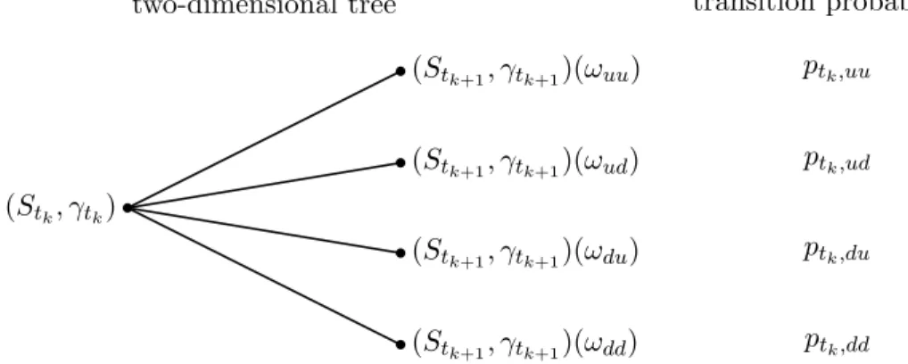
two-dimensional tree transition probabilities ptk,uu ptk,ud ptk,du ptk,dd (Stk, γtk) (Stk+1, γtk+1)(ωuu) (Stk+1, γtk+1)(ωud) (Stk+1, γtk+1)(ωdu) (Stk+1, γtk+1)(ωdd)
Figure 2. A single node of the two-dimensional binomial tree for (S, γ) with the corresponding transition probabilities.
3.3.2 Stochastic liquidity model
To generalize the previous model to a stochastic liquidity model, we proceed as follows. We describe
the dynamics of S and γ by a two-dimensional recombining binomial tree (St, γt, pt, qt)t∈TK
0 as
il-lustrated in Figure 2. For any node (Stk, γtk), there are four connected nodes (Stk+1, γtk+1)(ωuu), (Stk+1, γtk+1)(ωud), (Stk+1, γtk+1)(ωdu) and (Stk+1, γtk+1)(ωdd) with corresponding transition proba-bilities ptk,uu, ptk,ud, ptk,du and ptk,dd. State ωud stands for an up-move of the underlying S and a
down-move of the liquidity processγ. The other states and transition probabilities are denoted using
the same notation.
We are now interested in calculating the bid and ask price of a future discounted cash flow
Q ∈ L1(FT) occurring at time T. For simplicity, we restrict ourselves to non-negative Q. Sinceγ
is non-constant, we cannot derive closed-form formulas for the bid and ask price as in the constant liquidity case. We therefore have to calculate them backward recursively according to Definition 9. To that end, we define bΨtK,Γ(Q) =aΨtK,Γ(Q) =Q withtK =T. Assuming we have already calculated
bΨt,Γ
k+1(Q) and a
Ψ,Γ
tk+1(Q), we can calculate bid and ask prices for every node of the previous time-step
as follows. First, starting from a node (Stk, γtk), we sort the four possible states ωuu,ωud,ωdu, and
ωdd such that bΨt,Γ k+1(Q)(ω b 1)≥bΨ ,Γ tk+1(Q)(ω b 2)≥bΨ ,Γ tk+1(Q)(ω b 3)≥bΨ ,Γ tk+1(Q)(ω b 4) (24) and aΨtk,+1Γ(Q)(ωa1)≥aΨtk,+1Γ(Q)(ωa2)≥aΨtk+1,Γ(Q)(ω3a)≥atΨk,+1Γ(Q)(ω4a), (25)
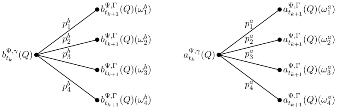
bΨt,γ k (Q) pb 1 bΨtk,+1Γ(Q)(ωb 1) pb2 bΨtk,+1Γ(Q)(ωb 2) pb 3 bΨt,Γ k+1(Q)(ω b 3) pb 4 bΨt,Γ k+1(Q)(ω b 4) aΨt,γ k (Q) pa 1 aΨtk,+1Γ(Q)(ωa 1) pa2 aΨtk,+1Γ(Q)(ωa 2) pa 3 aΨt,Γ k+1(Q)(ω a 3) pa 4 aΨt,Γ k+1(Q)(ω a 4)
Figure 3. The same node but now the states and transition probabilities are sorted such that the bid resp.
ask prices are highest forωb
1 resp. ω
a
1 and lowest forω
b
4resp. ω
a 4.
for statesωib, ωia∈ {ωuu, ωud, ωdu, ωdd},i= 1, ...,4. In Figure 3, we plot the node for the bid and ask
price. To simplify notation, we denote the transition probabilities corresponding to the states with
the same sub- and superscripts. Then, sinceQis non-negative, the bid price is given by
bΨt,Γ k (Q) =E ψγtk tk [b Ψ,Γ tk+1(Q)] = b Ψ,Γ tk+1(Q)(ω b 1)(1−ψγtk(p2b +pb3+pb4)) +bΨtk,+1Γ(Q)(ωb2)(ψγtk(pb 2+pb3+pb4)−ψγtk(pb3+pb4)) +bΨtk,+1Γ(Q)(ωb3)(ψγtk(pb 3+pb4)−ψγtk(pb4)) +bΨt,Γ k+1(Q)(ω b 4)ψγtk(pb4) (26)
and the ask price is
aΨtk,Γ(Q) =−Eψtγtk k [−a Ψ,Γ tk+1(Q)] = a Ψ,Γ tk+1(Q)(ω a 1)ψγtk(pa1) +aΨt,Γ k+1(Q)(ω a 2)(ψγtk(pa1+pa2)−ψγtk(pa1)) +aΨt,Γ k+1(Q)(ω a 3)(ψγtk(pa1+pa2+pa3)−ψγtk(pa1 +pa2)) +aΨtk,+1Γ(Q)(ω4a)(1−ψγtk(pa 1+pa2+pa3)). (27)
Continuing the backward recursion through the tree and applying the re-weighting of the reference
probability measure according to the distortion function, we can calculate the bid and ask price of any non-negative future discounted cash flow at any point in time.
4
Application
To illustrate our methodology, we consider European options written on the S&P 500 index and we calibrate both a static and a stochastic liquidity model, as defined in Sections 3.3.1 and 3.3.2, to
the bid-ask spreads of European index options.15 All data comes from the OptionMetrics database
accessed via the Wharton Research Data Services. For the calibration exercise, we choose as arbitrary
date July 20, 2012. The S&P 500 had a closing price of S0 = 1362.66 and the European options
market was neither particularly stressed nor overly relaxed. At this day, the option data consists of 2560 calls and puts with maturities ranging from 7 days to 2.4 years and a strike interval of 100 to 3000. We removed 295 options from the dataset for whose mid price no Black-Scholes implied volatility could be calculated. For our discussion, we restrict our analysis to calls and puts within
the [80%,120%] forward moneyness interval. Furthermore, we focus only on three maturities slices,
namely on maturities of three, five, and eleven months. This leaves us with a total of 230 calls and puts.
4.1 Model specification
For our application, we assume that the log returns of the index are conditionally normal
dis-tributed.16 For the liquidity process, we either assume it be constant for the static liquidity model
or consider a mean-reverting square-root process following the findings of Albrecher, Guillaume, and Schoutens (2013) regarding the behavior of the static liquidity model parameter over time. In
particular, for the stochastic liquidity model of Section 3.3.2, the asset priceS = (St)t∈TK
0 and the
liquidity process Γ = (γt)t∈TK
0 are binomial tree approximations of the continuous-time processes
dSt = St(r−q)dt+StσWtS S0 >0, (28)
dγt = κ(θ−γt)dt+ν√γtdWtγ, γ0>0, (29)
15Using the same techniques, it is also possible to model bid and ask prices of path-dependent payoffs.
16This choice is merely for illustration purposes. We are well aware of the fact that there are more suitable choices
for the underlying process. However, while, e.g., a stochastic volatility model such as the Heston model may be better suited, the imprecision in the volatility surface fit interferes with the assessment of the performance of the liquidity model.
where WS and Wγ are correlated Brownian motions with dhWS, Wγit =ρdt,ρ ∈[−1,1]. Byr we
denote the one-period risk-free rate, q the dividend yield, and σ the asset volatility. To improve
speed and memory usage, we prune the trees similar as in Baule and Wilkens (2004). For more
details on the construction of the binomial trees, we refer to Appendix B. The asset price S in the
static liquidity model is the same binomial tree approximation of (28) and the construction of the
binomial tree follows similarly, except that γ is a constant now.
Following Madan, Pistorius, and Stadje (2015), we modify the usual concave distortion function
ψγ to take into account the step size hof the tree via
ψγ,h(u) :=u+√h(ψγ(u)−u), ∀u∈[0,1], (30)
which is still concave. Using this adjustment allows for an adequate comparison of parameter esti-mates for the market liquidity process for different step sizes and in particular the one-step static
liquidity model. As distortion measure, we use CVaR.17
4.2 Calibration
In the following, we only refer to the calibration of the stochastic liquidity model. The calibration of the static model follows the same methodology and only differs in the constructed binomial tree (one-dimensional instead of two-dimensional) and number of liquidity parameters (one instead of five).18
Considering the available data in the different slices, it is evident that they are not equally distributed over either moneyness nor maturity. For example, the three month slices have over twice as many data points as the either of the other two and the eleven months moneyness interval [110%, 112%] contains over 20% of all data points despite being only 5% of the whole interval. To ensure a better fit over the whole moneyness range and not just areas with clustered strikes, we therefore
calculate regularly interpolated bid and ask prices, Pbid
i and Piask for i∈ {1, ..., M}, for each slice.
17We also conducted our analysis by using different measures. The differences were insignificant.
18We remark that for our calibration exercise we follow the standard practice of calibrating, e.g., a stochastic
volatility model, i.e., we treat the current level of liquidity as an additional parameter. A time-series estimation of implied liquidity would require setting up, e.g., a suitable filter method, which is beyond the scope of this paper.
These interpolated prices, instead of the real ones, will be used in our optimization algorithm below. The reported model fit in Table 1 and all figures will be based on real data.
We calibrate our model for each selected maturity slice of calls and puts separately. First, we
calculate for each option i∈ {1, ..., M}the Black-Scholes implied volatility σi such that
1 2(P
ask
i +Pibid) =BS(S0, Ki, Ti, ri, qi, σi),
whereKi andTi are the strike and time-to-maturity of optioni, respectively,ri is the zero rate with
maturity closest to Ti and qi is the implied dividend rate from the put-call parity.19 Furthermore,
we denote the market bid and ask prices by Piask and Pibid. For every option, the implied volatility
parameter is then used to construct the binomial tree for the underlying together with the correlated
tree for the liquidity process.20 The risk-free rate, dividend yield and the liquidity parameters,
including the correlation parameter ̺, are the same over all options of the selected maturity slice
while the implied volatility is allowed to be different to best replicate the observed market data.
Having fixed the distortion functions Ψ = (ψz)
z≥0 and a market liquidity process Γ in (29), which
depends on the set of parameters Θ ={γ0, κ, θ, ν, ρ}, we can calibrate the model by minimizing the
root-mean-square error (RMSE) of the normalized bid-ask spreads:21
RMSE(Θ|Ψ,Γ) := v u u t 1 M M X i=1 ∆Pmodel i −∆Pimarket 1 2(Pibid+Piask) !2 , (31)
where ∆Pimarket and ∆Pimodel are the market and model bid-ask spreads and M is the number
of options. The model bid and ask prices are calculated by starting at the terminal cash flows and applying equations (26) respectively (27) backward recursively throughout the two-dimensional 19Inferring the dividend yield from the put-call parity partially circumvents problems caused by different quotation
times from the option and underlying markets. The implied dividend yield for all options lies in the interval [1.90%, 2.21%]. The dividend yield reported in the OptionMetrics database is 2.50%.
20We remark that this procedure is only an approximation as the undistorted price is usually not exactly half-way
between the bid and ask price in our model. The approximation becomes cruder when getting closer to maturity and further away from at the money. Nevertheless, compared to the alternative of having to calibrateM additional parameters, the error from this approach seems acceptable.
21We also tested minimizing the spreads in implied volatility, but found that the improved fit in the implied volatility
space led to a, comparatively, bigger error in the normalized price space. Minimizing the model errors of the bid and ask prices respectively implied volatilities instead of the spreads did not lead to vastly different results.
0.8 0.85 0.9 0.95 1 1.05 1.1 1.15 1.2 Moneyness 0 0.05 0.1 0.15 0.2 0.25 0.3 0.35 0.4 Liquidity parameter, γ
Panel A: Call options
T = 3m T = 5m T = 11m 0.8 0.85 0.9 0.95 1 1.05 1.1 1.15 1.2 Moneyness 0.02 0.04 0.06 0.08 0.1 0.12 0.14 Liquidity parameter, γ
Panel B: Put options
T = 3m T = 5m T = 11m
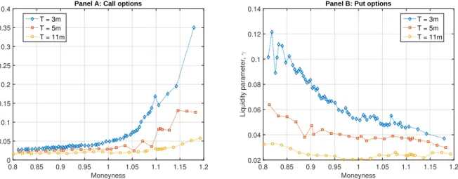
Figure 4. Market implied liquidity skew for selected maturity slices of the European options market on the S&P 500 on July 20, 2012. In total, we have 115 calls and the same number of puts. For every option, we
calculate the static market liquidity parameter γ, which minimizes the bid-ask spread. We use the CVaR
distortion function and assume a lognormal model for the underlying index.
binomial tree to get
∆Pimodel:=aΨ0,Γ(Qi)−bΨ0,Γ(Qi), (32)
whereQi is the cash flow associated to theith option.22
To avoid the problem of local minima, we use a surrogate model based on radial basis functions.23
Surrogate models are widely used in engineering because they require significantly less function evaluations than, e.g., genetic algorithms or particle swarm methods.
We first determined reasonable parameter ranges and optimized over these.24 To help the
numer-ical algorithm find better solutions, we then tightened the parameter ranges by determining where the best and worst model fits occurred. We tried to keep the parameter ranges as wide as possible to prevent influencing the final results too much.
4.3 Results and discussion
To motivate the use of a stochastic liquidity component, we first consider a static liquidity model as in Section 3.3.1 for which we regard every option in isolation. For the CVaR distortion function,
we calculate for every option i ∈ {1, ..., M} the unique parameter γi such that the model bid-ask
spreads calculated using Corollary 1 coincide with the market bid-ask spreads. In Figure 4, we plot
the calibrated liquidity parameter γ for various maturity slices and levels of moneyness. Clearly,
this market-implied liquidity parameter is far from being constant. It increases with decreasing maturity and when the option becomes out-of-the-money. Furthermore, the skew effect weakens
with increasing maturity.25
Going one step forward, we calibrate our stochastic liquidity model given in equation (29). As in the static model, we calibrate each maturity slice separately. Table 1 reports the parameter estimates and the RMSEs for the calibration of three maturity slices. As in the static case, the current implied
liquidity levelγ0 decreases with increasing maturity. Furthermore, liquidity shocks tend to be highly
transitory, which is reflected by the high values for the estimates of the parameterκ. These values
fit well our observation of the bid-ask spreads over time in Panel B of Figure 1. The persistence
of liquidity shocks, however, tends to increase with increasing maturity. The volatility estimate ν
decreases with increasing maturity. We find that for call options the long-term mean θ is almost
at the same level for all three maturities. For puts, we find a similar pattern, except for the eleven
months maturity slice. Finally, the estimates for the correlation parameter ρ indicate a consistent
and rather strongly negative correlation between changes in price and liquidity. Such high values make intuitively sense, as in times of highly negative returns such as, e.g., during the global financial
crisis in 2008-2009 and the European crisis in 2012, bid-ask spreads also widened significantly.26
For comparison, we have also calibrated the static liquidity model for which all options on the 22For the static liquidity model the relevant formulas are collected in Corollary 1.
23See Gutmann (2001) and in particular the toolbox MATSuMoTo developed by Mueller (2014). 24γ ∈[0.5γ∗
,2γ∗],
κ∈(0,100], θ ∈(0,0.05], ν∈ (0,2],̺∈(−1,1). γ∗ denotes the optimal liquidity parameter in the static model, see the next section for more details.
25These properties of the implied liquidity parameterγ is in line with what has been observed in the static one-step
models used in Albrecher, Guillaume, and Schoutens (2013) and Corcuera, Guillaume, Madan, and Schoutens (2012).
26The high correlation value corroborates the findings in Albrecher, Guillaume, and Schoutens (2013) of a high static
Stochastic liquidity model Static model
Type Mat γ0 κ θ ν ρ RMSE γ∗ RMSE
call 3m 0.151 22.823 0.008 0.980 -0.951 9.4% 0.170 20.1% call 5m 0.068 11.278 0.012 0.719 -0.974 3.4% 0.074 10.1% call 11m 0.031 18.903 0.011 0.553 -0.983 1.4% 0.029 3.8% put 3m 0.087 8.567 0.009 0.910 -0.975 1.2% 0.082 3.4% put 5m 0.036 4.220 0.010 0.726 -0.952 0.7% 0.045 1.6% put 11m 0.021 4.123 0.016 0.509 -0.977 0.6% 0.026 1.0%
Table 1. The table reports the calibrated parameters for European call and put options with different
maturities (Mat) on the S&P 500 on July 20, 2012, for the stochastic liquidity model and the static model. The underlying distortion function is chosen to be CVaR. The parameters of the liquidity process are estimated by minimizing the RMSE of the normalized bid-ask spreads.
selected maturity slices are fitted simultaneously. The optimal static liquidity parameter γ∗ turns
out to be of similar magnitude than the estimatedγ0 in the stochastic liquidity model. However, the
model fit is considerably worse, with an RMSE often more than twice as large as the RMSE from the stochastic model. This leads us to the conclusion that the stochastic liquidity model can lead to significant improvements statistically, while also representing more closely stylized facts about
market liquidity.27
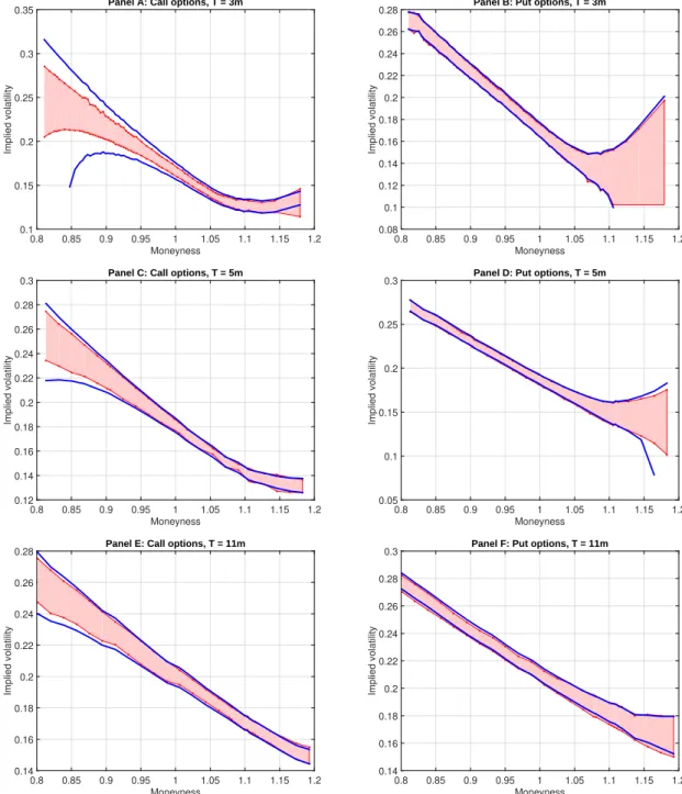
To further illustrate our model’s capability of fitting ask spreads, we plot in Figure 5 the bid-ask prices of calls and puts in terms of implied volatilities. We first observe that the general behavior of the data is well replicated by the model for all slices and both option types. The model performs worse for shorter maturities, where spreads are also generally larger than for longer maturities. However, especially for short-term OTM put options, the bid-ask spread is fitted remarkably well. In contrast, as can be observed in Figure 6, the static model struggles to replicate the bid-ask spread at short maturities. Especially the errors for ITM options tend to be substantial.
27As an additional exercise, we have re-calibrated our model on October 10, 2008, in the wake of the financial crisis.
Most parameters were all of the same order of magnitude. The calibration yielded parametersθandνthat were higher than on July 20, 2012. Furthermore, the current level of liquidity γ0 was also larger. We attribute this observation
to the increased uncertainty in the market at the time and the much wider bid-ask spreads, especially for puts. The observations that κis much higher for calls than puts and that ν decreases with maturity also held on October 10, 2008. Comparing with the static liquidity model, the RMSE was again improved by a factor of about two to three.
Moneyness 0.8 0.85 0.9 0.95 1 1.05 1.1 1.15 1.2 Implied volatility 0.1 0.15 0.2 0.25 0.3
0.35 Panel A: Call options, T = 3m
Moneyness 0.8 0.85 0.9 0.95 1 1.05 1.1 1.15 1.2 Implied volatility 0.08 0.1 0.12 0.14 0.16 0.18 0.2 0.22 0.24 0.26
0.28 Panel B: Put options, T = 3m
Moneyness 0.8 0.85 0.9 0.95 1 1.05 1.1 1.15 1.2 Implied volatility 0.12 0.14 0.16 0.18 0.2 0.22 0.24 0.26 0.28
0.3 Panel C: Call options, T = 5m
Moneyness 0.8 0.85 0.9 0.95 1 1.05 1.1 1.15 1.2 Implied volatility 0.05 0.1 0.15 0.2 0.25
0.3 Panel D: Put options, T = 5m
Moneyness 0.8 0.85 0.9 0.95 1 1.05 1.1 1.15 1.2 Implied volatility 0.14 0.16 0.18 0.2 0.22 0.24 0.26
0.28 Panel E: Call options, T = 11m
Moneyness 0.8 0.85 0.9 0.95 1 1.05 1.1 1.15 1.2 Implied volatility 0.14 0.16 0.18 0.2 0.22 0.24 0.26 0.28
0.3 Panel F: Put options, T = 11m
Figure 5. Calibration fit in the implied volatility space for European calls and puts on the S&P 500 on July 20, 2012. We plot the bid-ask spreads for maturities of 3, 5, and 11 months. We use the CVaR distortion function. The parameters of the liquidity process are estimated by minimizing the RMSE of the normalized bid-ask spreads. The shaded area corresponds to the market bid-ask spreads. The solid line corresponds to the model-implied spread.
Moneyness 0.8 0.85 0.9 0.95 1 1.05 1.1 1.15 1.2 Implied volatility 0.05 0.1 0.15 0.2 0.25 0.3 0.35 0.4
0.45 Panel A: Call options (static), T = 3m
Moneyness 0.8 0.85 0.9 0.95 1 1.05 1.1 1.15 1.2 Implied volatility 0.08 0.1 0.12 0.14 0.16 0.18 0.2 0.22 0.24 0.26
0.28 Panel B: Put options (static), T = 3m
Figure 6. Calibration fit for the European call and put three months maturity slice on the S&P 500 on July 20, 2012. Panel A plots the bid-ask spread for calls, Panel B plots the spread in the implied volatility space for puts. The distortion function is chosen to be CVaR. The shaded area corresponds to the market bid-ask spreads. The solid line corresponds to the model-implied spread.
4.4 Parameter sensitivities
To gain more insights into the different roles of the parameters determining the liquidity process, we perform a sensitivity analysis for the put option with 5 months to maturity. Using the parameter values from Table 1, we assume different values for one parameter while keeping all others fixed. Figures 7 and 8 illustrate the sensitivities in the implied volatility and the normalized price space. Market implied bid-ask volatilities and prices correspond to the dashed lines marked with asterisks and are interpolated from S&P500 data on July 20, 2012.
Panels A and B of Figure 7 plot the impact of changes in the current liquidity level γ0. As
expected, high illiquidity, i.e., a large value for γ0, is reflected by a wider bid-ask spread. For low
values of γ0, the spread collapses. In the implied volatility space, we note that the level of liquidity
seems to impact options across all levels of moneyness in a similar way, i.e., by a parallel move of
the implied volatility curve. Panels C and D plot the impact of changes in the parameterκ. Finally,
in Panels E and F we plot the impact of changes in the parameter θ. Both parameters relate to the
drift of the liquidity process. As forγ0 in Panel A, we observe that changes in these parameters lead
to a parallel move in the implied volatility surface. For more persistent liquidity shocks, i.e., a high
value forκ, the bid-ask spread widens and it further does so when the long term mean for illiquidity
0.8 0.85 0.9 0.95 1 1.05 1.1 1.15 1.2 Moneyness 0.1 0.15 0.2 0.25 0.3 0.35 Implied volatility
Panel A: Sensitivity for γ
0 0.8 0.85 0.9 0.95 1 1.05 1.1 1.15 1.2 Moneyness 0.7 0.8 0.9 1 1.1 1.2 1.3 1.4 Normalized prices
Panel B: Sensitivity for γ
0 0.8 0.85 0.9 0.95 1 1.05 1.1 1.15 1.2 Moneyness 0.12 0.14 0.16 0.18 0.2 0.22 0.24 0.26 0.28 0.3 Implied volatility
Panel C: Sensitivity for κ
0.8 0.85 0.9 0.95 1 1.05 1.1 1.15 1.2 Moneyness 0.8 0.85 0.9 0.95 1 1.05 1.1 1.15 1.2 Normalized prices
Panel D: Sensitivity for κ
0.8 0.85 0.9 0.95 1 1.05 1.1 1.15 1.2 Moneyness 0.12 0.14 0.16 0.18 0.2 0.22 0.24 0.26 0.28 0.3 Implied volatility
Panel E: Sensitivity for θ
0.8 0.85 0.9 0.95 1 1.05 1.1 1.15 1.2 Moneyness 0.75 0.8 0.85 0.9 0.95 1 1.05 1.1 1.15 1.2 1.25 Normalized prices
Panel F: Sensitivity for θ
Figure 7. Sensitivity analysis for different parameter values. The figure plots the changes in the implied volatility and normalized price curve of the put option with 5 month maturity when we change the underlying liquidity parameters. Market implied bid-ask volatilities and prices correspond to the dashed lines marked with asterisks and are interpolated from S&P500 data on July 20, 2012. Panels A and B plot the impact of
changes inγ0. Solid (dashed) lines and squares (circles) correspond to γ0 = 0.01 (γ0= 0.2). Panels C and D
plot the impact of changes in the parameterκ. Solid (dashed) lines marked with squares (circles) correspond
to κ= 1 (κ= 30). Panels E and F plot the impact of changes in the parameterθ. Solid (dashed) lines and
squares (circles) correspond toθ = 0.001 (θ= 0.1). For all graphs, the remaining parameters were set equal
0.8 0.85 0.9 0.95 1 1.05 1.1 1.15 1.2 Moneyness 0.1 0.12 0.14 0.16 0.18 0.2 0.22 0.24 0.26 0.28 0.3 Implied volatility
Panel A: Sensitivity for ν
0.8 0.85 0.9 0.95 1 1.05 1.1 1.15 1.2 Moneyness 0.85 0.9 0.95 1 1.05 1.1 1.15 1.2 Normalized prices
Panel B: Sensitivity for ν
0.8 0.85 0.9 0.95 1 1.05 1.1 1.15 1.2 Moneyness 0.12 0.14 0.16 0.18 0.2 0.22 0.24 0.26 0.28 0.3 Implied volatility
Panel C: Sensitivity for ρ
0.8 0.85 0.9 0.95 1 1.05 1.1 1.15 1.2 Moneyness 0.8 0.85 0.9 0.95 1 1.05 1.1 1.15 Normalized prices
Panel D: Sensitivity for ρ
Figure 8. Sensitivity analysis for different parameter values. The figure plots the changes in the implied volatility and normalized price curve of the put option with 5 month maturity when we change the underlying liquidity parameters. Market implied bid-ask volatilities and prices correspond to the dashed lines marked with asterisks and are interpolated from S&P500 data on July 20, 2012. Panels A and B plot the impact
of changes in the parameter ν. Solid (dashed) lines marked with squares (circles) correspond to ν = 0.25
(ν = 0.15). Panels C and D plot the impact of changes in the parameter ρ. Solid (dashed) lines and squares
(circles) correspond to ρ=−0.9 (ρ = 0.9). For all graphs, the remaining parameters were set equal to the
values given in Table 1.
In Figure 8 we plot the sensitivities with respect to the volatility of the liquidity processνand the
correlation between price changes and liquidity ρ. Here, we observe that the effect differs from the
previous analysis in Figure 8 in that there is a less pronounced parallel impact on implied volatility.
Instead, a change in the liquidity volatility parameterν leads to a sharp increase in the convexity of
the implied volatility of ask prices. Such an effect, but to a lesser extent, can also be observed for
5
Conclusion
Particularly after the financial crisis, the issue of market liquidity has been center stage for researchers and practitioners alike. However, the literature on liquidity in option markets and the discussion on how to incorporate liquidity into the pricing problem has been sparse. We add to this literature by providing a theoretical framework that allows us to incorporate a stochastic liquidity process into the option pricing problem. By specifying a simple version of our model and taking it to the data, we find that the additional flexibility of having a stochastic liquidity component helps to replicate the bid and ask spreads typically observed in option markets.
In our empirical exercise, we focus on a very simple and illustrative example. Hence, it comes at no surprise that our calibration analysis indicates some challenging avenues for future research. For example, the lack of fit at short-maturities corroborates the need for adding a jump component to the liquidity process. Furthermore, it may be advantageous to model the underlying process using a stochastic volatility model which, of course, leads to challenging numerical problems. A natural candidate for such an extension could be the recombining stochastic volatility tree of Akyıldırım, Dolinsky, and Soner (2014) as starting point. Inspired by the findings of Chou, Chung, Hsiao, and Wang (2011) it could be beneficial to consider a two-factor liquidity model, where one factor corresponds to the illiquidity of the underlying and the other to the illiquidity in the option market. Finally, one could go beyond a simple calibration exercise and try to perform a time-consistent estimation of the liquidity process using time series data. We leave these extensions to our analysis for future research.
References
Akyıldırım, Erdin¸c, Yan Dolinsky, and H Mete Soner, 2014, Approximating stochastic volatility by
recombinant trees, The Annals of Applied Probability 24, 2176–2205.
Albrecher, Hansjoerg, Florence Guillaume, and Wim Schoutens, 2013, Implied liquidity: Model
sensitivity,Journal of Empirical Finance 23, 48–67.
Artzner, Philippe, Freddy Delbaen, Jean-Marc Eber, and David Heath, 1999, Coherent measures of
risk,Mathematical Finance 9, 203–228.
, and Hyejin Ku, 2007, Coherent multiperiod risk adjusted values and Bellman’s principle,
Annals of Operations Research 152, 5–22.
Bann¨or, Karl F, and Matthias Scherer, 2014, On the calibration of distortion risk measures to bid-ask
prices,Quantitative Finance 14, 1217–1228.
Barles, Guy, and Halil Mete Soner, 1998, Option pricing with transaction costs and a nonlinear
Black-Scholes equation, Finance and Stochastics 2, 369–397.
Baule, Rainer, and Marco Wilkens, 2004, Lean trees - A general approach for improving performance
of lattice models for option pricing, Review of Derivatives Research 7, 53–72.
Biagini, Sara, and Jocelyne Bion-Nadal, 2014, Dynamic quasi concave performance measures,Journal
of Mathematical Economics 55, 143–153.
Bielecki, Tomasz R, Igor Cialenco, and Tao Chen, 2015, Dynamic conic finance via backward
stochas-tic difference equations, SIAM Journal on Financial Mathematics 6, 1068–1122.
Bielecki, Tomasz R, Igor Cialenco, Ismail Iyigunler, and Rodrigo Rodriguez, 2013, Dynamic conic finance: Pricing and hedging in market models with transaction costs via dynamic coherent
ac-ceptability indices, International Journal of Theoretical and Applied Finance 16, 1350002.
Bongaerts, Dion, Frank De Jong, and Joost Driessen, 2011, Derivative pricing with liquidity risk:
C¸ etin, Umut, Robert Jarrow, Philip Protter, and Mitch Warachka, 2006, Pricing options in an
ex-tended Black Scholes economy with illiquidity: Theory and empirical evidence,Review of Financial
Studies 19, 493–529.
C¸ etin, Umut, Robert A Jarrow, and Philip Protter, 2004, Liquidity risk and arbitrage pricing theory,
Finance and Stochastics 8, 311–341.
Chan, Kalok, and Y. Peter Chung, 2012, Asymmetric price distribution and bid–ask quotes in the
stock options market, Asia-Pacific Journal of Financial Studies 41, 87–102.
Cherny, Alexander, and Dilip Madan, 2009, New measures for performance evaluation, Review of
Financial Studies 22, 2571–2606.
Choquet, Gustave, 1953, Theory of capacities, inAnnales de l’Institut Fourier vol. 5 pp. 131–295.
Chou, Robin K, San-Lin Chung, Yu-Jen Hsiao, and Yaw-Huei Wang, 2011, The impact of liquidity
on option prices, Journal of Futures Markets 31, 1116–1141.
Christoffersen, Peter, Ruslan Goyenko, Kris Jacobs, and Mehdi Karoui, 2015, Illiquidity premia in
the equity options market,Working Paper.
Cohen, Samuel N, and Robert J Elliott, 2010a, Comparisons for backward stochastic differential
equations on Markov chains and related no-arbitrage conditions,The Annals of Applied Probability
20, 267–311.
, 2010b, A general theory of finite state backward stochastic difference equations, Stochastic
Processes and their Applications 120, 442–466.
, 2011, Backward stochastic difference equations and nearly time-consistent nonlinear
expec-tations, SIAM Journal on Control and Optimization 49, 125–139.
Coquet, Fran¸cois, Ying Hu, Jean M´emin, and Shige Peng, 2002, Filtration-consistent nonlinear
Corcuera, Jose Manuel, Florence Guillaume, Dilip B Madan, and Wim Schoutens, 2012, Implied
liquidity: towards stochastic liquidity modelling and liquidity trading, International Journal of
Portfolio Analysis and Management 1, 80–91.
Cvitani´c, Jakˇsa, and Ioannis Karatzas, 1996, Hedging and portfolio optimization under transaction
costs: A martingale approach, Mathematical Finance 6, 133–165.
Davis, Mark HA, Vassilios G Panas, and Thaleia Zariphopoulou, 1993, European option pricing with
transaction costs, SIAM Journal on Control and Optimization 31, 470–493.
Denneberg, Dieter, 1994, Non-Additive Measure and Integral (Springer).
El Karoui, Nicole, Shige Peng, and Marie Claire Quenez, 1997, Backward stochastic differential
equations in finance, Mathematical Finance 7, 1–71.
Engle, Robert, and Breno Neri, 2010, The impact of hedging costs on the bid and ask spread in the
options market, Unpublished Working Paper, New York University.
Ethier, Stewart N, and Thomas G Kurtz, 2009,Markov Processes: Characterization and Convergence
(John Wiley & Sons).
Feng, Shih-Ping, Mao-Wei Hung, and Yaw-Huei Wang, 2014, Option pricing with stochastic liquidity
risk: Theory and evidence,Journal of Financial Markets 18, 77–95.
F¨ollmer, Hans, and Alexander Schied, 2011, Stochastic Finance: An Introduction in Discrete Time
(Walter de Gruyter).
George, Thomas J, and Francis A Longstaff, 1993, Bid-ask spreads and trading activity in the S&P
100 index options market, Journal of Financial and Quantitative Analysis 28, 381–397.
Gutmann, Hans-Martin, 2001, A radial basis function method for global optimization, Journal of
Global Optimization 19, 201–227.
Madan, Dilip B, 2010, Conserving capital by adjusting deltas for gamma in the presence of skewness,
, and Alexander Cherny, 2010, Markets as a counterparty: An introduction to conic finance,
International Journal of Theoretical and Applied Finance 13, 1149–1177.
Madan, Dilip B, Martijn Pistorius, and Mitja Stadje, 2015, On dynamic spectral risk measures and
a limit theorem, arXiv preprint arXiv:1301.3531.
Madan, Dilip B, and Wim Schoutens, 2014, Two processes for two prices, International Journal of
Theoretical and Applied Finance 17, 1450005.
Mueller, Juliane, 2014, MATSuMoTo: The MATLAB surrogate model toolbox for computationally
expensive black-box global optimization problems, arXiv preprint arXiv:1404.4261.
Pedersen, Lasse Heje, 2009, When everyone runs for the exit,International Journal of Central
Bank-ing.
Peng, Shige, 2007, G-expectation, G-Brownian motion and related stochastic calculus of Itˆo type, in
Stochastic Analysis and Applicationsvol. 2 . pp. 541–567 (Springer).
Riedel, Frank, 2004, Dynamic coherent risk measures, Stochastic Processes and their Applications
112, 185–200.
Rosazza Gianin, Emanuela, and Carlo Sgarra, 2013, Acceptability indexes via g-expectations: an
application to liquidity risk, Mathematics and Financial Economics 7, 457–475.
Shreve, Steven E, and H Mete Soner, 1994, Optimal investment and consumption with transaction
costs, The Annals of Applied Probability 4, 609–692.
Soner, Halil M, Steven E Shreve, and J Cvitani´c, 1995, There is no nontrivial hedging portfolio for
option pricing with transaction costs,The Annals of Applied Probability 5, 327–355.
Wang, Shaun S, 2000, A class of distortion operators for pricing financial and insurance risks,Journal
A
Proof of Theorem 1
In the next two sections, we will summarize the theory of nonlinear expectations as solutions to BS∆Es on general discrete-time processes as developed by Cohen and Elliott (2010b). This frame-work is then used to show that the bid and ask prices from Definition 9 are in fact time-consistent and dynamically translation invariant nonlinear expectations as claimed in Theorem 1.
The log-price process of the underlying is denoted by X = (Xt)t∈TK
0 which, likeS, is a general
discrete-time, finite state process. Cohen and Elliott (2010b) developed the theory for terminal con-ditions with multi-dimensional payoffs, but we will only present their results for the one-dimensional
case. Additionally, while we assume without loss of generality that there are N ∈N states at each
time pointt∈ TK
0 , it is worth noting that the theory can be extended to infinite states (see Cohen
and Elliott (2011)), even though this is less relevant for our application which uses binomial trees.
A.1 BS∆E setup
Without loss of generality, we will set X0 = 0 and assume that each Xtk, tk ∈ T
K
1 , takes values in
the standard basis ofRN, i.e.,
Xtk ∈ {e1,· · ·, eN}, ej := (0,· · · ,0,1,0,· · ·,0)
⊤∈RN,
where ej is one at the j-th component and (·)⊤ denotes the transposition operator. We call the
processM := (Mtk)
K
k=0 defined by
Mtk :=Xtk−E[Xtk| Ftk−1]∈R
N, k= 1, ..., K (33)
and M0:= 0 the martingale difference process.
Definition A.1 (BS∆E). Let (Y, Z) := (Yt, Zt)t∈TK
0 be
R×RN-valued adapted processes, F : Ω×
TK
0 ×R×RN −→Ran adapted function and Qan R-valued,FT-measurable random variable.