The
Elasticity
of
Taxable
Income
in
New
Zealand
Iris Claus, John Creedy and Josh
Teng
Working
Paper
Series
July 2010
Research
Paper
Number
1104
ISSN:
0819
‐
2642
ISBN:
978
‐
0
‐
7340
‐
4458
‐
7
Department of Economics
The University of Melbourne
The Elasticity of Taxable Income in New Zealand
∗
Iris Claus
†, John Creedy
‡and Josh Teng
§Abstract
This paper reports estimates of the elasticity of taxable income with respect to the net-of-tax rate for New Zealand taxpayers. The elasticity of taxable income was estimated to be substantially higher for the highest income groups. Generally it was higher for men than for women. Changes in the timing of income flows for the higher income recipients were found to be an important response to the announcement of a new higher-rate bracket. The marginal welfare costs of personal income taxation were consistent across years, being relatively small for all but the higher tax brackets. For the top marginal rate bracket of 39 per cent, the welfare cost of raising an extra dollar of tax revenue was estimated to be well in excess of a dollar. Furthermore, for the top bracket the marginal tax rate was often found to exceed the revenue-maximising tax rate.
JEL Classification: H24; H31
Keywords: Income taxation; Taxable income; Elasticity of taxable income; Ex-cess burden of taxation.
∗We are grateful to the Royal Society of New Zealand for funding support from the Cross
Depart-mental Research Pool from Government, and Matt Benge and Sandra Watson for valuable comments. We have also benefited from suggestions by participants at seminars at the New Zealand Inland Rev-enue and the New Zealand Association of Economists 2010 conference. The views expressed in this paper are our own and not necessarily those of the Inland Revenue.
†Policy Advice Division, New Zealand Inland Revenue and Centre for Applied Macroeconomic
Analysis, Australian National University
‡Department of Economics, University of Melbourne, Victoria 3010, Australia. E-mail:
jcreedy@unimelb.edu.au.
This paper reports new estimates for New Zealand of the elasticity of taxable in-come with respect to the marginal net-of-tax rate. This elasticity aims to capture, in a ‘reduced-form’ relationship, all potential responses to income taxation in a single elasticity measure, without the need to specify the structural nature of the various adjustment processes involved.1 These adjustments include, as well as labour supply
changes, income shifting between sources which are taxed at different rates, and tax evasion through non-declaration of income. The elasticity of taxable income has the added attraction that, under certain assumptions, it can easily be used to obtain a measure of the excess burden of income taxation.
The estimates are obtained using a special dataset, constructed using a random sample of administrative data collected by the New Zealand Inland Revenue. The details of the sample method and the variables obtained are provided in Appendix A. The basic concept is introduced in Section 2, which describes the estimation meth-ods used in later sections. Section 3 briefly discusses the marginal rate structure of New Zealand’s income tax system. This has remained relatively stable since the middle 1990s. A major change was made in 2001, when a new top marginal rate was intro-duced. From 2001 until 2008, no threshold or marginal rate changes took place. Hence, a policy change and the existence offiscal drag provide two alternative approaches to estimating the elasticity. Section 4 concentrates on estimates obtained by considering the introduction of the 39 per cent rate, and Section 5 examines the implications of fiscal drag, whereby some individuals experience a change in their marginal rate on moving into a higher tax bracket. Brief comparisons with other estimates are made in Section 6. The welfare effects, arising from the tax distortion leading to the taxable income responses, are considered in Section 7. Further background details regarding welfare effects for all tax brackets are given in Appendix B, and summary informa-tion regarding the distribuinforma-tion of taxable income is contained in Appendix C. Brief 1The seminal contribution is by Feldstein (1995). The attraction of the measure is indicated by the
fact that a recent survey of estimates, by Saez, Slemrod and Giertz (2009), includes 111 references. For an introduction to the basic analytics, see Creedy (2009).
conclusions are in Section 8.
2
The Elasticity and Estimation
The central concept examined here is the elasticity, , of declared income, , with respect to the marginal net-of-tax rate, 1−. This is defined as:
= 1−
(1−) (1)
This elasticity captures all possible responses to tax rate changes in a single measure, without attempting to model each form of response. A popular constant-elasticity reduced-form specification is the following:2
=0(1−)
(2) where 0 denotes the individual’s income in the absence of taxation (that is, when
= 0). The remainder of this section describes the alternative estimation methods used in this paper.
Let and0 denote declared income of person at time and the income which
would be declared in the absence of taxation. Furthermore, is the marginal tax rate
facing individualat time , equal to () where ()is the tax function. Using the constant elasticity form given above:
=0(1−)
(3) where by assumption the elasticity is the same for all individuals in the relevant population group considered.3
One approach is to consider actual policy changes in the tax structure for which only a relatively small group of individuals are affected, using information about the 2It can be shown that this follows from an assumption that utility takes the quasi-linear form
= −³1+11 ´ ³ 0 ´1+1
, where is disposable income. Thus income effects of tax changes are assumed to be zero.
3Given information about
and for a group of individuals, a simple regression oflog on
log (1−)and a constant, thereby omitting the unobservable0, cannot be expected to provide a
there is a change in only the top marginal income tax rate, which has no effect on those subject to lower rates. Let denote the share of income of the affected group at time
, and their average marginal tax rate at is . Let = 0 and = 1 denote
pre-and post-change periods. If the share of income in the relevant group would have remained constant in the absence of the policy change, an estimate of , denoted ˆ, can be obtained using:
ˆ
= log1−log0
log (1−1)−log (1−0)
(4) This method requires only summary data relating to the (cross-sectional) taxable in-come distribution in two periods.
An alternative approach to a policy change involves using a difference-in-difference framework with panel data. However, the ‘control’ and ‘treatment’ groups cannot be identified in the usual way since in the present context they are defined by in-come. Suppose that the treatment group, , comprises the top 1 percentile of the income distribution and the control group,, is made up of individuals in the next2
percentile. Being in the treatment group clearly depends on the behaviour and char-acteristics of taxpayers. Again, suppose tax policy changes from period0 to period1, and let()denote the respective sample average. The appropriate difference between groups in the differences between average log-taxable income from one period to the next, denoted ∆log, is given by:
∆log ={( log1|)−( log0|)}−{( log1|)−( log0|)} (5)
The difference between groups in the differences between the logarithm of average net-of-tax rates from one period to the next, denoted∆log (1−), is given by:
∆log (1−) = {( log (1−1)|)−( log (1−0)|)}
−{( log (1−1)|)−( log (1−0)|)} (6)
The estimate of the elasticity of taxable income, ˆ, can be obtained using:
ˆ
= ∆log
Again, this approach involves an assumption that without the policy change the in-comes of the two groups would have grown at the same rate.4 In addition, the elasticity
of taxable income is assumed to be the same for both groups.
The difference-in-difference approach can also be applied in situations where there is no explicit policy change affecting the marginal tax rate faced by some individuals. In particular,fiscal drag gives rise to a general increase in average tax rates but it can also shift some individuals into the next bracket and thus subject them to a higher marginal rate. Such individuals are regarded as being in the ‘treatment’ group. Those in the lower section of an income range do not face a higher marginal rate, as they do not cross a threshold, and are regarded as being in the ‘control’ group. The expression forˆcan thus be used in this context. This method can be applied for each tax bracket, thereby allowing for variations in with income (between brackets).5
3
New Zealand’s Income Tax System
As mentioned earlier, the relative stability of the personal income tax structure, in terms of marginal rates and thresholds, provides helpful conditions for attempting to estimate the elasticity of taxable income. This section briefly discusses New Zealand’s income tax system.
New Zealand’s income tax system was transformed with economic reforms that be-gan in 1984. These reforms were designed to improve efficiency while raising revenue by broadening the tax base and lowering marginal income tax rates; see, for example, Evans et al. (1996). The tax base was broadened by introducing a comprehensive goods and services tax (GST) and a fringe benefit tax, and by eliminating many tax concessions, exemptions and investment and export incentives. The top personal mar-4If systematic income changes occur for non-tax reasons, for example if there is some ‘regression
towards the mean’ over time, the estimator may be biased. A method of allowing for such changes is examined by Creedy (2009).
5In addition to income tax thresholds, the real value of other tax parameters (such as allowance
and deduction limits) can fall during inflation, as examined by Onrubia and Sanz (2009). However, this is unlikely to be an issue in New Zealand given the limited allowances and deductions over the period of estimation.
0% 5% 10% 15% 20% 25% 30% 35% $0 $9,500 $30,8 75 $34 ,200 $38,0 00
1994 to 1996 1997 (composite year) 1998 1999 (composite year) 15% 33% 24% 26.25% 25% 28% 21.75%
Figure 1: Effective Tax Rates 1994 to 1999
ginal income tax rate was cut from 66 per cent to 33 per cent and the number of tax brackets was reduced from eleven to three. The company tax rate was lowered from 48 per cent to 33 per cent. Aggregate tax revenue actually increased despite the reductions in the tax rates.
The tax scales for 1994 to 1999 and 2000 to 2008 are plotted in Figures 1 and 2. The ‘composite’ years, 1997 and 1999, are years when a tax rate or income threshold change came into effect during the income tax year, which starts on 1 April and ends on 31 March.
New Zealand’s broad based, low rate personal income tax system introduced dur-ing the economic reforms remained virtually unchanged until 2001, although durdur-ing 1994 to 2001 the middle income tax bracket was subject to some threshold and rate adjustments. However, in 2001 a new top personal marginal tax rate of 39 per cent for income above $60,000 was introduced, with the company and trust rates remaining at 33 per cent.6 This policy change provides a useful natural experiment for studying the responsiveness of taxpayers to changes in marginal tax rates.
0% 5% 10% 15% 20% 25% 30% 35% 40% 45% $0 $9,500 $38,0 00 $60, 000 2000 2001 to 2008 15% 39% 33% 21%
Figure 2: Effective Tax Rates 2000 to 2008
Furthermore, over the period 2001 to 2008 no threshold or rate changes were made to the other tax brackets.7 As a result of income growth, with thresholds beingfixed in
nominal terms, a large number of taxpayers experienced an increase in their marginal rate because they moved into a higher tax bracket. Thesefiscal drag effects enable the difference-in-differences estimator discussed in the previous section to be used.
4
Empirical Results: Introduction of 39 Per cent
Rate
This section presents estimates of taxpayers’ responses to changes in marginal tax rates, following the introduction of the 39 per cent top personal marginal rate. Elasticities of taxable income are reported for all taxpayers and for females and males separately. The first set of estimates are obtained using equation (4), calculated for different taxpayer 7Changes to the Working for Families (WfF) package began in October 2004 and were implemented
in stages through 1 April 2007. They included changes to in-work incentives and family entitlement and support to meet childcare and accommodation costs. Low- to middle-income families were the key target group for these changes.
the share of taxable income after the tax rate change, had the tax rate change not taken place. The method compares the share of taxable income before and after the policy change and attributes any change in the shares of taxable income to the tax rate change. The second set of estimates of the elasticity are based on the diff erence-in-difference estimate, given by equation (7). This method compares changes in average taxable income, before and after the policy change, of taxpayers who experienced a rate change and those who did not.
4.1
Income Shares and Average Marginal Rates
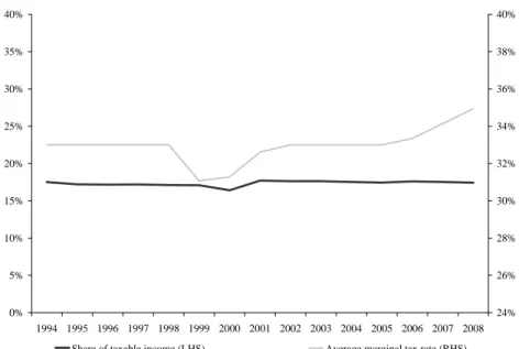
First, information about the average rates faced by different groups is summarised in Figures 3 to 5. These diagrams plot the average marginal tax rates faced by the top decile, the ninth decile and the combined eighth and seventh deciles (the fourth quintile) of income earners, along with their shares of taxable income from 1994 to 2008. Figure 3 shows that between 1994 and 2000 all top decile income earners faced a marginal tax rate of 33 per cent. Over this period their share of taxable income increased from 33.7 per cent in 1994 to 36 per cent in 1999. Following the announcement of the 39 per cent top personal rate for income above $60,000 the top decile’s share of taxable income rose sharply to 38.9 per cent in 2000. However, following the introduction of the 39 per cent rate it fell to 33.9 per cent in 2001. Between 2001 and 2008 the share of taxable income obtained by the top decilefluctuated between 33.7 per cent in 2008 and 34.6 per cent in 2005. The introduction of the 39 per cent rate led to an increase in the average marginal tax rate of the top decile. By 2006 all top decile earners faced the new top marginal rate of 39 per cent.
Figure 4 shows that over the period 1994 to 2008 those in the ninth decile of taxable income contributed, on average, 17.3 per cent to the personal income tax base. Their marginal tax rate averaged 33 per cent from 1994 to 1998 and 2002 to 2006. Between 1999 and 2001 it fell below 33 per cent for three years following a threshold and a tax rate adjustment of the middle rate. The average marginal tax rate reached 34.1 per
0% 5% 10% 15% 20% 25% 30% 35% 40% 1994 1995 1996 1997 1998 1999 2000 2001 2002 2003 2004 2005 2006 2007 2008 24% 26% 28% 30% 32% 34% 36% 38% 40%
Share of taxable income (LHS) Average marginal tax rate (RHS)
Figure 3: Top Decile Income Share and Average Marginal Tax Rate
0% 5% 10% 15% 20% 25% 30% 35% 40% 1994 1995 1996 1997 1998 1999 2000 2001 2002 2003 2004 2005 2006 2007 2008 24% 26% 28% 30% 32% 34% 36% 38% 40%
Share of taxable income (LHS) Average marginal tax rate (RHS)
0% 5% 10% 15% 20% 25% 30% 1994 1995 1996 1997 1998 1999 2000 2001 2002 2003 2004 2005 2006 2007 2008 24% 26% 28% 30% 32% 34% 36%
Share of taxable income (LHS) Average marginal tax rate (RHS)
Figure 5: Combined Seventh and Eighth Decile Income Share and Average Marginal Tax Rate
cent in 2007 and 34.9 per cent in 2008 as the number of taxpayers who moved into the top tax bracket increased.
Figure 5 shows that between 1994 and 1996 the average marginal tax rate of the seventh and eighth deciles of taxable income was around 31 per cent. However, it fell sharply to reach a low of 26.1 per cent in 2000 due to various threshold and tax rate adjustments. Since 2001 it has been rising steadily to reach 34 per cent in 2008. Over the period 2000 to 2008 these income earners experienced a slightly larger increase in their average marginal tax rate than the top decile of income earners (7.8 percentage points compared with 6 percentage points). But, in contrast to the top decile earners whose share of taxable income fell, their contribution to the personal income tax base rose slightly. It averaged 30.3 per cent between 1994 and 2000 and 31.1 per cent between 2001 and 2008.
4.2
Elasticity Estimates
The elasticities of taxable income, which compare the share of taxable income before and after the introduction of the 39 per cent rate, are reported in Table 1 for the top decile of taxable income earners. Two years are considered before the rate change. They are 1999, which pre-dates the announcement of the 39 per cent top rate and 2000, which is the year before its introduction. The elasticities are calculated for two base years because of the sharp increase in the top decile’s taxable income that occurred in 2000. Values for the ninth decile and combined seventh and eighth deciles are not reported in detail here as they were all found to be zero when using 1999 as the base year, and 0.1 when using 2000 as base year.
Table 1 reports elasticities for the top decile of between 0.4 and 1 using 1999 values as the income share before the rate change. The elasticities are substantially higher when 2000 is used as the base year for comparison, suggesting that a 1 per cent increase in the net-of-tax rate raises taxable income by 1.3 to 2.3 per cent. These values are unrealistically high, and clearly arise from the anticipation of the marginal rate increase. Hence the knowledge that a new top tax bracket is due to be introduced leads to a change in the timing of incomeflows, particularly for high income earners. This timing change is clearly reflected in Figure 3.
Table 1: Elasticity of Taxable Income in Top Decile: Introduction of 39 per cent Marginal Rate Compared with: 1999 (Pre-announcement) 2000 (Pre-introduction) 2001 1.0 2.3 2002 0.8 1.9 2003 0.9 2.0 2004 0.6 1.5 2005 0.4 1.3 2006 0.6 1.4 2007 0.7 1.5 2008 0.7 1.5
0% 5% 10% 15% 20% 25% 30% 1994 1995 1996 1997 1998 1999 2000 2001 2002 2003 2004 2005 2006 2007 2008 24% 26% 28% 30% 32% 34% 36%
Share of taxable income (LHS) Average marginal tax rate (RHS)
Figure 6: Top Percentile Income Share and Average Marginal Tax Rate
clearly more responsive to tax rate changes than lower income earners. In fact, the response of the top decile income earners is largely due to the highest earners in this group. This is illustrated by Figures 6 and 7, which plot the average marginal tax rate faced by the top percentile and the 90-99th percentiles of taxable income earners, along with their shares of taxable income from 1994 to 2008. Both taxpayer groups experi-enced an increase in their marginal tax rate. The share of taxable income remained virtually unchanged for the 90-99th percentiles. However, for the top percentile, it rose sharply in 2000, the year before the introduction of the 39 per cent rate, and then fell. Between 1994 and 2000 the top percentile of income earners contributed on average 10.2 per cent of personal income tax revenue compared with 9.3 per cent between 2001 and 2008.
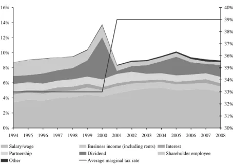
Figure 8 shows that the sharp increase in taxable income of the top percentile of income earners in 2000 was due to a rise in dividend income during that year. Under New Zealand’s imputation system, credits are attached to dividends for income tax that has been paid at the company level. The introduction of the 39 per cent top personal marginal rate and nonalignment with the company tax rate meant an additional 6 per
0% 5% 10% 15% 20% 25% 30% 35% 40% 1994 1995 1996 1997 1998 1999 2000 2001 2002 2003 2004 2005 2006 2007 2008 24% 26% 28% 30% 32% 34% 36% 38% 40%
Share of taxable income (LHS) Average marginal tax rate (RHS)
Figure 7: 90-99th Percentile Income Share and Average Marginal Tax Rate cent tax liability for earners with income above $60,000. As a result, companies paid out large profits before the 39 per cent top personal rate came into effect. Figure 8 also shows a decline in shareholder salaries following the introduction of the 39 per cent top marginal rate.
Table 2 reports the elasticities of taxable income for the top percentile of taxable income earners compared with 1999 and 2000. The elasticities of the top percentile of income earners are higher than those of the top decile earners. Values for the 90-99th percentile were found to be negligible, suggesting that most of the response of the top decile income earners is due to the top percentile earners. Again the values using 2000 as the base year are unrealistically high as a result of the bringing forward of taxable income between the announcement of the policy change and its implementation.
The difference-in-difference estimator of the elasticity of taxable income is reported in Table 3. It is the elasticity of taxable income for the top decile of income earners compared with the next decile.8 The difference-in-difference estimator produces similar
8Due to theflat income tax scales in New Zealand the top percentile versus the 90-99 percentile
of earners could not be calculated. This is because the 90-99 percentile of earners is not a meaningful control group for the top percentile of earners. Most of them, and at the end of the sample all of
0% 2% 4% 6% 8% 10% 12% 1994 1995 1996 1997 1998 1999 2000 2001 2002 2003 2004 2005 2006 2007 2008 30% 31% 32% 33% 34% 35% 36% 37% 38%
Salary/wage Business income (including rents) Interest
Partnership Dividend Shareholder employee
Other Average marginal tax rate
Figure 8: Top Percentile Income Share and Composition and Average Marginal Tax Rate
Table 2: Elasticity of Taxable Income: Top Percentile of Incomes Compared with: 1999 (Pre-announcement) 2000 (Pre-introduction) 2001 2.2 5.0 2002 1.6 4.5 2003 1.7 4.5 2004 0.9 3.7 2005 0.4 3.2 2006 1.3 4.1 2007 1.6 4.5 2008 1.8 4.6
orders of magnitude compared with the taxable income share elasticity for the top decile of taxable income earners.
Table 3: Difference-in-Difference Elasticity of Taxable Income: Top Decile versus Nineth Decile of Incomes
Compared with:
1999 (Pre-announcement) 2000 (Pre-introduction) Top Decile Incomes
2001 1.3 2.1 2002 1.2 2.0 2003 1.5 2.2 2004 1.3 1.8 2005 1.1 1.6 2006 1.0 1.6 2007 1.2 1.9 2008 1.6 2.5
It is also of interest to investigate whether females and males respond differently to marginal tax rate changes. Tables 4 and 5 report elasticities of taxable income for the top decile and for the top percentile of income earners.9 Values for lower deciles are
negligible, as are the values for the 90-99th percentiles, and are thus not reported. The results confirm the previous finding that higher income earners are more responsive to marginal tax rate changes than lower income earners for both females and males. The elasticity estimates for the top percentile income earners exceeds that of the top decile. Moreover, the results suggest that men may be more responsive than women to tax rate changes, when 1999 is used as the base year, thereby avoiding the income shifting between periods, discussed above. Women are likely to be less responsive to tax rate changes than men because they have lower incomes. This can be seen in Figure 9, which plots the average income of the top decile female and male earners for 1994 to 2008. The average income of the top decile female earners rose steadily from $48,983 in 1994 to $83,237 in 2008. By comparison, the top decile of male incomes increased
them, faced the same marginal tax rate as the top percentile of earners.
9Elasticities of the top decile compared with the ninth decile are not reported here, because the
relatively higher increase in incomes of females in the ninth decile impart a large downward bias. Values for males steadily increase from 0.8 in 2001 to 1.8 in 2007, when 1999 is the base year.
Compared with:
1999 (Pre-announcement) 2000 (Pre-introduction)
Female Male Female Male
Top Decile Incomes
2001 0.6 0.9 2.7 1.9 2002 0.2 0.7 2.0 1.7 2003 0.5 0.8 2.2 1.8 2004 0.3 0.6 1.7 1.5 2005 0.2 0.5 1.4 1.4 2006 -0.2 0.8 0.8 1.8 2007 0.1 0.9 1.0 1.8 2008 0.3 0.9 1.1 1.8
Table 5: Elasticity of Taxable Income: Top Percentile of Incomes Compared with:
1999 (Pre-announcement) 2000 (Pre-introduction)
Female Male Female Male
Top Percentile Incomes
2001 1.5 2.5 4.0 5.6 2002 1.2 1.8 3.7 4.8 2003 1.0 1.8 3.6 4.9 2004 1.0 0.6 3.5 3.7 2005 0.7 0.0 3.2 3.0 2006 -0.4 2.0 2.1 5.0 2007 0.6 2.0 3.1 5.1 2008 1.2 1.8 3.7 4.9
48,983 50,29553,299 55,837 57,27960,614 67,212 62,01465,466 66,780 70,77873,681 78,848 80,59783,237 85,070 92,175 94,33398,074 101,418 110,299 100,997 107,461 117,897 125,204 128,895 135,501 108,962 122,872 129,338 0 20,000 40,000 60,000 80,000 100,000 120,000 140,000 160,000 1994 1995 1996 1997 1998 1999 2000 2001 2002 2003 2004 2005 2006 2007 2008 Females Males
Figure 9: Average Incomes of Top Decile of Female and Male Earners
from $85,070 to $135,501. Also notable is the increase in the average taxable income of male earners from $110,299 in 1999 to $129,338 in 2000 and the drop in 2001 to $100,997.
5
Empirical Results: Fiscal Drag
This section reports estimates of taxpayers’ responsiveness to changes in marginal tax rates by examining the behaviour of earners, whose marginal tax rate increased because they moved into a higher tax bracket as a result of fiscal drag. The period 2001 to 2008 is considered, as during this time no threshold or marginal rate changes were made to the lower income tax brackets. Elasticities of taxable income are derived for all taxpayers and for females and males separately.
The effects of fiscal drag can be examined by using the difference-in-difference es-timator in (7). In previous studies this has, for example, been used by taking as the control group those individuals within a tax bracket who remain in the same bracket from one period to the next, despite a general upward movement in incomes. The
treat-bracket and thus experience an increase in their marginal tax rate. The denominator of (7), as a proportionate difference in net-of-tax rates, is negative. The numerator is expected also to be negative, since those people moving into a higher tax bracket (consisting mainly of those who were near the top of the initial tax bracket), are likely to respond to the higher tax rate by modifying the increase in their declared taxable income. This situation arises where all those in the tax bracket would experience sim-ilar rates of income growth over the time period, if there were no tax consequences. Thus it is assumed that there are no systematic non-tax-related income changes.
However, in the present context, it was found that there are significant variations in income movements. For example, there are many individuals who move from the second highest tax bracket, often into a lower tax bracket, while others move into the highest income range. This type of income dynamics produces a substantial bias if (7) is directly applied. Hence the following approach was used instead.
The calculations are based on people who were in the same tax bracket in period, where some of those taxpayers moved into a higher income tax bracket in period+ 1. The difference-in-difference elasticity compares the change in taxable income of these income recipients between periods+ 1 and+ 2. Taxable income may have changed because taxpayers adjusted how much they work or save, because of tax planning or because they exited paid market employment or emigrated from New Zealand and hence dropped out of the sample.
The elasticities of earners who moved into the top bracket and of taxpayers who moved into the second highest tax bracket are reported in Table 6. The results confirm earlier findings that higher income earners are more responsive than lower income taxpayers. The elasticities of people who moved into the top bracket are higher than those of taxpayers who moved into the second highest tax bracket. But the elasticities of earners who moved into the top bracket are lower than those of the top decile of earners reported in Table 3.
Consider next the question of whether higher and lower income earners respond differently at the intensive and extensive margin to changes in their marginal tax
Table 6: Elasticity of Taxable Income: Earners Moving into the Top and the Second Highest Bracket
Earners Moving into the:
Highest Bracket Second Highest Bracket
2002 0.5 0.2 2003 1.7 0.0 2004 1.3 0.3 2005 1.1 0.2 2006 0.8 0.1 2007 0.9 0.1 2008 0.7 0.2
rates. International evidence suggests that higher income earners tend to respond at the intensive margin; that is they adjust their taxable income by changing work effort, hours worked, the amount they save, and so on. However, lower income earners and secondary earners tend to respond at the extensive margin; that is, they often leave or enter the labour market in response to an increase or decrease in their marginal tax rate.
Figure 10 plots the elasticities of taxable income of all earners who moved into the top tax bracket and the elasticities of earners who moved into the top bracket but excluding taxpayers who exited the sample. The figure shows that overall the elasticities are similar; that is, people do not seem to exit paid market employment when they move into the top tax bracket.
However, a different picture emerges for lower income taxpayers. Figure 11 plots the elasticities of taxable income of all earners who moved into the second highest bracket and the corresponding elasticities, excluding taxpayers who exited the sample. It shows that the values obtained by excluding taxpayers who exited the sample are consistently higher than those for all income recipients. This finding suggests, in line with international evidence, that lower income taxpayers who experience an increase in their marginal tax rate are more likely to exit paid market employment than higher income earners whose marginal tax rate increases.
be-0.0 0.2 0.4 0.6 0.8 1.0 1.2 1.4 1.6 2002 2003 2004 2005 2006 2007 2008 Elasticity of taxable income of all earners Elasticity of taxable income excluding earners who exited the sample
Figure 10: Revenue Elasticity of Earners Moving into the Top Bracket — All Earners and Excluding Those Who Exited the Sample
0.0 0.1 0.1 0.2 0.2 0.3 0.3 0.4 2002 2003 2004 2005 2006 2007 2008 Elasticity of taxable income of all earners Elasticity of taxable income excluding earners who exited the sample
Figure 11: Revenue Elasticity of Earners Moving into the Second Highest Bracket — All Earners and Excluding Those Who Exited the Sample
cause they moved into the top tax bracket, are summarised in Table 7 for all taxpayers and excluding those who exited the sample. Once again, male earners tend to have higher elasticities than female earners. But neither men nor women appear to be more likely to exit paid market employment or emigrate from New Zealand when moving into the top bracket.
At lower incomes, however, women appear to be more responsive to changes in their marginal tax rates than men both at the intensive and extensive margin. This is shown in Table 8, which reports the elasticities of taxable income of female and male earners who moved into the second highest tax bracket for all earners and excluding taxpayers who left the sample. Both elasticities are higher for women than men in all years except for 2008 when the elasticity excluding people who left the sample was higher for male earners compared with female earners. The downward bias resulting from not excluding those who left the sample is clear, especially for men in this bracket.
Table 7: Elasticity of Taxable Income: Earners Moving into the Top Bracket Including all earners Excluding those who
left the Sample Female Male Female Male
2002 -0.5 1.1 0.8 1.1 2003 2.2 1.5 1.6 1.4 2004 1.0 1.5 1.2 1.2 2005 0.7 1.3 0.8 1.0 2006 1.4 0.6 1.2 0.8 2007 0.5 1.2 0.5 0.9 2008 0.7 0.8 0.6 0.8
6
Some Comparisons
Many empirical estimates of the elasticity of taxable income have been produced for a large range of countries, as discussed by, for example, Saez et al. (2009). The values vary considerably, depending on the method of estimation used, the particular reform examined, and the country. After mentioning that a number of authors suggest a
Including all earners Excluding those who left the sample Female Male Female Male
2002 0.3 0.0 0.4 0.1 2003 0.2 -0.1 0.3 0.3 2004 0.4 0.1 0.4 0.2 2005 0.2 0.1 0.2 0.2 2006 0.2 -0.1 0.3 0.1 2007 0.2 -0.1 0.2 0.2 2008 0.3 0.0 0.2 0.3
‘consensus value of about 0.4’, Giertz (2004, pp. 14, 37) warns that this ‘masks con-siderable variation in the estimates’. Indeed, there is no reason to expect the elasticity to remain unchanged over time, or to be similar across countries having different tax structures and regulations. Furthermore, the above results have demonstrated some heterogeneity among types of taxpayer, so that there seems little value in attempting tofind a consensus value.
Another feature of many estimates is that much uncertainty is attached to them, in that they have wide confidence intervals. After reviewing elasticities, Meghir and Richards (2007, p. 19) comment that ‘the estimates of the effect of taxes on taxable income, whose purpose is to identify the impact of taxation on other dimensions of effort, should be regarded with caution’. Furthermore, Saezet al. (2009, p. 59) suggest that, ‘there are no convincing estimates of the long-run elasticity’. The suggestion, by Saezet al. (2009) that some ‘short run’ elasticity estimates obtained from tax reforms may perhaps capture changes in the timing of declarations, has been confirmed by the above analysis of the introduction of the 39 per cent tax rate in New Zealand.
The use of a ‘reduced form’ specification inevitably carries with it the difficulty that, when a parameter estimate is found to change from one dataset to another, there is no way of knowing precisely what has caused the change. It has been demonstrated above that examination of the various income components is important, particularly among the higher income taxpayers. Giertz (2004, p. 39) suggested that, ‘much work
is still needed in order to better understand the process by which incomes respond to changes’. This judgement was repeated by Saezet al. (2009) who stressed the need to look at the various margins involved in responses to taxation. The value of examining the different margins was indeed demonstrated in the previous section.
Where it has been possible to estimate elasticities for different income ranges, a common result is that they vary with income, being higher for higher incomes. This result has been confirmed by the present analysis, and it is perhaps not surprising in view of the fact that higher income groups may be expected to have more opportunities to shift income between sources.
Faced with the difficulty of obtaining data in New Zealand, there is only one pre-vious study containing estimates of the elasticity of taxable income for New Zealand. Using a variety of methods, covering a number of tax structure changes, Thomas (2007, p. 22) obtained estimates which ‘ranged from 0.35 to 1.10, with a preferred estimate of 0.52’; see also Thomas (2007, p. 18). The present results are thus broadly in line with those reported by Thomas. He found that the tax rate reductions in the mid-1980s produced substantial reductions in the excess burden from income taxation. Similarly, the increase in the top marginal rate in 2001 again raised excess burdens, though to levels below those of the 1980s. He reported marginal welfare costs of as high as $8 per extra dollar of revenue raised. The following Section truns to the measurement of such welfare costs.
7
Marginal Welfare Costs
This section considers the efficiency costs of personal income taxation. Subsection 7.1 shows how marginal welfare costs of the top marginal tax rate can be obtained using the elasticity of taxable income concept, under a range of assumptions, in particular the absence of income effects. Appendix B extends the method to deal with all tax brackets and also provides information about the relevant income distribution terms and other components required for obtaining the marginal welfare cost. Subsection 7.2 reports empirical results.
This subsection considers the efficiency effects of changes in the top marginal income tax rate in a multi-rate system. This has received most attention in the literature and is the policy change considered in Section 4. Suppose income above the threshold, ,
is taxed at thefixed rate,. If this is the top marginal rate, so that there are no income thresholds above , the tax paid at that rate by an individual is given, for ,
by(−) and total revenue collected by the top marginal rate, , is thus:
= X
(−) =(¯ −) (8)
where ¯ is the arithmetic mean of those above the threshold, and is the number
of people whose taxable income is above the threshold. It is important to recognise that(−)is not the total tax paid by person, since the latter has to include tax
paid at lower rates. However, changes in the top rate are of course expected to have no effect on revenue from the lower rates.
The effect on , and thus on total revenue, of a change in is thus:
= + ¯ ¯ (9)
The first term is a pure ‘tax rate’ effect while the second term is a ‘tax base’ effect of the tax rate change. Using = (¯ −), ¯ =, and from the definition
of , ¯ =−1−¯, the revenue change becomes:10
=(¯ −) ½ 1− µ ¯ ¯ − ¶ µ 1− ¶¾ (10) Let(), ()and1() = 0 () ∞
0 () denote the density function, the distribution function and the first moment distribution function of . The Lorenz curve is, for example, the relationship between ()and1(), the proportion of people associated
with a proportion of total income (cumulating from lowest to highest). In general it can be shown that:
¯ ¯ − = ∙ 1−³ ¯ ´ 1− () 1−1() ¸−1 (11) 10This is equivalent to the result stated by Saezet al. (2009, p. 5, equation 5).
where¯is the arithmetic mean of the complete distribution of . Define: = ¯ ¯ − (12) so that (10) is more succinctly written as:
=(¯ −) ½ 1− µ 1− ¶¾ (13) The tax rate, ∗, which maximises revenue from the top marginal rate, obtained by
setting = 0, is thus a simple function of and the elasticity, , whereby:
∗ = (1 +)−1 (14)
The revenue change in (10) depends on the precise form of the distribution of declared income and the income threshold above which the tax rate of applies. The various components of (11) can be obtained from information about the distribution of declared incomes.
The marginal welfare cost, , defined as the marginal excess burden divided by the change in tax revenue, is:11
=
1− −
(15) This expression is relevant only when the marginal tax rate is below the revenue-maximising rate in (14), so that 0.12 The extension to cover all tax brackets is
given in Appendix B.
7.2
Empirical Results
The results of the previous section, along with Appendix B, enable the marginal welfare cost to be evaluated for any tax bracket, given cross-sectional information about the 11Saezet al. (2009, p. 6) call the the ‘marginal efficiency cost of funds (MECF)’. However,
the ‘marginal cost of funds’, or , is usually defined as1 + . On these concepts, see Creedy (1998, pp. 54-59).
12Suppose a proportion,, of the reduction in declared income attracts a tax rate of . Saezet
al. (2009, p. 9) show that =(¯−)
n
1−³1−−´oand =1−−(−(−)). Again this is relevant only for parameter values for which
0, that is for values of which are less than∗,
given by∗=1+
Earlier results have produced a range of values for the elasticity, with lower values in lower income groups and for women compared with men (with the exception of the fiscal drag results for movement into the second highest tax bracket). For this reason computations were carried out for a range of values of in each tax bracket, thereby also enabling the sensitivity of welfare changes to to be examined.
Tables 9 and 10 report the marginal welfare costs for each year and tax bracket, for four alternative values of. A dash in any cell of the table indicates that the tax rate exceeds the revenue-maximising rate for that tax bracket. This occurs in a substantial number of cases, particularly for the top marginal rate groups and the higher elasticity values. The estimates reported above are indeed in those higher ranges. As expected the marginal welfare costs for the lower elasticity values and the lower tax brackets are relatively small, while for the top tax bracket they are large — mostly in excess of unity.13 Thus for those top brackets, when the tax rate is below the revenue-maximising
value, the welfare cost of raising an extra dollar of revenue is well in excess of a dollar. Furthermore, it can be seen that the welfare costs for the top marginal rate bracket increase substantially after the introduction of the 39 per cent top tax rate. To the extent that a proportion of taxable income is being diverted into other sources which attract lower tax rates, the above estimates overstate the marginal welfare costs, as discussed in footnote 12 above. Insufficient information is available, about the diverted proportions and associated rates, on which to base an adjustment here.
It is known that the marginal welfare costs can be highly sensitive with respect to the elasticity of taxable income. However, the values reported in these two tables are relatively stable in the lower and middle tax brackets, becoming more sensitive for the higher marginal rates. For the lower tax brackets, where the rates and thresholds remain stable, the welfare costs change very little over time, reflecting the relative stability in the distribution of taxable incomes.
13Higher welfare costs for individuals in Australia were found by Creedy et al. (2008), using a
structural labour supply model, even though labour supply changes were small. The assumption of zero income effects which is imposed in the present analysis may thus affect results.
Table 9: Marginal Welfare Costs Threshold = 05 = 07 = 09 = 11 1994 0 0.15 0.04 0.06 0.07 0.09 9501 0.28 0.17 0.26 0.35 0.47 30875 0.33 1.51 5.3 - -1995 0 0.15 0.04 0.06 0.07 0.09 9501 0.28 0.18 0.27 0.37 0.49 30875 0.33 1.37 4.27 - -1996 0 0.15 0.04 0.06 0.07 0.09 9501 0.28 0.18 0.27 0.38 0.5 30875 0.33 1.36 4.18 - -1997 0 0.15 0.04 0.05 0.07 0.09 9501 0.25 0.16 0.24 0.33 0.44 30876 0.2625 - - - -34200 0.33 1.4 4.47 - -1998 0 0.15 0.04 0.05 0.07 0.09 9501 0.24 0.14 0.21 0.29 0.38 34200 0.33 1.36 4.18 - -1999 0 0.15 0.04 0.05 0.07 0.09 9501 0.2175 0.12 0.18 0.25 0.32 34201 0.24 0 0 0 0 38000 0.33 1.27 3.6 0 0 2000 0 0.15 0.04 0.06 0.07 0.09 9501 0.21 0.11 0.17 0.22 0.29 38000 0.33 1.03 2.45 10.52 -2001 0 0.15 0.04 0.05 0.07 0.09 9501 0.21 0.11 0.16 0.21 0.27 38001 0.33 - - - -60000 0.39 4.32 - -
-Threshold = 05 = 07 = 09 = 11 2002 0 0.15 0.04 0.05 0.07 0.09 9501 0.21 0.11 0.16 0.21 0.28 38001 0.33 - - - -60000 0.39 3.83 - - -2003 0 0.15 0.04 0.05 0.07 0.08 9501 0.21 0.11 0.16 0.22 0.28 38001 0.33 - - - -60000 0.39 3.98 - - -2004 0 0.15 0.04 0.05 0.07 0.08 9501 0.21 0.11 0.16 0.22 0.28 38001 0.33 - - - -60000 0.39 3.55 - - -2005 0 0.15 0.04 0.05 0.07 0.09 9501 0.21 0.11 0.16 0.22 0.28 38001 0.33 - - - -60000 0.39 3.3 - - -2006 0 0.15 0.04 0.05 0.07 0.09 9501 0.21 0.11 0.16 0.21 0.27 38001 0.33 - - - -60000 0.39 3.9 - - -2007 0 0.15 0.04 0.05 0.07 0.09 9501 0.21 0.11 0.16 0.21 0.27 38001 0.33 - - - -60000 0.39 4.14 - - -2008 0 0.15 0.04 0.05 0.07 0.09 9501 0.21 0.11 0.16 0.21 0.27 38001 0.33 - - - -60000 0.39 4.14 - -
-8
Conclusions
This paper has provided estimates for New Zealand of the concept of the elasticity of taxable income, with respect to changes in the net-of-tax marginal tax rate. This con-cept has the advantage of measuring, in a reduced-form context, all possible responses to tax rate changes and of enabling the efficiency effects to be measured. Results were obtained using a special dataset constructed from a random sample of New Zealand taxpayers.
Two approaches were used to estimate elasticity values for different groups of tax-payers. First, the introduction of an additional top marginal tax rate bracket provided a useful policy change as a natural experiment. Secondly, the stability of the tax struc-ture over recent years enables the effect offiscal drag, in shifting some individuals into a higher marginal tax rate bracket, to be considered. In using the first approach, it was particularly important to consider the possibility that some observed responses to tax changes may involve the timing, rather than the total amount, of taxable income declared, particularly in anticipation of announced changes taking effect. Furthermore, in estimating the elasticity, care needs to be taken to avoid attributing some of the changes in declared income to marginal tax changes, when they may have arisen from other dynamic factors. Non-tax-related income movements were observed, particularly when attempting to base estimates on tax rate changes arising fromfiscal drag and the movement into higher tax brackets.
In view of these complications, the results should be treated with caution. Never-theless, it was found that the elasticity of taxable income is substantially higher for the highest income groups. Indeed for lower deciles of the income distribution, the elasticity was found to be negligible. Generally the elasticity was higher for men than for women. This may be largely because the taxable incomes of men are systemat-ically above those of women. Changes in the timing of income flows for the higher income recipients was found to be an important response to the announcement of a new higher-rate bracket. The marginal welfare costs of personal income taxation were consistent across years, being relatively small for all but the higher tax brackets. For
of tax revenue was found to be well in excess of a dollar. Furthermore, for the top bracket the marginal tax rate was often found to exceed the revenue-maximising tax rate, for appropriate values of the elasticity of taxable income.
Appendix A: The Data
This appendix describes the data used in the analysis. The database was constructed by randomly sampling Inland Revenue’s individual taxpayer population. It covers the period from 1994 to 2008. The random sample is weighted to match the total population. The database includes people with wage/salary income (including taxable welfare benefits) and people who filed an IR5 or IR3 tax return or received a personal tax summary (PTS). It excludes people with no personal taxable income unless they filed.
The requirement for wage and salary earners tofile an IR5 tax return was in part based on earnings over a threshold. This threshold was eased during the 1990s from $20,000 in the early 1990s, to $38,000 by 1999. However a significant administrative change in 2000 removed the IR5 tax return entirely and replaced it with the PTS, a pre-populated taxpayer square-up based on data collected from employers during the year. The income threshold was removed, with a consequential reduction in the number of taxpayers required to square-up. This has caused a structural break in the income tax data collected, especially on dividend and interest income. Taxpayers who previously filed an IR5 were not required to square up via a PTS if their only income was from salary and wages or from investments with the correct amount of tax deducted at source, or where the investment income was below a certain threshold.
Individual taxpayer information is gathered from the following sources/returns: 1. Client registration
2. Individual tax return IR3
3. Personal tax summary (PTS) from 2000 onwards
4. Salary/wage earner income tax return IR5 (pre-PTS) from 1994 to 1999 5. Employer monthly schedule (EMS) from 2000 onwards
taxpayer’s ‘entity class’; a client registration feature: (a) salary/wage earner with a salary/wage (SW) entity class; and (b) other taxpayers with a non-SW entity class (for example, self-employed or salary/wage earners with other income from rental properties or overseas investments). The selection method is as follows:
1. A random two per cent of total salary/wage earners — with the random sample selected from the last two digits of their IRD number;
2. A random ten per cent of total other individual taxpayers — also based on the last two digits of the IRD number with the chosen range including the two per cent sample above.
A taxpayer generally has one IRD number and the same entity class. However, a minority of taxpayers could have a second IRD number due to bankruptcy or they might retain the same IRD number but change entity class over time. This means that the above selection method will have some ‘missing’ taxpayers if a taxpayer has an entity class change from non-SW to SW, or a taxpayer is issued a new IRD number because of bankruptcy.
Variables The dataset contains the following main variables: 1. General variables — unique IRD number, date of birth, gender
2. Income variables — salary/wage earning, business income, estate or trust benefi -ciary income, interest income, dividend income, overseas income, rental income, shareholder-employee salary, partnership income, other income, taxable income 3. Other variables — expenses, losses claimed, loss attributing qualifying company
(LAQC) losses claimed
The gender variable is determined based on the ‘title’ of a taxpayer (e.g. Mr and Miss) so some imputation is required. When no title is present, or the title is ambiguous, gender is randomly assigned.
Some of the variables are unique to IR3 filers and not available for non-filers. Dif-ferences in the returnfinancial variables are summarised in Table 11:
Table 11: Income Variables
IR3 PTS/IR5 Non filer TDC/EMS
Salary/wage income Salary/wage income Salary/wage earning Interest income Interest income
Dividend income Dividend income Business income
Estate or trust beneficiary income Overseas income
Shareholder-employee salary Net rents
Partnership income Other income
LAQC losses claimed Expenses
Losses claimed Taxable income
Taxable income is the sum of all incomes less LAQC losses claimed, less expenses and less losses claimed (in that order). Taxable income is zero if a taxpayer has negative taxable income (i.e. a loss). As the focus is on income, rebates (such as child care, housekeeping and donations) are ignored.
The expenses variable is different from the business expenses that can be claimed in the general set of financial accounts. The expenses variable can be defined as ‘fees’ paid for professional services:
• A fee to someone for completing a tax return
• Commission on interest or dividend income
• Expenses incurred in earning income that has had withholding tax deducted
• Additional expenses incurred in earning partnership income, for example, interest on capital borrowed to purchase a share in the partnership
• Premiums on loss of earnings insurance (income protection), provided the benefit from the insurance policy is taxable
Appendix B: Welfare Costs for all Income Tax
Brack-ets
This appendix shows how marginal welfare costs can be obtained for any tax bracket in a multi-rate system. Suppose that in the th tax bracket the marginal tax rate is above the income threshold , for = 1 . For +1 the tax paid
at the rate is simply (−), and for +1 the tax paid at that rate is
(+1−). Hence if ()denotes the distribution function of taxable income, the
total tax paid at the rate, denoted, is given by:
= Z +1 (−)() +(+1−) Z ∞ +1 () (B.1) Expanding terms, and letting 1() denote the first moment distribution function of
, and the total population size:
=[¯{1(+1)−1()}−{(+1)− ()} + (+1−){1− (+1)}]
(B.2) where ¯ is the arithmetic mean of the complete distribution of . The number of individuals with income in theth tax bracket, , is:
={ (+1)− ()} (B.3)
The number of people with income above the threshold+1, that is, the number above
theth tax bracket, ++1, is:
++1 ={1− (+1)} (B.4)
Furthermore, if¯ denotes the arithmetic mean of within the th tax bracket, then: ¯ = ¯ {1(+1)−1()} { (+1)− ()} (B.5) Thus revenue raised by the th rate is:
= + ¯ ¯ (B.7) Thefirst term is the pure ‘tax rate’ effect while the second term is the ‘tax base’ effect of the tax rate change. Here:
=(¯−) +++1(+1−) (B.8)
Furthermore, ¯
=, and if the elasticity of taxable income in the th bracket is
: ¯ =− ¯ 1− (B.9) The revenue change thus becomes:
=(¯−) ½ 1− µ ¯ ¯ − ¶ µ 1− ¶¾ +++1(+1−) (B.10)
In considering the welfare change, allowance must be made for the income change of those above the threshold, +1, though they do not experience a change in their
effective marginal tax rate and there is no excess burden. For those with +1,
the welfare change is, as obtained above, given by −. Thus, writing= (¯¯−),
aggregate marginal excess burden, , is similar to the earlier result that: =(¯−)
1−
(B.11) However, the marginal welfare cost becomes:
= 1−−+ (B.12) where: = ++1 µ +1− ¯ − ¶ (1−) (B.13)
and substitution gives: =
(1−) (+1−){1− (+1)}
¯
{1(+1)−1()}−{(+1)− ()}
The result for the top marginal rate is thus simply the special case where +1 = ∞
and (+1) = 1(+1) = 1, so that = 0. If, as for example in New Zealand,
there is no tax-free threshold in the income tax structure, so that 1 = 0, it can be
seen that 1 = 1 and 1 = [(1−1{)¯21{(1−2)}(2)}].
Tables 12 and 13 report the various components — other than the elasticity of taxable income — needed to compute the welfare measures. The tax rates, , in Tables 12 and
Thresholds ¯ 1994 0-9,500 15 1.00 1.12 4,868 9,501-30,875 28 2.16 1.36 17,690 Over 30,875 33 2.44 0.00 52,293 1995 0-9,500 15 1.00 1.13 4,777 9,501-30,875 28 2.15 1.28 17,766 Over 30,875 33 2.35 0.00 53,819 1996 0-9,500 15 1.00 1.14 4,656 9,501-30,875 28 2.13 1.24 17,894 Over 30,875 33 2.34 0.00 54,002 1997 (composite year) 0-9,500 15 1.00 1.23 4,331 9,501-30,875 25 2.19 1.22 17,457 30,876-34,200 26.25 19.84 -1.45 32,515 Over 34,200 33 2.37 0.00 59,187 1998 0-9,500 15 1.00 1.25 4,206 9,501-34,200 24 2.03 1.19 18,682 Over 34,200 33 2.34 0.00 59,768 1999 (composite year) 0-9,500 15 1.00 1.18 4,432 9,501-34,200 21.75 2.05 1.24 18,550 34,201-38,000 24 19.08 -1.29 36,092 Over 38,000 33 2.27 0.00 67,866 2000 0-9,500 15 1.00 1.12 4,409 9,501-38,000 21 1.91 1.18 19,905 Over 38,000 33 2.06 0.00 73,945
Table 13: Marginal Welfare Cost Components: 2001—2008 Thresholds ¯ 2001 2002 0-9,500 15 1.00 1.20 4,260 1.00 1.22 3,980 9,501-38,000 21 1.90 1.26 20,108 1.89 1.23 20,214 38,001-60,000 33 5.24 -0.60 46,970 5.19 -0.67 47,080 Over 60,000 39 2.54 0.00 98,871 2.48 0.00 100,475 2003 2004 0-9,500 15 1.00 1.28 3,708 1.00 1.26 3,620 9,501-38,000 21 1.89 1.19 20,209 1.87 1.18 20,405 38,001-60,000 33 5.13 -0.68 47,200 5.11 -0.80 47,248 Over 60,000 39 2.50 0.00 100,014 2.44 0.00 101,562 2005 2006 0-9,500 15 1.00 1.22 3,528 1.00 1.19 3,434 9,501-38,000 21 1.85 1.18 20,617 1.84 1.21 20,786 38,001-60,000 33 5.07 -0.92 47,341 5.02 -1.00 47,460 Over 60,000 39 2.40 0.00 102,977 2.49 0.00 100,321 2007 2008 0-9,500 15 1.00 1.20 3,550 1.00 1.19 3,479 9,501-38,000 21 1.83 1.19 20,966 1.81 1.18 21,239 38,001-60,000 33 5.00 -1.18 47,499 4.93 -1.42 47,676 Over 60,000 39 2.52 0.00 99,381 2.52 0.00 99,466
This appendix provides summary information on the number and percentage of tax-payers by income and the sum and percentage of taxable income by income band.
Table 14: Taxable Incomes by Income Band: 1994—1998
1994 1995 1996 1997 1998
Number of Taxpayers by Income Band
0-9,000 829,840 758,388 742,790 725,388 717,600 9,001-38,000 1,571,680 1,660,907 1,672,044 1,702,448 1,704,142 38,001-60,000 255,160 263,632 288,742 313,405 329,214 Over 60,000 104,320 119,043 132,356 146,923 156,408 Total 2,761,000 2,801,970 2,835,932 2,888,164 2,907,364
Percentage of Taxpayers by Income Band
0-9,000 30 27 26 25 25
9,001-38,000 57 59 59 59 59
38,001-60,000 9 9 10 11 11
Over 60,000 4 4 5 5 5
Total 100 100 100 100 100
Sum of Taxable Income by Income Band (dollar million)
0-9,000 3,748 3,124 2,987 2,841 2,796
9,001-38,000 30,582 32,037 32,761 33,245 33,541 38,001-60,000 11,744 12,155 13,335 14,498 15,266 Over 60,000 10,738 12,648 13,936 15,521 16,672
Total 56,812 59,964 63,020 66,104 68,275
Percentage of Taxable Income by Income Band
0-9,000 7 5 5 4 4
9,001-38,000 54 53 52 50 49
38,001-60,000 21 20 21 22 22
Over 60,000 19 21 22 23 24
Table 15: Taxable Incomes by Income Band: 1999—2003
1999 2000 2001 2002 2003
Number of Taxpayers by Income Band
0-9,000 689,783 692,240 704,370 698,960 689,490 9,001-38,000 1,681,660 1,699,910 1,715,080 1,718,650 1,735,260 38,001-60,000 341,990 357,870 399,100 437,230 470,910 Over 60,000 173,585 187,560 193,550 221,251 236,661 Total 2,887,018 2,937,580 3,012,100 3,076,091 3,132,321
Percentage of Taxpayers by Income Band
0-9,000 24 24 23 23 22
9,001-38,000 58 58 57 56 55
38,001-60,000 12 12 13 14 15
Over 60,000 6 6 6 7 8
Total 100 100 100 100 100
Sum of Taxable Income by Income Band (dollar million)
0-9,000 2,647 2,613 2,593 2,457 2,368
9,001-38,000 32,538 32,881 33,604 34,084 34,700 38,001-60,000 15,881 16,648 18,748 20,588 22,230 Over 60,000 19,111 23,685 19,139 22,238 23,676
Total 70,178 75,828 74,085 79,367 82,974
Percentage of Taxable Income by Income Band
0-9,000 4 3 4 3 3
9,001-38,000 46 43 45 43 42
38,001-60,000 23 22 25 26 27
Over 60,000 27 31 26 28 29
2004 2005 2006 2007 2008 Number of Taxpayers by Income Band
0-9,000 686,000 692,670 706,130 677,140 651,920 9,001-38,000 1,718,580 1,712,800 1,694,770 1,674,030 1,668,720 38,001-60,000 509,780 547,840 582,430 614,790 649,690 Over 60,000 277,141 312,971 352,881 400,711 453,091 Total 3,191,501 3,266,281 3,336,211 3,366,671 3,423,421
Percentage of Taxpayers by Income Band
0-9,000 21 21 21 20 19
9,001-38,000 54 52 51 50 49
38,001-60,000 16 17 17 18 19
Over 60,000 9 10 11 12 13
Total 100 100 100 100 100
Sum of Taxable Income by Income Band (dollar million)
0-9,000 2,339 2,288 2,277 2,261 2,066
9,001-38,000 34,787 35,007 34,937 34,807 35,018 38,001-60,000 24,089 25,938 27,645 29,204 30,977 Over 60,000 28,151 32,233 35,406 39,826 45,071 Total 89,367 95,466 100,265 106,099 113,131
Percentage of Taxable Income by Income Band
0-9,000 3 2 2 2 2
9,001-38,000 39 37 35 33 31
38,001-60,000 27 27 28 28 27
Over 60,000 32 34 35 38 40
References
[1] Creedy, J. (1998) Measuring Welfare Changes and Tax Burdens. Cheltenham: Edward Elgar.
[2] Creedy, J. (2009) The elasticity of taxable income: an introduction. University of Melbourne Department of Economics Working Paper, no. 1085.
[3] Creedy, J., Hérault, N. and Kalb, G. (2008) Comparing welfare change measures with income change measures in behavioural microsimulation.University of Mel-bourne Department of Economics Working Paper, no. 1030.
[4] Evans, L., Grimes, A., Wilkinson, B. and Teece, D.(1996) Economic reform in New Zealand 1984-95: the pursuit of efficiency. Journal of Economic Literature, 34, pp. 1856-1902.
[5] Feldstein, M. (1995) The effect of marginal tax rates on taxable income: a panel study of the 1986 Tax Reform Act.Journal of Political Economy, 103, pp. 551-572. [6] Giertz, S.H. (2004) Recent literature on taxable income elasticities. Tax Analysis
Division Congressional Budget Office, Washington D.C., paper 2004-16.
[7] Meghir, C. and Phillips, D. (2007) Labour supply and taxes. Institute for Fiscal Studies.
[8] Onrubia, J. and Sanz, J.F. (2009) Reported taxable income and marginal tax rates: evidence for Spain based onfiscal drag.Universidad Complutense de Madrid Working Paper.
[9] Saez, E., Slemrod, J.B. and Giertz, S.H. (2009) The elasticity of taxable income with respect to marginal tax rates: a critical review.National Bureau of Economic Research Working Paper, no. 15012.
[10] Thomas, A. (2007) Taxable income elasticities and the deadweight cost of taxation in New Zealand. Unpublished paper, Inland Revenue, Wellington.