PARALLEL SPARQL QUERY EXECUTION
USING APACHE SPARK
A THESIS IN Computer Science
Presented to the Faculty of the University of Missouri-Kansas City in partial fulfillment
of the requirements for the degree MASTER OF SCIENCE
by
HASTIMAL JANGID B.TECH, WBUT Kolkata, 2010
Kansas City, Missouri 2016
© 2016
HASTIMAL JANGID ALL RIGHTS RESERVED
iv
PARALLEL SPARQL QUERY EXECUTION
USING APACHE SPARK
Hastimal Jangid, Candidate for the Master of Science Degree University of Missouri-Kansas City, 2016
ABSTRACT
Semantic Web technologies such as Resource Description Framework (RDF) and SPARQL are increasingly being adopted by applications on the Web, as well as in domains such as healthcare, finance, and national security and intelligence. While we have witnessed an era of many different techniques for RDF indexing and SPARQL query processing, the rapid growth in the size of RDF knowledge bases demands scalable techniques that can leverage the power of cluster computing. Big data ecosystems like Apache Spark provide new opportunities for designing scalable RDF indexing and query processing techniques.
In this thesis, we present new ideas on storing, indexing, and query processing of RDF datasets with billions of RDF statements. In our approach, we will leverage Resilient Distributed Datasets (RDDs) and MapReduce in Spark and the graph processing capability of GraphX. The key idea is to partition the RDF dataset, build indexes on the partitions, and execute a query in parallel on the collection of indexes. A key theme of our design is to enable in-memory processing of the indexes for fast query processing.
v
APPROVAL PAGE
The faculty listed below, appointed by the Dean of the School of Computing and Engineering, have examined a thesis titled “Parallel SPARQL Query Execution Using Apache Spark”, presented by Hastimal Jangid, candidate for the Master of Science degree, and certify that in their opinion, it is worthy of acceptance.
Supervisory Committee
Praveen Rao, Ph.D. Committee Chair School of Computing and Engineering, UMKC
Zhu Li, Ph.D. Committee Member School of Computing and Engineering, UMKC
Geetha Manjunath, Ph.D., Committee Member Research Lab Manager, Xerox Research Centre, India
Shourya Roy, M.Tech. Committee Member
Sr. Scientist and Research Manager,Xerox Research Centre, India Yongjie Zheng, Ph.D., Committee Member
School of Computing and Engineering, UMKC James Dinkel, Committee Member President, Oalva, Inc, Overland Park, KS
vi
TABLE OF CONTENTS
ABSTRACT ……….……...iv TABLE OF ILLUSTRATIONS………...…...………..…viii ACKNOWLEDGMENTS………xi Chapter 1. INTRODUCTION ...12. BACKGROUND AND MOTIVATION...5
2.1 Semantic Web ... 5
2.2 Resource Description Framework... 6
2.3 Property Graph ... 7
2.4 SPARQL ... 9
2.5 Apache Spark ... 11
2.5.1 Driver ... 11
2.5.2 Executors... 11
2.5.3 Application Execution Flow ... 12
2.6 GraphX ... 14
2.7 Related Work and Motivation ... 15
2.7.1 Related Work ... 15
2.7.2 Motivation ... 15
3. PROPOSED APPROACH ...16
3.1 Proposed Architecture ... 16
vii
3.2.1 Overall Steps ... 18
3.2.2 Data Partitioning ... 20
3.2.3 Jena Indexing ... 21
4. IMPLEMENTATION OF THE SYSTEM ...22
4.1 Creation of Property Graph ... 22
4.2 Creation of Connected Components ... 26
4.3 Grouping of Connected Components... 26
4.4 Distributing Grouped Connected Components into Local to the Data Node ... 27
4.5 Indexing Grouped Connected Components ... 27
4.6 Query Execution ... 29
5. PERFORMANCE EVALUATION ...31
5.1 Experimental Setup ... 31
5.2 Dataset and Queries ... 34
5.3 Process of Execution ... 34
5.4 Performance Evaluation and Evaluation Metrics ... 35
6. CONCLUSION AND FUTURE WORK ...39
BIBLIOGRAPHY ...48
VITA ...53
viii
TABLE OF ILLUSTRATIONS
Figures Page
Figure 2-1 Linking Open Data cloud ... 6
Figure 2-2 Property graph representation of RDF graph G1 ... 9
Figure 2-3 SPARQL query Q ... 10
Figure 2-4 : Spark's execution model in a cluster ... 13
Figure 3-1: Typical architecture of parallel query processing in a relational database system .... 16
Figure 3-2 Overview of steps during index construction... 19
Figure 3-3 Overview of steps during query processing ... 20
Figure 4-1 Dataflow diagram depicting the transformation of an RDF dataset into a property graph using the primitives of Spark ... 25
Figure 4-2 Dataflow diagram to create groups ... 26
Figure 4-3 Dataflow diagram depicting the construction of RDF indexes from a property graph representation of RDF data using the primitives of Spark and GraphX ... 29
Figure 5-1 Results and comparison in cold cache ... 38
Figure 5-2 Results and comparison in warm cache ... 38
Figure 6-1 Visualization of the query Q1 ... 42
Figure 6-2 Visualization of the query Q2 ... 43
Figure 6-3 Visualization of the query Q3 ... 44
Figure 6-4 Visualization of the query Q4 ... 46
ix TABLES
Table Page
Table 1 Time taken to create connected components, grouping and indexing each group ... 35 Table 2 Time taken to execute queries with and without indexing ... 36 Table 3 Results and comparison with S2X ... 37
x
ACKNOWLEDGMENTS
First of all, I am grateful to supreme almighty. He never fails to give me strength to fight with all obstacles, especially in my tough times. He never taught me word “quit” in life.
I am deeply indebted to my thesis advisor, Professor Dr. Praveen Rao, for his constant guidance and encouragement during research. Without his support, motivation and extreme patience, this work would not have been possible. Prof. Rao shared me enough ideas to make me good researcher. Most importantly, I was very fortunate to work with him, as he is a wonderful human and always helpful. I feel honored and privileged to have worked with him.
Special thanks to the members of my committee: Dr. Geetha Manjunath, Shourya Roy, Dr. Yongjie Zheng, Dr. Zhu Li, and James Dinkel for their help and useful feedback.
I would like to thank my colleagues Venubabu Kolla and Anas Katib for helping me constantly during research. Every discussion was valuable and in many ways motivated my research. I would like to give big thank to my colleague Daniel Ernesto Barron Lopez for working with me and reciprocating ideas related to research.
I would like to give many thanks to my friends at the University of Missouri Kansas-City: Neha Choudhary, Sarath Chandra Bandaru, Pooja Shekhar. Also, I would like to thank my friends Mayank Shekhar, Pratool Bharti, Harsh Jangid, Girish Sharma, Dr. Dashrath and Rishab Chaturvedi for constantly motivating me at every moment.
I would like to thank the CloudLab team for providing free access to compute resources for the experiments. Also, I would like to thank to Xerox Research Centre, India for collaborating with us and giving opportunity to work on this.
I would, especially, like to thank James Dinkel, Oalva, Inc for giving me an opportunity to work on Big Data technologies as an intern and get exposure in industries.
xi
I would like to acknowledge my family. Most importantly, I am very thankful to my wonderful wife, Pratiksha Jangid for her eternal love and standing strongly by me in every situation. Her patience and assistance during the course of this process have truly been an oasis. She has always been my biggest supporter and cheerleader for me. She took responsibility to take care of my family, singlehandedly.
I would like to thank my alma mater Jawahar Navodaya Vidyalaya, Jalore which taught me to be a human first. The values it taught me are one of the reasons for my ability and confidence.
Finally, I am grateful to my parents, for their unconditional love, trust and constant support with motivation.
1
CHAPTER-1
INTRODUCTION
The Resource Description Framework (RDF) has become a widely used, standardized model for publishing and exchanging data in the Semantic Web [1]. RDF was first proposed with the vision of enabling the Semantic Web, it has now become popular in domain-specific applications and the Web. Through advanced RDF technologies, one can perform semantic reasoning over data and extract knowledge in domains such as healthcare, biopharmaceuticals defense, and intelligence which includes government agencies [2] [3], large media companies [4], and retailers [5].
The most popular use case for RDF on the Web is Linked Data [6], it has a large collection of different knowledge bases, which are represented in RDF (e.g., DBpedia [7]). In addition to this to this, the increased popularity of RDF technologies, a number of very large RDF dataset (e.g., Billion Triples Challenge (BTC) [8]) and Linking Open Government Data (LOGD) [9]) have pushed the limits of scalability in terms of indexing and query processing. Both BTC and LOGD are non-synthetic datasets which have long surpassed the billion-quad mark and contain millions of RDF graphs [10]. Due to the availability of BTC and LOGD on the Web and the growing number of applications relying on RDF and SPARQL, there is a need to advance the state-of-the-art in storing, indexing, and query processing of RDF datasets.
Today, there are a few commercial vendors that provide the capability for storing and querying massive RDF datasets. Among them, Oracle and AllegroGraph claim to handle datasets with more than 1 trillion RDF triples [11]. Next in line are Stardog (50 billion), Systap (50
2
billion), and Virtuoso (15+ billion). Based on this, it is evident that the power of cluster computing will be essential for scaling RDF query processing to a trillion triples.
Recently, several large-scale graph processing frameworks have emerged for graph analytics in a shared-nothing cluster (e.g., Pregel [12], GraphLab [13], GraphX [14], Flink [15]). These frameworks can handle graphs with billions of vertices and edges. Popular computations on such graphs (e.g., PageRank) tend to be iterative in nature. For example, in the PageRank algorithm, an iterative computation is performed on each vertex in a graph by gathering state from neighbors of the vertex. Popular data-parallel systems built around the MapReduce model [16] (e.g., Apache Hadoop [17]) tend to perform poorly on such large-scale graph computations. Apache Spark and GraphX combine the data-parallel and graph-parallel model of computation within a single ecosystem. Moreover, Spark has gained a lot of traction in the industry due to its in-memory data processing capability. Spark has been benchmarked against Hadoop’s MapReduce and ran 100 times faster [18]. Spark’s SQL engine also performed well against tools like Apache Hive, Impala, Amazon Redshift, and Hortonwork’s Hive/Tez [19]. Therefore, we explore how Spark (and GraphX) can be used to enable parallel SPARQL query processing. Our goal is to handle massive RDF datasets with over a trillion RDF triples using an enterprise-grade cluster.
Apache Spark and GraphX are designed for analytic tasks where a large portion of the dataset/graph must be read and processed (in an iterative manner in some tasks) to produce the output. However, query processing of high selectivity/short-running SPARQL queries exhibits a different behavior, where only a small portion of the dataset needs to be accessed to produce the final output. SPARQL engines like Apache Jena and Virtuoso achieve this using specializing
3
indexing data structures. A core operation during SPARQL query processing is finding matches of graph patterns in the RDF data. Unfortunately, GraphX does not provide specialized indexing schemes to efficiently perform subgraph matching contrary to state-of-the-art SPARQL engines. Therefore, the natural idea of representing an RDF graph as a property graph in GraphX does not seem convincing for the nature of SPARQL queries under consideration.
Researchers in both the Database and the Semantic Web communities have proposed scalable solutions for processing large RDF data sets [20] [21] [22] [23] [24], but all of those approaches have the centralized approach of computation. Researchers also did some work in distributed manner with parallel programming to process large RDF datasets containing RDF triples [25] [26] [27].
We propose a novel approach for distributed and parallel processing of SPARQL queries on large RDF dataset. The key idea of our approach is to partition the RDF dataset available in the cluster, build indexes on each partition after doing a grouping of similar graph pattern through connected components algorithms from GraphX, and execute a query in parallel on the collection of indexes. A key theme of our design is to enable in-memory processing of the indexes for fast query processing. This approach will leverage Resilient Distributed Datasets (RDDs) and MapReduce in Spark and the graph processing capability of GraphX.
The rest of this work is organized as follows. Chapter 2 provides the background on Semantic Web focusing on RDF, SPARQL and property graph, computational framework Apache Spark and GraphX. It also describes the related work and the motivation for our work. Chapter 3 describes the design of our proposed approach with an in-depth description of
4
architecture. Chapter 4 covers the implementation of approach and highlights some of the limitations of this approach. Chapter 5 reports the results of the comprehensive evaluation. Finally, we conclude our work in Chapter 6. It also describes near future work that could be done to make more efficient, more experiments with different datasets.
5
CHAPTER-2
BACKGROUND AND MOTIVATION
2.1 Semantic Web
TheSemantic Webis an extension of the Web through standards by the World Wide Web Consortium (W3C).According to the W3C, "The Semantic Web provides a common framework that allows data to be shared and reused across application, enterprise, and community boundaries” [28]. The term Semantic Web was invented by Tim Berners-Lee, the inventor of the World Wide Web. In simple terms, the Semantic Web refers to the web of data which can be processed by machines [29].
There has been some confusion regarding the relationship between the Semantic Web and another term closely related to it, Linked Data. The most common view is that the "Semantic Web is made up of Linked Data" [6] and that "the Semantic Web is the whole, while Linked Data is the parts" [6]. Linked Data refers to the set of technologies and specifications or best practices used for publishing and interconnecting structured data on the Web in a machine-readable and consumable way [6]. The main technologies behind Linked Data are URIs, HTTP, RDF, and SPARQL. URIs are used as names for things. HTTP URIs are used for looking up things by machines and people (retrieving resources and their descriptions). RDF is the data model format of choice. SPARQL is the standard query language. In essence, Linked Data enables connecting related data across the Web using URIs, HTTP, and RDF.
6
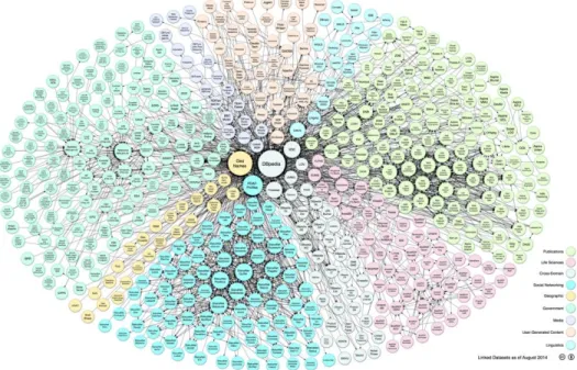
Figure 2-1 Linking Open Data cloud
(Source: by Richard Cyganiak and Anja Jentzsch http://lod-cloud.net/)
The Semantic Web takes the solution of Web further. It involves publishing in languages specifically designed for data: Resource Description Framework (RDF), The Web Ontology Language (OWL), and Extensible Markup Language (XML). HTML describes documents and the links between them. RDF, OWL, and XML, by contrast, can describe arbitrary things such as people, meetings, or airplane parts. These technologies are combined in order to provide descriptions that supplement or replace the content of Web documents [30].
2.2 Resource Description Framework
The Resource Description Framework (RDF) is a widely used model for data interchange which has been standardized into a set of W3C specifications. RDF is intended for describing web resources and the relationships between them. RDF expressions are in the form of
subject-7
predicate-object statements. These statements are also known as (s; p; o) tuples or more shortly, triples. A collection of triples can be modeled as a directed, labeled graph. If each triple has a graph name (or context), it is called a quad. Below is an example of a triple from the BTC 2012 dataset [31]:
<http://data.linkedmdb.org/resource/producer/10138>
<http://data.linkedmdb.org/resource/movie/producer_name> “Mani Ratnam”.
The above triple can be extended to a quad by adding the context: <http://data.linkedmdb.org/resource/producer/10138>
<http://data.linkedmdb.org/resource/movie/producer_name>“ManiRatnam” <http://data.linkedmdb.org/data/producer/10138>.
Resources are uniquely identified using URIs (Uniform Resource Identifiers). Resources are described in terms of their properties and values. A group of RDF statements can be visualized as a directed, labeled graph. The source node is the subject, the sink node is the object, and the predicate/property is the edge. Quads extend the idea of triples by adding a fourth entity called a context. The context names the graph to which the triple belongs. Triples with the same context belong to the same graph. RDF data may be serialized in a number of different formats, but the most common ones are RDF/XML, Notation-3 (N3), Turtle (TTL), NTriples (NT), NQuads (NQ).
2.3 Property Graph
The term property graph has come to denote an attributed, multi-relational graph. That is a graph where the edges are labeled and both vertices and edges can have any number of key/value properties associated with them [32]. The property graph data model of GraphX combines the graph structure with vertex and edge properties. Formally, a property graph is a directed multigraph and can be defined as PG(P) = (V, E, P) where V is a set of vertices and E = {(i, j) | i,
8
j
∈
V} a set of directed edges from i (source) to j (target). Every vertex i∈
V is represented by a unique identifier. PV(i) denotes the properties of vertex i∈
V and PE(i, j) the properties of edge (i,j)
∈
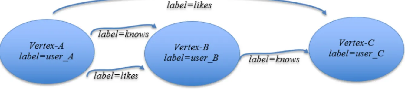
E. P = (PV , PE) is the collection of all properties. The separation of structure and properties is an important design aspect of Apache GraphX as many applications preserve the structure of the graph while changing its properties. In RDF [33] the basic notion of data modeling is a so-called triple t = (s, p, o) where s is called subject, p predicate and o object, respectively. It can be interpreted as an edge from s to o labeled with p, → . An RDF dataset is a set of triples and hence forms a directed labeled graph/ directed acyclic graph (DAG).For example, the corresponding property graph representation of an RDF graph
G1 = {(user_A, knows, user_B), (user_A, likes, user_B), (user_A, likes, user_C), (user_B,
knows, user_C)} is illustrated in Figure 1. For brevity, we use a simplified notation of RDF without information resource identified (IRIs).
9
Figure 2-2 Property graph representation of RDF graph G1
RDF triples belong to the set: ∪ × ∪ ∪ where U are URIs, L are literals and B are blank nodes and all three are disjoint sets. An RDF term is ∪ ∪ and an RDF element is any subject, predicate or object [34].
Blank nodes are used to identify unknown constants. Blank nodes are useful for making assertions where something is an object of one statement and a subject of another. For example, the director of X is Godard and the year of X is 1970. A query can be issued for what Godard directed in 1970 and X will be the result.
2.4 SPARQL
SPARQL is the standard query language for RDF data, recommended by W3C [35]. The fundamental operation in RDF query processing is Basic Graph Pattern Matching [36]. A Basic Graph Pattern (BGP) in a query combines a set of triple patterns. For example, the SPARQL query Q in Figure 2-2 retrieves a single result (or pattern mapping) for the RDF graph G1 in Figure 2-1: {(?A → user_A, ?B → user_B, ?C → user_C)}
10 SELECT * WHERE { ?A knows ?B . ?A likes ?B . ?B knows ?C }
Figure 2-3 SPARQL query Q
A Basic Graph Pattern (BGP) in a query combines a set of triple patterns. BGP queries are a conjunctive fragment which expresses the core Select-Project-Join paradigm in database queries [34]. The SPARQL triple patterns (s, p, o) are from the set:
∪ ∪ × ∪ × ∪ ∪ ∪
where U are URIs, L are literals, B are blank nodes, and V are variables [34]. The variables in the BGP are bound to RDF terms in the data during query processing via subgraph matching. Join operations are denoted by using common variables in different triple patterns. SPARQL's GRAPH keyword [36] can be used to perform BGP matching within a specific graph (by naming it) or in any graph (by using a variable for the graph name).
More formally, the basic notion in SPARQL is a so-called triple pattern tp = (s0 , p0 , o0 ) with s0 = {s’,s},p0= {p’, p} and o0 = {o’,o}, i.e. a triple where every part is either an RDF term (called bound) or a variable (indicated by ? and called unbound). A set of triple patterns forms a basic graph pattern (BGP). Consequently, the query in Figure 2-2 contains a single BGP
bgpQ = {tp1, tp2, tp3} with tp1 = (?A, knows, ?B), tp2 = (?A, likes, ?B) and tp3 = (?B,
11 2.5 Apache Spark
Apache Spark is an open source cluster computing framework. Originally developed at the University of California, Berkeley's AMPLab, later it became part of the Apache Software Foundation that has maintained it since. Spark provides an interface for programming entire clusters with implicit data parallelism and fault-tolerance [37]. ,Spark [38] is a general-purpose in-memory cluster computing system that can run on Hadoop cluster. The central data structure is a so called Resilient Distributed Dataset (RDD) [39] which is a fault-tolerant collection of elements that can be operated on in parallel. Spark attempts to keep an RDD in memory and partitions it across all machines in the cluster. Conceptually, Spark adopts a data-parallel computation model that builds upon a record-centric view of data, similar to MapReduce of Hadoop ecosystem. Spark also provides a pair RDD, which is a distributed collection of (key, value) pairs. Operations can be performed on the RDDs/pair RDDs such that the items are processed in parallel. A user can control the partitioning of the RDDs/pair RDDs in the cluster using Spark’s APIs.
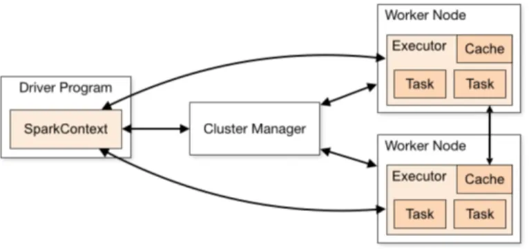
The execution model of Spark is shown in Figure 2-4. Spark uses a master/slave architecture. It has one central coordinator (Driver) that communicates with many distributed workers (executors). The driver and each of the executors run in their own Java processes.
2.5.1 Driver
The driver is the process where the main method runs. First, it converts the user program into tasks and after that, it schedules the tasks on the executors.
2.5.2 Executors
Executors are worker nodes' processes in charge of running individual tasks in a given Spark job. They are launched at the beginning of a Spark application and typically run for the
12
entire lifetime of an application. Once they have run the task they send the results to the driver. They also provide in-memory storage for RDDs that are cached by user programs through Block Manager.
2.5.3 Application Execution Flow
The process running the main() of the application is called the driver program. The executors are processes launched for the application on the worker nodes. These executors run the tasks of the application and manage the application data on disk and memory. Each application has its own set of executors. The driver program can operate with different kinds of cluster managers. In stepwise it follows like below-
1) With this in mind, when you submit an application to the cluster with spark-submit this is what happens internally:
2) A standalone application starts and instantiates a SparkContext instance (and it is only then when you can call the application a driver).
3) The driver program asks for resources to the cluster manager to launch executors. 4) The cluster manager launches executors.
5) The driver process runs through the user application. Depending on the actions and transformations over RDDs task are sent to executors.
6) Executors run the tasks and save the results.
7) If any worker crashes, its tasks will be sent to different executors to be processed again. In the book "Learning Spark: Lightning-Fast Big Data Analysis" they talk about Spark and Fault Tolerance.
13
8) With SparkContext.stop() from the driver or if the main method exits/crashes all the executors will be terminated and the cluster resources will be released by the cluster manager.
Figure 2-4 : Spark's execution model in a cluster
(Source: http://spark.apache.org/docs/latest/cluster-overview.html)
A job is modeled as a directed acyclic graph (DAG) of tasks where each task runs on a horizontal partition of the data. Apache Spark requires a cluster manager and a distributed storage system. For cluster management, Spark supports standalone (native Spark cluster), Hadoop YARN, or Apache Mesos. For distributed storage, Spark can interface with a wide variety, including Hadoop Distributed File System (HDFS), MapR File System (MapR-FS), Cassandra, OpenStack Swift, Amazon S3, or a custom solution can be implemented. Spark also supports a pseudo-distributed local mode, usually used only for development or testing purposes, where distributed storage is not required and the local file system can be used instead; in such a scenario, Spark runs on a single machine with one executor per CPU core [40].
14 2.6 GraphX
Spark also comes with a rich stack of high-level tools, including an API for graphs and graph-parallel computation called GraphX [41]. It adds an abstraction to the API of Spark to ease the usage of graph data and provides a set of typical graph operators. It is meant to bridge the gap between data-parallel and graph-parallel computation in a single system such that data can be seamlessly viewed both as a graph and as collections of items without data movement or duplication. Graph-parallel abstraction builds upon a vertex-centric view of graphs where parallelism is achieved by graph partitioning and computation is expressed in the form of user-defined vertex programs that are instantiated concurrently for each vertex and can interact with adjacent vertex programs. Internally, a graph is represented by two separate collections for edges (EdgeRDD) and vertices (VertexRDD). The graph operators of GraphX are likewise expressed as a combination of data-parallel operations on these collections in Spark with additional graph-specific optimizations inspired from specialized graph processing systems. For example, as many graph computations need to join the edge and vertex collection, GraphX maintains a routing table co-partitioned with the vertex collection such that each vertex is sent only to the edge partitions that contain adjacent edges. This way, GraphX achieves performance parity with specialized graph processing systems (e.g. Giraph and GraphLab) [26].
15 2.7 Related Work and Motivation
2.7.1 Related Work
As RDF is becoming popular from last decade, many approaches have been developed for indexing and querying RDF data. Overall, there are two storage and query processing categories of RDF solutions: centralized and distributed. Our approach is in distributed manner.
In parallel RDF query processing, available projects are Trinity.RDF [42], H2RDF+ [43], TriAD [44], DREAM [45], S2X [27] and S2RDF [26].
2.7.2 Motivation
Apache Spark’s framework GraphX has the capability to perform graph analytics on any graph. We motivate our work with basic in memory processing capability of Spark. Our work is the approaches outlined in the related work above were designed for processing of RDF triples, in distributed manner. This work also includes the capability of Jena indexing at local to the cluster and that was also the part of the motivations.
16
CHAPTER-3
PROPOSED APPROACH
3.1 Proposed Architecture
Linked Data [46], is the most popular use case for RDF on the Web where it can be used in developing an RDF knowledge base. The knowledge base is expected to contain a large number of RDF graphs where each graph may or may not be related to another graph. An RDF dataset having a large number of graphs can be processed and solved by parallel SPARQL query processing using Apache Spark and GraphX. Our design is capable of storing, indexing, and query processing massive RDF knowledge bases with a trillion triples or more, in distributed fashion.
17
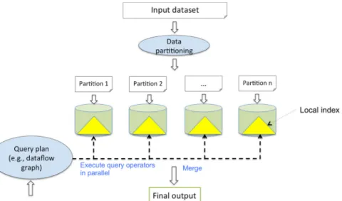
Parallel query processing has been widely studied in the context of relational databases [47]. As shown in Figure 3-1, this is the typical strategy [47], that has been described in following way-
The input dataset is RDF dataset of trillions of triples. This dataset is partitioned and distributed across a set of cluster nodes using round-robin, range partitioning, or hash partitioning schemes. Each partition is organized to execute query operators locally in an efficient manner (e.g., using indexes). An input query is mapped into a dataflow graph. This graph contains relational query operators and new operators (e.g., merge, split) that can be parallelized. The partial results can be split and merged in multiple stages to obtain the final output.
While a similar approach can be pursued for parallel RDF query processing, we make a few assumptions to simplify our design. First, we assume that the RDF dataset contains a collection of RDF graphs and has connected components. This implies that the data partitioning step can be accomplished by simply identifying connected components. In case, the dataset has a single connected graph, then we must employ graph partitioning techniques [48]. Second, for future implementations, we aim to speed up the matching of Basic Graph Patterns (BGPs) in a SPARQL query. A BGP is a connected graph. Therefore, each BGP can be executed in parallel on the partitions independently or in an embarrassingly parallel manner. If graph partitioning is used, then we need to replicate the cut edges of the RDF data graph and use a technique like n-hop replication [48] to execute BGPs independently on the partitions. A simple merging of partial results is sufficient to produce the final output. It is possible to construct complex SPARQL queries with disconnected graph patterns. In such a case, post-processing would be
18
required once the individual (connected) graph patterns are matched. Essentially, the core task is to parallelize the matching of connected graph patterns. Finally, as we are interested in handling an RDF dataset with a trillion triples or more—essentially 100’s of GBs in size—it is fair to assume that the dataset will be stored using a popular file system like the Hadoop Distributed File System (HDFS).
Given the aforementioned assumptions, we propose our approach for parallel SPARQL query processing. In this approach, we will leverage Resilient Distributed Datasets (RDDs) and MapReduce in Spark and the graph processing capability of GraphX. The key idea is to partition the RDF dataset, build indexes on the partitions after grouping them according to connected components, and execute a query in parallel on the collection of indexes. Our design aims to leverage in-memory processing of the indexes for fast query processing.
3.2 Proposed Approach
This approach is how to parallelize single SPARQL query execution, using indexing with the help of Apache Jena. In this approach, parallelism is being taken care by Apache Spark and GraphX.
3.2.1 Overall Steps
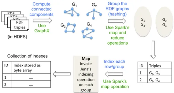
Before delving into the algorithms, we provide an overview of the index construction process and the query processing strategy for parallelizing the execution of an SPARQL query. In Figure 3-2, we illustrate the index construction process on an RDF dataset stored in HDFS. We start by partitioning the dataset by extracting the connected components in it. The connected
19
components are organized into groups. On each group, which is essentially a collection of RDF triples, we build an index using Jena. The collection of specialized indexes of Jena is stored as an RDD. Each row of the RDD holds one Jena index as a byte array. In my research, indexes reside on disk rather than in byte arrays but could be in byte array.
Figure 3-2 Overview of steps during index construction
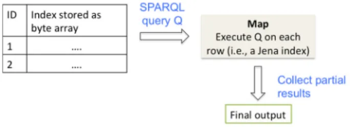
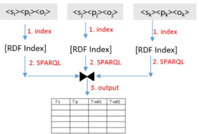
Next, we illustrate in Figure 3-3 how we process an SPARQL query in parallel. We execute the query on the collection of Jena indexes in an embarrassingly parallel manner. The partial results are simply collected to produce the final output.
20
Figure 3-3 Overview of steps during query processing
Since Spark can load an RDD into main memory for processing, we anticipate significant performance gains during query processing by operating on the Jena indexes in main memory.
3.2.2 Data Partitioning
At first glance, data partitioning appears to be straightforward. However, it poses an interesting challenge. Using Apache GraphX’s API of connected components [49], we could calculate connected components and group them as per their connected component’s unique ID. The connected components algorithm labels each connected component of the graph with the ID of its lowest-numbered vertex. With GraphX’s API, we load the RDF triples and assigns vertex IDs to the entities using a single-threaded application before invoking Spark’s APIs for creating the property graph. As our input dataset is distributed in a cluster, it is impractical to collect all the RDF triples on one cluster node and assign unique vertex IDs.
Therefore, we propose a parallel method for building the property graph from an HDFS file containing RDF triples.
21 3.2.3 Jena Indexing
Apache Jena, is an open source Semantic Web’s framework, provides an API to extract data from and write to RDF graphs. The graphs are represented as an abstract "model". A model can be sourced with data from files, databases, URLs or a combination of these. A Model can also be queried through SPARQL. In our approach we are using Apache Jena as indexing each group, further SPARQL query is being thrown on each set of indexes to retrieve results.
22
CHAPTER-4
IMPLEMENTATION OF THE SYSTEM
Our Approach’s core model of computation is relying on Apache GraphX, which is a graph processing framework built on the top of Apache Spark. Implementation of the system is divided into distinct modules: the property graph creation, creation of connected components, grouping the connected components, storing grouped components locally to each data node and apply indexing on each group.
4.1 Creation of Property Graph
We implemented a parallel method for building the property graph from an HDFS file containing RDF triples. The steps are outlined in Algorithm 1.
We first identify all the unique entities in the dataset, i.e., subjects and objects, and store them in an RDD. Then we assign a unique ID to each entity in a distributed manner. For this, we partition the range of 64-bit integers (in the driver program) and use the broadcast feature of Spark to inform all the executors of the partitioned ranges. The RDD containing unique entities is operated on, where the entities in each partition of the RDD are assigned unique IDs sequentially using a particular range. We use an interesting sequence of maps, mapPartitions and joins operations to output the vertex set and edge set of the property graph. All of the Spark’s Code, we use Scala APIs [50] for graph computations.
23
ALGORITHM 1. Converting an HDFS file containing RDF triples into a property graph
Input: An HDFS file “input.nt”containing RDF data in the N-Triples format (i.e., “subject predicate object .”on each line)
Output: A property graph representation of the RDF data
// Driver logic to make property graph
1. var file = open “input.nt”
2. var triples: PairRDD = file.mapPartition(func: getTriples) 3. var sub: RDD = file.mapPartition(func: getSubjects) 4. var obj: RDD = file.mapPartition(func: getObjects)
// Union the two RDDs and keep only the distinct entities
5. var distinctSubObj = sub.union(obj).distinct()
// Assign numeric ranges to each executor for giving a unique ID to each entity (subject or object)
6. var intRanges[(BigInt, BigInt)]: denotes an array of (BigInt, BigInt)
7. Split 64-bit integer range [0, 264) into N partitions, where N = distinctSubObj.partitions.size 8. Assign these ranges to intRanges[BigInt, BIgInt]
// All the executors will have a copy of this array
9. broadcast intRanges[BigInt, BigInt]
// Assign unique ID to each entity
10. varentityIDMapping: PairRDD = distinctSubObj.mapPartitionWithIndex(func: assignIDs)
// Generate the VertexArray for the property graph
// Contains (ID, value) pairs, where ID is a 64-bit identifier and value is the subject or object of an RDF triple
11. varvertexArray: VertexRDD = entityIDMapping.map(func: genVertexArrayTuples)
// Use join and map operations to construct the EdgeArray
24
// Contains (subID, objID, pred), where subID is an ID of the subject, objID is the ID of the object, and
// pred is the predicate of the triple
13. var edgeArray: PairRDD = temp.join(entityIDMapping).mapPartition(func: genEdgeArrayTuples)
// Property graph is ready for the next stage
14. var propGraph = Graph(vertexArray, edgeArray)
15. return propGraph
// All the map functions are listed below
func: getSubjects(myBlock)
foreach(s, p, o) triple in myBlock emit(s)
func: getObjects(myBlock)
foreach(s, p, o) triple in myBlock emit(o)
func: getTriples(myBlock)
foreach(s, p, o) triple in myBlock emit(s, (p, o))
func: assignIDs(myBlock, myID)
count = intRange[myID].begin foreach k in myBlock
// Output an assignment for a sub or obj emit(k, count++)
func: genVertexArrayTuples(myBlock)
foreach (s, ID) in myBlock emit (ID, s)
func: makeObjAsKey(myBlock)
foreach (s, (ID, p, o)) in myBlock emit (o, (ID, p))
func: genEdgeArrayTuples(myBlock)
foreach (o, ((IDs, p), IDo)) in myBlock emit (IDs, IDo, p)
As per Algorithm of building property graph, we pass RDF data from HDFS into Spark’s driver, followed by mapPartitions() we extract subjects, predicates, and objects separately. All unique ID’s has been given to distinct subject or objects. We use a sequence of transformations of Spark’s API [51] to get Vertex RDD and Edge RDD for the graph.
25
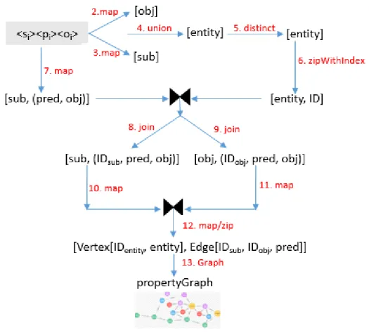
In Figure 4-1, we illustrate the transformation of RDF triples (stored in an HDFS file) into a property graph (of GraphX) according to Algorithm 1. In this figure, we show the flow of data through RDDs and pair RDDs using transformations such as map, join, union, and distinct. Each transformation (denoted by a directed edge) is labeled with the line number in Algorithm 1 and the specific operation invoked during the transformation.
Figure 4-1 Dataflow diagram depicting the transformation of an RDF dataset into a property graph using the primitives of Spark
26 4.2 Creation of Connected Components
Any property graph in Spark GraphX contains vertex RDD and edge RDD. To use Spark GraphX’s inbuilt mechanism of creating connected components, we need any property graph with vertex RDD and edge RDD. By passing obtained property graph to connected component algorithm, we get connected components. The connected component algorithm [52] labels each connected component of the graph with the ID of its lowest-numbered vertex. For example, in a social network, connected components can approximate clusters of friends.
4.3 Grouping of Connected Components
Grouping of connected components is making any number of groups as per the number of the number of requirements of the use case. To make groups we use Spark’s rangePartition() method to make sure groups are uniformly created inside the cluster.
27
4.4 Distributing Grouped Connected Components into Local to the Data Node
Spark’s API mapPartion() on any RDD could call any method to distribute data into data nodes. Our system uses mapPartion() with toLocalIterator() to distribute grouped data and store into data nodes.
4.5 Indexing Grouped Connected Components
Apache Jena is used create indexing on each grouped data on local. We use Apache Jena in a distributed manner, so that on each bucket of grouped data, it is being called parallel. Created indexes are saved at local to the data nodes.
Given the property graph representation of the RDF dataset, we will construct (in parallel) a collection of Jena indexes. We first identify connected components in the property graph using the API of GraphX. Depending on how many indexes we wish to have, which would depend on the cluster setup and the size of the RDF dataset, we create groups of connected components using some similarity criteria (e.g., Jaccard index). For each group, we generate the RDF triples in the N-Triples format and store the triples as a row of an RDD. Finally, we execute Jena’s indexing operation on the RDD resulting in a pair RDD containing the collection of Jena indexes. Each Jena index is stored as a byte array in the pair RDD. The steps are listed in Algorithm 2.
ALGORITHM 2. Index Construction
Input: A property graph propGraph
Output: A (K,V) RDD where K is an ID and V is an index on a subset of the data
28 // Driver logic
// Compute the connected components
1. var cc = propGraph.computeConnectedComponents()
// Join with the original graph so that each vertex knows it’s connected component ID and then extract the
triplets
2. var triplets = propGraph.join(cc).triplets()
// Store the property graph in an RDD where each row has an ID and an RDF graph (in the N-Triples format)
3. var rdfGraphs = triplets.mapPartition(func: genRDFTriples).reduceByKey(func: concat)
// Group the RDF graphs based on some hashing scheme
4. var rdfGraphGroups = rdfGraphs.map(func: hashAnRDFGraph).reduceByKey(func: concat)
// Invoke a tool like Apache Jena to index all the triples in a group
5. var rdfIndexes = rdfGraphGroups.map(func: invokeIndexer)
6. return rdfIndexes
// All the map operations
// For generating RDF statements in N-Triples format
func: genRDFTriples(myBlock)
foreach (tuple, ccID) in myBlock
emit(ccID, String(“tuple.src.attr tuple.attr tuple.dest.attr .\n”))
func: concat(myKey, List<NTriples>)
var allTriples func(concatenate all the RDF statements in N-Triples format) emit(myKey, allTriples)
func: hashAnRDFGraph(ID, myRDFGraph)
hashID func(apply a hash function on ID and/or myRDFGraph)
// One simple hashing scheme is to return someHashFunction(ID) emit(hashID, myRDFGraph)
func: invokeIndexer(ID, myNTriples)
invoke Jena’s tdbloader on myNTriples to construct an index create a byteArray of the index
29
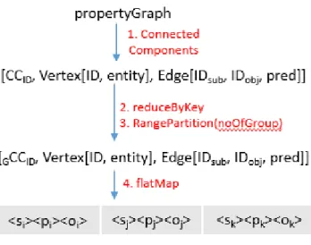
Figure 4-3 Dataflow diagram depicting the construction of RDF indexes from a property graph representation of RDF data using the primitives of Spark and GraphX
In Figure 4-3, we illustrate how the property graph is used to build a collection of Jena indexes according to Algorithm 2. Each transformation (denoted by a directed edge) is labeled with the line number in Algorithm 2 and the specific operation invoked during the transformation.
4.6 Query Execution
Given a query, we execute the query in parallel on the collection of indexes using the map operation. Each map invokes Jena’s query processing feature on an index. The partial results are simply merged/collected to produce the final output. The steps are listed in Algorithm 3.
System is capable to execute query in both ways, with the use of indexes created by Apache Jena or without indexing on grouped data.
ALGORITHM 3. Executing a single SPARQL query
Input: A SPARQL query Q and an RDD of indexes called rdfIndexes
30 // Driver logic
1. var output = rdfIndexes.map(func: runQuery, Q)
// Print the query output
2. output.collect().foreach(println)
3. return
// All the map operations
func: runQuery(Q, myIndex)
31
CHAPTER-5
PERFORMANCE EVALUATION
In this chapter, we present the performance evaluation of our purposed system, “Parallel SPARQL Query Execution Using Apache Spark”. We compared our purposed approach with existing solutions available i.e. S2X [27] on same environment, which is described in this chapter.
5.1 Experimental Setup
All experiments are done on Spark Cluster with one master and sixteen slave nodes. We have used Hadoop’s YARN as a resource manager and submitted our application jar on YARN. We use a cluster from CloudLab [53], where each machine (master/slave) is with Ubuntu 15.10 (GNU/Linux 4.2.0-27-generic aarch64), each had an 8-core CPU and 64GB RAM. We have used Apache Spark 1.6.0 version with Apache GraphX, Apache Hadoop 2.6.4, Apache Jena 3.0.1, Scala 2.11.7 on Java JDK 1.8.0_91. With our best understanding we have changed Spark’s running configuration parameter as well and same parameter’s we have used for S2X. To do experiments we have used following general parameters including Java heap of 4Gb -
MASTER="--master yarn-cluster" EXEC_NUM="--num-executors 16" DRIVER_MEM="--driver-memory 40g" EXEC_MEM="--executor-memory 50g" DRIVER_CORES="--driver-cores 6" EXEC_CORES="--executor-cores 6"
32
As we are submitting our application on YARN so accordingly we are using yarn-site.xml configuration parameters. Out of 64 Gb of RAM on each YARN we’re using around 60 Gb for YARN’s resource manager and remaining would be used by other services including Data Node, Node Manager, JVM etcetera. In yarn-site.xml our yarn.scheduler.maximum-allocation-mb (max container size) is around 60 Gb and yarn.scheduler.minimum-allocation-mb (min container size) is 2 Gb. yarn-site.xml config: <property> <name>yarn.nodemanager.resource.memory-mb</name> <value>59904</value> </property> <property> <name>yarn.scheduler.maximum-allocation-mb</name> <value>59904</value> </property> <property> <name>yarn.scheduler.minimum-allocation-mb</name> <value>2048</value> <property>
As per above parameters each time when we submit jar/job to master of YARN, 16 resource managers are requested and hence 16 executors run in cluster. Each data node would be having one executor of 6 CPU cores with 59904 mb memory.
To use memory/CPU utilization in capacity-scheduler.xml configuration we are using
org.apache.hadoop.yarn.util.resource.DominantResourceCalculator which is more useful compared to org.apache.hadoop.yarn.util.resource.DefaultResourceCalculator when we look for resources such as Memory, CPU etc.
capacity-scheduler.xml config:
33
<name>yarn.scheduler.capacity.resource-calculator</name>
<value>org.apache.hadoop.yarn.util.resource.DominantResourceCalculator</value> <description>
The ResourceCalculator implementation to be used to compare Resources in the scheduler.
The default i.e. DefaultResourceCalculator only uses Memory while DominantResourceCalculator uses dominant-resource to compare multi-dimensional resources such as Memory, CPU etc.
</description> </property>
Although in Spark 1.6.x and onwards memory management has been changed but still to make use Apache Spark’s memory management at our best level we have used following configuration and remaining setting were as default.
#GENERAL_CONFIG MASTER="--master yarn-cluster" EXEC_NUM="--num-executors 16" DRIVER_MEM="--driver-memory 40g" EXEC_MEM="--executor-memory 50g" DRIVER_CORES="--driver-cores 6" EXEC_CORES="--executor-cores 6" #EXTRA_CONFIG SPARK_CONF_SPARK_AKKA="--conf spark.akka.frameSize=1200" SPARK_CONF_SPARK_COMPRESSION="--conf spark.io.compression.codec=lzf" SPARK_CONF_SPARK_RESULTS="--conf spark.driver.maxResultSize=4g" SPARK_CON_SPARK_PARALLEL="--conf spark.default.parallelism=16" SPARK_CONF_SPARK_NETWORK_TIME="--conf spark.network.timeout=300 "
34 SPARK_CONF_SPARK_RDD_COMPRESSION="--conf spark.rdd.compress=true" SPARK_CONF_SPARK_RDD_BROADCAST="--conf spark.broadcast.compress=true" SPARK_CONFIG_RDD_SHUFFLE_SPILL="--conf spark.shuffle.spill.compress=true" SPARK_CONF_RDD_SHUFFLE_COMP="--conf spark.shuffle.compress=true" SPARK_CONF_RDD_SHUFFLE_MANAGER="--conf spark.shuffle.manager=sort" SPARK_EVENT_LOG="--conf spark.eventLog.enabled=true" SPARK_LOG="--conf spark.eventLog.dir=hdfs://128.110.152.127:9000/SparkHistory" # YARN' CONF SPARK_CONF_YARN_EX_MO="--conf spark.yarn.executor.memoryOverhead=4608" SPARK_CONF_YARN_DR_MO="--conf spark.yarn.driver.memoryOverhead=4608"
5.2 Dataset and Queries
We use real datasets for evaluating the performance and scalability of the proposed ideas. An RDF dataset generated from Data.gov [2], has been used here. The dataset contained of 52.8 million triples, which contains 1642 connected components. All datasets were cleaned before processing and, after cleaning them it was in <subject> <predicate> <object> format.
As per data set queries were formatted with two and more BGPs patterns. Full text with visualization of these star queries are in Appendix A.
5.3 Process of Execution
System consists of three modules viz. creation of connected components, grouping of connected components, indexing of each group using Jena, execution of each query on indexed data set or on dataset without indexed. All modules are single time process except the last one to execute queries.
35
5.4 Performance Evaluation and Evaluation Metrics
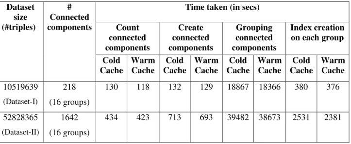
We are interested in measuring the query response time on the queries related to dataset. In this experiment setup we did evaluation on queries listed in Appendix-A. During query performance we also kept in mind regarding cold cache and warm/hot cache of the memory. We are not much interested in time spent to create connected components, grouping connected components as per connected component’s id, or even indexing the grouped data because these all are involved with only one-time execution of the module. Table 1 shows one-time execution module’s result on dataset. We execute query execution module multiple times as per required. As mentioned earlier query execution could be without indexing the grouped data or we could do Jena RDF indexing, and later submit query. Table 2 shows query result time with warn and cold caches.
Table 1 Time taken to create connected components, grouping and indexing each group
Dataset size (#triples) # Connected components
Time taken (in secs)
Count connected components Create connected components Grouping connected components Index creation on each group Cold Cache Warm Cache Cold Cache Warm Cache Cold Cache Warm Cache Cold Cache Warm Cache 10519639 (Dataset-I) 218 (16 groups) 130 118 132 129 18867 18366 380 376 52828365 (Dataset-II) 1642 (16 groups) 434 423 713 693 39482 38673 2531 2381
36
In both cases we have created 16 groups such that each data node/slave node has one group, each group may have one or more than one connected components.
Table 2 Time taken to execute queries with and without indexing
Query (Dataset-#) Execution on indexed data Execution on without indexed data Cold cache Time taken (in secs) Warm cache Time taken (in secs) Cold cache Time taken (in secs) Warm cache Time taken (in secs) Q1 Dataset-I 43 38 191 189 Dataset-II 109 104 352 348 Q2 Dataset-I 38 37 186 184 Dataset-II 138 122 314 302 Q3 Dataset-I 41 40 189 189 Dataset-II 146 135 337 331 Q4 Dataset-I 38 36 195 192 Dataset-II 152 136 331 331 Q5 Dataset-I 47 42 190 189 Dataset-II 134 132 345 341
On comparing and benchmarking with S2X [27] keeping all parameters same for both systems and using same cluster of 17 machines, we got better performance on purposed approach. Table 3 shows result and comparison with S2X.
37
Table 3 Results and comparison with S2X
Query (Dataset-#) Execution on indexed data Execution on without indexed data S2X Cold cache Time taken (in secs) Warm cache Time taken (in secs) Cold cache Time taken (in secs) Warm cache Time taken (in secs) Cold cache Time taken (in secs) Warm cache Time taken (in secs) Q1 Dataset-I 43 38 191 189 312 306 Dataset-II 109 104 352 348 621 616 Q2 Dataset-I 38 37 186 184 338 336 Dataset-II 138 122 314 302 625 619 Q3 Dataset-I 41 40 189 189 326 325 Dataset-II 146 135 337 331 643 634 Q4 Dataset-I 38 36 195 192 309 306 Dataset-II 152 136 331 331 619 608 Q5 Dataset-I 47 42 190 189 306 305 Dataset-II 134 132 345 341 622 618
Figure 5-1 shows visualization of the benchmarking on Dataset-II in cold mode and Figure 5-2 shows visualization of the benchmarking on Dataset-II in warm mode. We can easily see in bar chart, that our approach is better than S2X even without indexing the grouped data.
38
Figure 5-1 Results and comparison in cold cache
39
CHAPTER-6
CONCLUSION AND FUTURE WORK
In this article, we presented our approach to enable parallel SPARQL query processing using Apache Spark and GraphX. Our approach makes use of the MapReduce model for parallelizing the execution of a single SPARQL query. The query is executed in parallel on a collection of distributed indexes, one for each partition of the RDF dataset. In our purposed approach, we assign unique ID to each and every subject or predicate of RDF data. With the help of unique ID’s, we make property graph and create connected components using ID’s. We do grouping of the connected graphs such that each group has one or more than one connected graph. We do indexing of each groups in distributed way, indexing on each group is done using Apache Jena. At the query execution, we submit query in cluster so each time it would be executed on MapReduce pattern. While submission of the query, we can specify how we want to execute our query, using indexes of each partitioned data or without indexes, directly on portioned data.
For future work, we plan to expand this such that it also executes multiple queries in a distributed manner. Furthermore, we would like to optimize grouping of connected components algorithm so that it would be better in performance but here our main goal is to execute query and look for query performance. In addition, we would like to execute and build system using filtering technique (e.g. Bloom filter approach). Finally, we would like to extend our system so it could support RDF quadruples. Quadruples consists of a sequence of (subject, predicate, object) terms forming an RDF triple and an optional blank node label or Internationalized
40
Resource Identifier (IRI) labelling what graph in a dataset the triple belongs to (acts as context), all are separated by “.” after each statement. It would be interesting if we could compare our purposed system with recently released distributed system S2RDF [26].
41 APPENDIX A
42
All queries containing BGPs with description are given below. Corresponding figures shows the visual representation of each query. The common prefixes are listed below-
PREFIX dgv: <http://data-gov.tw.rpi.edu/vocab/p/744/>
PREFIX dgt: <http://data-gov.tw.rpi.edu/raw/793/data-793-00001.rdf#>
Q1: What are the values of all properties for “entry30” and “entry365” of Medicare cost reports.
SELECT ?p1 ?p2 ?val1 ?val2 WHERE { { dgt:entry30 ?p1 ?val1 }
UNION
{ dgt:entry144 ?p2 ?val2 } }
43
Q2: Find the values of the properties utilization code and initial report switch code for all Medicare cost reports.
SELECT * WHERE {
?mcr dgv:util_cd ?val1 . ?mcr dgv:initl_rpt_sw ?val2 }
Figure 6-2 Visualization of the query Q2
Q3: Giving two entries “entry30” and “entry365” of reports, match all Medicare cost reports such that the report has same property as “entry30” and it also has the same value for the property “last report switch code” as “entry365”. In addition, the report may have utilization code as “False”.
44 SELECT * WHERE { ?mcr ?p "N" . dgt:entry30 ?p ?o1 . ?mcr dgv:last_rpt_sw ?o2 . dgt:entry365 ?p1 ?o2 . OPTIONAL { ?mcr dgv:util_cd "F" } }
45
Q4: Find the values of all following properties- report status code, utilization code, fiscal year end date, fiscal intermediary receipt date, notice of program reimbursement date and last report switch status belonging to Medicare cost reports.
SELECT * WHERE { ?mcr dgv:rpt_stus_cd ?o1 . ?mcr dgv:util_cd ?o2 . ?mcr dgv:fy_end_dt ?date1. ?mcr dgv:fi_creat_dt ?date2 . ?mcr dgv:npr_dt ?date3 . ?mcr dgv:last_rpt_sw ?val3 }
46
Figure 6-4 Visualization of the query Q4
Q5: Find all Medicare cost reports which has automated desk review vendor code equal to “2” and initial report switch status as “NO”?
SELECT * WHERE {
?mcr dgv:adr_vndr_cd "2" . ?mcr dgv:initl_rpt_sw ?sw . FILTER (?sw = "N") }
47
48 BIBLIOGRAPHY
[1] Resource Descrip. Framework: August, 2014. http://www.w3.org/RDF. [2] Data.gov: March, 2015. http://catalog.data.gov/dataset.
[3] Data.gov.uk: March, 2015. http://data.gov.uk/data/search.
[4] NYTimes.com Linked Open Data: February, 2015. http://data.nytimes.com.
[5] MIT, EntrepreneurshipReview, August 2016, http://miter.mit.edu/articlehave-semantic-technologies-crossed-chasm-yet/.
[6] C. Bizer, T. Heath, and T. Berners-Lee. Linked Data - The story so far. Int. Journal on Semantic Web and Information Systems, 5(3):1–22, 2009.
[7] S. Auer, C. Bizer, G. Kobilarov, J. Lehmann, and Z. Ives. DBpedia: A nucleus for a web of open data. In Proc. of ISWC ’07, pages 11–15, 2007.
[8] Seman. Web Challenge: August, 2015. http://challenge.semanticweb.org/. [9] Linking Open Gov. Data: March, 2015. http://logd.tw.rpi.edu/.
[10] Slavov, Vail Georgiev, 2015, A new Approach for Fast Processing of SPARQL Queries on RDF Quadruples.
[11] FranziInc: August 2011. http://franz.com/about/press_room/trillion-triples.lhtml.
[12] Pregel: A System for Large-Scale Graph Processing- SIGMOD’10, June 6–11, 2010, Indianapolis, Indiana, USA.
49
[14] Apache GraphX: August, 2016. http://spark.apache.org/graphx/.
[15] Apache Flink, Introducing Gelly: Graph Processing with Apache Flink, August 2106, https://flink.apache.org/news/2015/08/24/introducing-flink-gelly.html.
[16] MapReduce: Simplified Data Processing on Large Clusters-Jeffrey Dean and Sanjay Ghemawat; OSDI 2004 .
[17] Apache Hadoop: August, 2016. http://hadoop.apache.org/.
[18] Apache Sparks: Lightning-fast cluster computing, August, 2016. http://spark.apache.org/. [19] Big Data Benchmark: August 2016. https://amplab.cs.berkeley.edu/benchmark/.
[20] T. Neumann and G. Weikum. The RDF-3X engine for scalable management of RDF data. The VLDB Journal, 19(1):91-113, 2010.
[21] J. Huang, D. J. Abadi, and K. Ren. Scalable SPARQL querying of large RDF graphs. Proc. of VLDB Endow., 4(11):1123-1134, 2011.
[22] P. Yuan, P. Liu, B. Wu, H. Jin, W. Zhang, and L. Liu. TripleBit: A fast and compact system for large scale RDF data. Proc. VLDB Endow., 6(7):517-528,2013.
[23] K. Zeng, J. Yang, H. Wang, B. Shao, and Z. Wang. A distributed graph engine for Web Scale RDF data. Proc. VLDB Endow., 6(4):265-276, Feb. 2013.
[24] M. A. Bornea, J. Dolby, A. Kementsietsidis, K. Srinivas, P. Dantressangle, O. Udrea, and B. Bhattacharjee. Building an efficient RDF store over a relational database. In Proc. of 2013 SIGMOD Conference, pages 121-132, 2013.
[25] Accelerating SPARQL queries by exploiting hash-based locality and adaptive partitioning:The VLDB Journal (2016) 25:355–380.
50
[26] Alexander Schatzle, Martin Przyjaciel-Zablocki, Simon Skilevic, Georg Lausen , S2RDF: RDF Querying with SPARQL on Spark, 2016 VLDB Endowment 2150-8097/16/06. [27] Alexander Sch¨atzle, Martin Przyjaciel-Zablocki,Thorsten Berberich, and Georg Lausen,
S2X: Graph-Parallel Querying of RDF with GraphX, VLDB 2015 Workshops (Big-O(Q) 2015) and DMAH.
[28] W3C, Semantic Web: August 2016, https://www.w3.org/2001/sw/.
[29] J. H. Tim Berners-Lee and O. Lassila. The Semantic Web. August 2016, http://www.scientificamerican.com/article/the-semantic-web/.
[30] Wikipedia: August, 2016, https://en.wikipedia.org/wiki/Semantic_Web.
[31] Billion Triples Challenge 2012 Dataset: August 2016, https://km.aifb.kit.edu/projects/btc-2012/.
[32] Defining a Property Graph: tinkerpop/gremlin, August 2016, https://github.com/tinkerpop/gremlin/wiki/Defining-a-Property-Graph.
[33] Manola, F., Miller, E., McBride, B.: RDF Primer. https://www.w3.org/TR/rdf-primer/. [34] Z. Kaoudi and I. Manolescu. RDF in the clouds: a survey. The VLDB Journal, pages 1-25,
2014..
[35] Prud’hommeaux, E., Seaborne, A.: SPARQL Query Language for RDF.http://www.w3.org/TR/rdf-sparql-query/ (2008).
[36] SPARQL 1.1: November, 2014. http://www.w3.org/TR/sparql11-query/. [37] Wikipedia: August, 2016, https://en.wikipedia.org/wiki/Apache_Spark.
51
Shenker, S., Stoica, I.: Fast and Interactive Analytics Over Hadoop Data with Spark. USENIX ;login: 34(4), 45–51 (2012).
[39] Matei Zaharia, Mosharaf Chowdhury, Tathagata Das, Ankur Dave, Justin Ma,Murphy McCauley, Michael J. Franklin, Scott Shenker, Ion Stoica: Resilient Distributed Datasets: A Fault-Tolerant Abstraction for In-Memory Cluster Computing.
[40] Apache Sparks, August, 2016: https://spark.apache.org/docs/latest/submitting-applications.html#master-urls.
[41] Apache Sparks: August 2016, http://spark.apache.org/graphx/.
[42] Kai Zeng, Jiacheng Yang, Haixun Wang, Bin Shao, Zhongyuan Wang: A Distributed Graph Engine for Web Scale RDF Data, PVLDB, August 1, 2013.
[43] Nikolaos Papailiou, Ioannis Konstantinou, Dimitrios Tsoumakos and Nectarios Koziris, H2RDF: Adaptive Query Processing on RDF Data in the Cloud, WWW 2012 Companion, April 16–20, 2012.
[44] Sairam Gurajada, Stephan Seufert, TriAD: A Distributed Shared-Nothing RDF Engine based on Asynchronous Message Passing, SIGMOD’14, June 22–27, 2014, Snowbird, UT, USA.
[45] M Hammoud, D.A, Rabbou, R. Nouri, DREAM: Distributed RDF Engine with Adaptive Query Planner and Minimal Communication, 2015 VLDB Endowment 2150-8097/15/02. [46] C. Bizer, T. Heath, and T. Berners-Lee. Linked Data - The story so far. Int. Journal on
Semantic Web and Information Systems, 5(3):1–22, 2009.
52
performance database systems. Commun. ACM 35, 6 (June 1992), 85-98..
[48] J. Huang, D. J. Abadi, K. Ren, “Scalable SPARQL querying of large RDF graphs,” in Proc. of VLDB Endow. 4 (11) (2011) 1123-1134.
[49] Apache Sparks, GraphX: August 2016, https://spark.apache.org/docs/0.9.0/graphx-programming-guide.html.
[50] Apache Spark: May 2016, https://spark.apache.org/docs/0.9.0/api/graphx/index.html# org.apache.spark.graphx.package.
[51] Apache Sparks: May 2016, http://spark.apache.org/docs/latest/api/scala/index.html# org.apache.spark.rdd.RDD.
[52] Apache Sparks, May 2016: http://spark.apache.org/docs/latest/api/scala/index.html# org.apache.spark.graphx.lib.ConnectedComponents$.
53
VITA
Hastimal Jangid received his Bachelor’s degree (B.Tech) in Computer Science and Engineering from West Bengal University of Technology, Kolkata, India in 2010. In August 2014, he came to the United States of America to start his Masters degree in Computer Science at the University of Missouri-Kansas City (UMKC), specializing in Data Science and Software Engineering. During his time at UMKC, he worked as a Student Assistant in UMKC-Residential Life. Later he also worked as Graduate Teaching Assistant in School of Computing and Engineering-UMKC to Dr. Praveen Rao for the graduate course ‘Principles of Big Data Management’. To get industrial technical, he also worked as Big Data/Java intern at Pegasys Systems and Technologies, Novi, MI in summer 2015 and Big Data Hadoop developer intern at Oalva, Inc Overland Park, KS in summer 2016. Upon completion of his requirements for the Master’s program, Mr. Jangid plans to work as a Big Data Engineer for Webbmason, Baltimore, MD.