Collaborative Optimization
1.1. Introduction
In this chapter we present and discuss most significant contributions in Multi-Disciplinary Optimization (MDO). The name multidisciplinary optimization is often taken literally. We prefer to call it collaborative design optimization. Indeed, the optimization tool is only one part which can not be separated from the total design process. The goal of collaborative optimization is not to create an automatic design process based on optimization algorithms but to allow easy interaction amongst teams from different disciplines.
Different publications related to MDO consider two types of design parameters, public parameters (shared by disciplines) and private parameters (specific to the given discipline). Unlike most contributions, we consider only public parameters in our discussion. We assume that for a given choice of public parameters, private parameters are fixed by each discipline at their optimal value.
The definition of public parameters and their range of validity are big issues in MDO. The choice of these parameters is often dictated by the ability and the ex-perience of the design engineers. The optimal design strongly depends on the set of selected public parameters. For example, for the design of an aircraft wing, the structural analysis team usually tries to increase the wing thickness and the aim of aerodynamicists is to decrease it. Parameterization is a way to help teams to find a compromise.
Chapter written by Yogesh PARTE and Didier AUROUX and Joël CLÉMENT and Mohamed MASMOUDI and Jean HERMETZ.
Shape parameters are quite difficult to handle. Engineers usually create parameters on dead meshes. Each discipline has its own mesh: inside the structure for structural analysis, on its surface for acoustic analysis, and outside it for aerodynamic analysis. For these reasons, we have to define discipline independent parameterized shapes.
Now a days standard Computer Aided Design (CAD) codes provide parameter-ization facilities taking into account different constraints such as parameter bounds, volumes, density, etc. Shape definition by CAD is an excellent way to facilitate inter-action between design teams. However, use of CAD for shape parameterization is not prevalent among engineering teams as CAD codes do not offer mesh parameteriza-tion facilities. Using CAD environment, it is only possible to build a new mesh for a given choice of design parameters. This way of generating meshes is not suitable for optimal shape design. Generally, the numerical error due to the change in topology of the mesh is too high compared to the information to be calculated, for example, the difference between very close responses. Therefore, for design involving shape optimization, mesh morphing which is a mean to achieve mesh parameterization, is recommended.
Multidisciplinary design is generally performed using a platform allowing interac-tion between analysis software and optimizainterac-tion toolboxes. The widely known soft-ware are iSIGHT, Dakota, Optimus (from LMS) and Boss Quatro [ALE 98, PAD 99, SAL 97, SAL 98]. These environments also support “black box” applications. The data and information exchange across different disciplines is permitted using XML or Python language based file parsing.
Considering these points, the discussions are organized as follows. In section 1.2, we discuss the parameter definition problem. Most classical MDO approaches are presented in section 1.3. Application of these MDO methods are illustrated in section 1.4. Application of game theory is a recent contribution of J. Périaux et al. to MDO. It will be presented in section 1.5. In section 1.6 we give a brief survey of very recent developments and alternative approaches for MDO.
1.2. Definition of parameters 1.2.1. Public parameters
In a multidisciplinary context, public parameters are design parameters shared by more than one discipline. The definition or choice of public parameters is itself a design step, and the final result strongly depends on it. The choice of the public parameters determine the interactions between different disciplines. We refer to the chapter "‘Multi parameter Shape Optimization"’ in this book for detailed discussion on parameterization.
In our opinion, the definition of parameters is a major issue in the collaborative de-sign. Despite technological developments, this problem remains difficult. The choice of public parameters is to be made by discussion amongst all disciplines involved in design and analysis. Generally, first few simulations carried out on the product allow parameter definition in a relevant way.
1.2.2. Private parameters
Private parameters are design parameters for specific discipline and are not shared by other disciplines. For example, if we consider an aircraft wing, number of ribs, their positions and their sizes may only interest the engineer in charge of structural analysis. One calls them private parameters. For a given choice of public parameters, the structure engineering department should carry out computations with an optimal configuration of private parameters.
1.2.3. Definition of public parameters
If one considers the case of shape optimization, number of parameters are infinite. In practice, one can work with a large number of parameters; for example all the nodes of the mesh can be design parameters. In this case, it is possible to find the optimal solution (of the optimization problem), but not the optimal design. The design criteria like aesthetic and manufacturability are difficult to describe and they are not taken into account by the optimization problem. By reducing number of design parameters we reduce the probability of unacceptable solutions.
However, an optimization process involving a large number of parameters can have at least two applications:
– The optimization process may compute an unexpected form and one might re-alize afterward that the computed form is far from being uninteresting, despite some unsatisfied criteria.
– In the development step, computation of the sensitivity with respect to all degrees of freedom of the problem (using adjoint methods) makes it possible to find the most sensitive regions and to create more appropriate parameters.
It is clear that in a multidisciplinary context, one can only work with a limited number of parameters.
1.2.3.1. Engineering knowledge
The knowledge base of engineers in terms of the experience they have gained in design and analysis process plays vital role, especially in the selecting shape param-eters and their bounds. For example, in aerodynamics, the allowable range for the
leading edge sweep angle of the wing and the wing curvature for the operational char-acteristics of the aircraft are decided by the engineer based on the experience gained from wind tunnel testings and operational characteristics of the existing aircrafts.
1.2.3.2. Adjoint methods
Adjoint method is an excellent way to define parameters. Using adjoint methods, different criteria of different disciplines can be combined in only one criterion in order to have a common gradient. The distribution of the gradient on the surface of the initial design indicates more sensitive parts of the shape. One can also compute a gradient for each criterion. Each gradient, defined on the surface, can be considered as a basic perturbation function. For the definition of adjoint, we refer to [CEA 86, JAM 90, MOH 01]. Automatic differentiation methods could be used for adjoint code generation [GRI 89, GRI 90, GRI 00, MOH 01, MOR 85, OST 71, ROS 92, SPE 80, STR 90, WEN 64].
These two approaches (adjoint methods and engineering knowledge) for the defi-nition of the parameters are complementary. In [TAN 02] the authors determine most significant design parameters by considering an hierarchical approach. This approach is also discussed in the chapter "‘Multiparameter Shape Optimization"’ of this book. We refer readers to this chapter for further details. The method based on control vol-umes is presented in the next section.
1.2.4. Creation of parameters
In the 90’s, commercial CAD software introduced utilities for shape parameteri-zation under constraints. These constraints can directly appear as mathematical equa-tions connecting one set of parameters to others (for example, constrained surface or volume). They can also be of geometrical nature: orthogonality, parallelism, etc.
These new tools are still not used, in-spite of incentive policy of many companies for the use of CAD parameterization facilities. The reasons being
– They are difficult to implement: It is not so easy to implement simultaneously an infinite number of shapes whereas it is already difficult to draw a fixed geometry.
– The technical communications often rely on CAD within a company. However, there is no standard format allowing parameterized geometry transfer between differ-ent software.
Other concerns appear in the particular context of collaborative design. The rele-vant parameters are not known a priori and CAD parameters may not be suitable.
1.2.4.1. Control volumes
In this section we propose an idea that could fulfill the needs of engineers. In what follows, we consider dead or fixed meshes. The method is based on the volume transformations. The central theme is to associate a parameterized volume to the mesh. The mesh nodes undergo the same perturbations as the points of the control volume.
The bivariate Non Uniform Rational B-Splines (NURBS) are a standard way for surface representation. One can imagine NURBS depending on three variables(u, v, w) for the definition of volumes. The perturbation of the control points of the NURBS leads to a natural mesh perturbation. One can use hexahedral finite elements as NURBS of degree 1 or 2. These elements are generally implemented in the com-putational part of most CAD software.
Major advantage of this method is to create a regular mesh perturbation inside each volume.
1.2.4.1.1. Mesh perturbation
The use of NURBS or finite elements both require an explicit function, which at each point (u, v, w)of the reference cube (0 ≤ u ≤ 1,0 ≤ v ≤ 1,0 ≤ w ≤ 1) associates a point(x, y, z)of the control volume (see Fig. 1.1), where
x(u, v, w) y(u, v, w) z(u, v, w) = X Pi(u, v, w) xi yi zi (1.1)
and where (xi, yi, zi)are the control points of the control volume. How to build a
Figure 1.1.Reference cube (left) and initial hexahedral element with its 8 control points (right).
perturbation of the mesh? Let us denote by(x0
i, yi0, zi0)the coordinates of the control points before perturbation, and (x1
i, y1i, z1i)the coordinates of these points after the perturbation. Let(x0, y0, z0)be a mesh node before perturbation. We first compute the triplet(u0, v0, w0)such that
x0 y0 z0 = X Pi(u0, v0, w0) x0 i y0 i z0 i . (1.2)
The coordinates of this point after perturbation are obtained using equation (1.3).
x1 y1 z1 = X Pi(u0, v0, w0) x1 i y1 i z1 i (1.3)
One should solve the system of three equations (1.2) and find the three unknowns at each node of the initial mesh. This operation should be done only once for all perturbations.
1.2.4.1.2. Perturbation of the external mesh
In acoustic or electromagnetic field analysis, only the surface of the structure is meshed. For these applications, it is possible to perturb the surface nodes using the process described in the previous paragraph because by construction these nodes are inside the control volume. In aerodynamic analysis often the domain of analysis is outside the structure. In this case, the large part of the mesh is outside the control volume. We propose to use the control volume technique to compute surface mesh perturbations, and to use traditional methods of mesh propagation for the computation of the external mesh perturbations. Some of these mesh perturbation methods are now discussed.
1.2.4.2. Mesh propagation
In the case of an external mesh, from a surface perturbation, one needs to propagate the modification to the neighboring mesh.
1.2.4.2.1. Elasticity methods
The surface perturbation is considered as an imposed displacement. Inside the domain, one solves a linear elasticity problem. In general, stiffness is an increasing function of the element volume. Initial mesh is used as a support for the computation [BAT 91].
1.2.4.2.2. Integral methods
Let us denote byF(x)an image of a pointxafter perturbation. We assume that
F(x)is known for all pointsxof the surface. The displacement of an internal point is weighted by the inverse of its distance from the surface:
F(x) = Z ∂Ωr0 F(x0) kx−x0kdx 0 ! / Z ∂Ωr0 1 kx−x0kdx 0 ! . (1.4)
This integral may be computed by using the perturbed mesh.
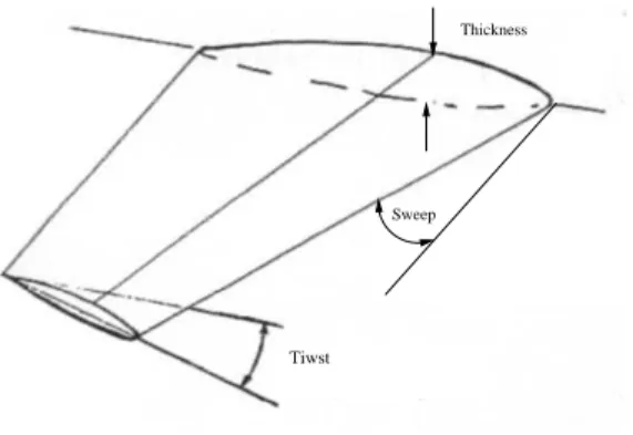
1.2.5. Application to a wing
We now consider a wing whose design variables are thickness, twist, sweep, airfoil and dihedral angle (see Fig. 1.2). We show the natural parameterization of these variables using the method of control volumes discussed earlier.
Tiwst
Sweep Thickness
Figure 1.2.Wing parameters.
A thickness modification is achieved simply by a vertical perturbation of the con-trol points of faceA(see Fig. 1.1 and 1.3). The twist parameterization is achieved by a rigid rotation of faceB (see Fig. 1.1 and 1.4). The modification in wing sweep angle consists in a rigid translation of faceB(see Fig. 1.1 and 1.5).
One can imagine a finite element of degree two if we have to modify the curvature of the airfoil or the dihedral of the wing. One can see in figure 1.6 a finite element of degree two in the plane containing the airfoil, and in figure 1.7 another finite element of degree two in the direction corresponding to the dihedral. One can see on figure
Figure 1.3.Modification of the wing thickness using a finite element of degree one in each direction.
Figure 1.4.Modification of the wing twist using a finite element of degree one in each direction.
Figure 1.5.Modification of the wing sweep using a finite element of degree one in each direction.
Figure 1.6.Modification of the wing profile using a finite element of degree two in one direction and of degree one in the two other directions.
Figure 1.7.Modification of the dihedral using a finite element of degree two in one direction and of degree one in two other directions.
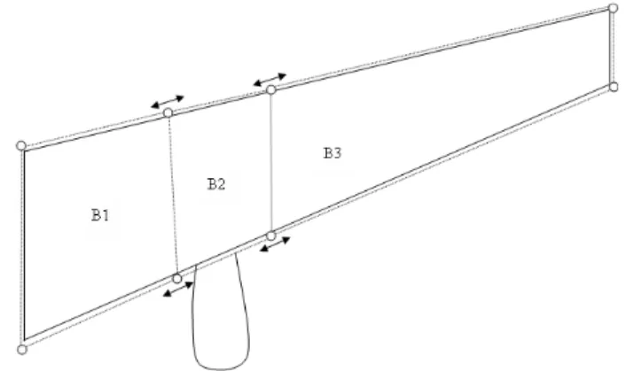
Figure 1.8.Engine displacement. The arrows correspond to the degrees of freedom of different points, other points are fixed.
1.8, the engine displacement along the wing. BlocksB1andB3follow the displace-ment induced by the control points of blockB2. If the leading edge and the tailing edge were parallel, one could only consider rigid displacements of this block. If we want to take into account the angle between these two edges, we have to force the control points ofB2to remain on the edge.
1.3. Different frameworks for collaborative optimization
In order to simplify this presentation, we limit ourselves to two disciplines and consider that private parameters are hidden under each discipline. The state equations are given in an explicit form
a1=A1(x, a2) (1.5)
a2=A2(x, a1) (1.6)
wherexrepresents public design parameters. We assume that one forgets the state, and we only take care about the output. We denote byaithe output of disciplinei. In equation 1.5,a2corresponds to the contribution of discipline2in the computation of a1and in equation 1.6,a1represents the output of discipline2in the computation of a2. Thusa1anda2also represent the coupling between two disciplines.
We want to solve the following optimization problem min
x f(x, a1(x), a2(x)) Subjected to:
g(x, a1(x), a2(x))≤0
(1.7)
In this presentation we do not consider disciplinary internal constraints; they should be implicitly taken into account by the state equations.
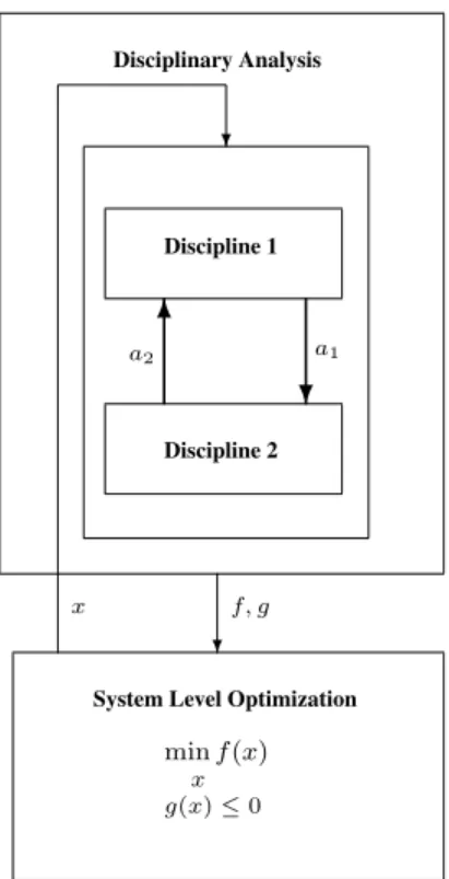
1.3.1. Multi-Disciplinary Feasible (MDF) method
In this formulation, all design variables x are provided to the coupled system of disciplinary analysis. For given design variablesx, a complete multidisciplinary analysis (MDA) is performed via a fixed-point iteration to obtain output variables
a1, a2. These outputs are then used in evaluating the objective f(x) and the
con-straintsg(x, a1, a2). The optimization problem solved at system level is:
min x f(x) Subjected to:
g(x)≤0
(1.8)
If a gradient-based method is used to solve the above problem, then a complete MDA is necessary not just at each iteration, but at every point where the derivatives are to be evaluated. Thus, attaining multidisciplinary feasibility can be prohibitively expensive in realistic application [KOD 98].
x minf(x) ? f, g g(x)≤0 Disciplinary Analysis a2 a1
System Level Optimization Discipline 1 Discipline 2 x ? ? 6
Figure 1.9.MDF framework for MDO
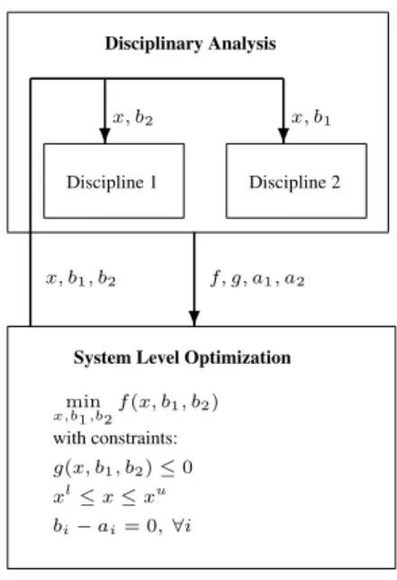
1.3.2. Individual Discipline Feasible (IDF) method
As the name suggest, the IDF formulation provides a way to avoid a complete MDA at optimization. IDF maintains individual discipline feasibility, while allowing the optimizer to drive individual disciplines to multidisciplinary feasibility and opti-mality by controlling interaction variables. The specific analysis variables that rep-resent communication, or coupling, between disciplines are treated as optimization variables. The IDF formulation is:
min x,b1,b2 f(x, b1, b2). g(x, b1, b2)≤0 b1=a1(x, b2) b2=a2(x, b1) (1.9)
? ? ? x, b1 x, b1, b2 f, g, a1, a2 bi−ai= 0,∀i g(x, b1, b2)≤0 xl≤x≤xu Disciplinary Analysis with constraints:
System Level Optimization Discipline 1 Discipline 2
min
x,b1,b2f(x, b1, b2)
x, b2
Figure 1.10.IDF framework for MDO
1.3.3. All-At-Once (AAO) method
The AAO method is also the so-called “one shot”, SAND or SAD (Simultaneous Analysis and Design) method [ALE 00b, BRA 96, GUM 01]. Simultaneously one solves state equations and the optimization problem. Contrary to the MDF method, the state equations are not supposed to be satisfied at each step of the optimization algorithm, but they are satisfied when the convergence is achieved. State equations are indeed considered as equality constraints.The optimization problem defined by this method is:
min x,b1,b2 f(x, b1, b2). g(x, b1, b2)≤0 b1=t1 b2=t2 t1 =A1(x, b2) t2 =A2(x, b1) (1.10)
This method is really efficient, but it can be difficult to obtain its convergence when some of the state equations are strongly nonlinear. Even in a mono-disciplinary con-text, the convergence is not always achieved.
1.3.4. Bi-Level Integrated System Synthesis (BLISS)
This method is described in [SOB 98]. At every stage, equations of state given by equation (1.5) and (1.6) are solved and corresponding gradients are computed using an associate method. The gradient information is used to construct an approximation of the global cost function and the constraints. The approximation of the cost function includes a term associated with Lagrange multipliers,λ, coming from the local opti-mizations. The region of confidence to ascertain reliability of these approximations is also computed. The optimization problem in terms of pointxcuris as follows:
∂xf0=∂xf(xcur, a1(xcur), a2(xcur))
∂xg0=∂xg(xcur, a1(xcur), a2(xcur))
g0=g(xcur, a1(xcur), a2(xcur)) min x (∂xf0+λ.∂xg0)(x−xcur) g0+∂xg0(x−xcur)≤0 (1−∆)xcur≤x≤(1 + ∆)xcur (1.11) -? ? ? ? MDA Update Variables xcur=xopt xopt Sub-system Optimization λ f0, g0 xcur ∂xf0, ∂xg0
System Level Optimization Global Sensitivity Equation
where,∆denotes the region of confidence.
Depending on the method used to generate approximations of the cost function and constraints, different variant of BLISS are cited in literature. The formulation BLISS-RSM [ALT 02] uses polynomial approximations as disciplinary meta-models. The formulation BLISS-2000 [AGT 00] generalizes the BLISS by using disciplinary meta-models.
1.3.5. Disciplinary Analysis Optimization (DAO) method
In DAO method [ALE 98, ALE 00b], the optimization is no more performed by disciplines. However, each discipline may change the parameters in order to obtain an admissible point. We previously assumed that the private constraints are part of the state equations. Private parameters are generally used to satisfy these constraints, but there may not exist any vectorx, representing the public variables, that is solution of the problem. This is why one usually relaxesx. Each discipline chooses its own set of public parametersziin order to satisfy its private constraints. When the convergence is achieved, allziare equal. Convergence of allziis ensured by added equality constraint of the formzi=xin the optimization problem. The optimization problem solved by DAO method is:
min x,b1,b2 fDAO(x, b1, b2). g(z0, b1, b2)≤0 b1=a1(z1, b2) b2=a2(z2, b1) z0=x z1=x z2=x (1.12)
1.3.6. Collaborative Optimization (CO) method
In the CO method [ALE 98, ALE 00b, ALE 00c, ALE 00a, BRA 96], all disci-plines contribute to the improvement of the results. We use same notations used to present DAO method. Collaborative Optimization is a bi-level optimization approach. The optimization problem is solved at the system level and the disciplinary level.
At system level we solve the following problem:
min x f(x, b1, b2) kx−z1k2+kx−z2k2+ ka1−b1k2+ka2−b2k2= 0 g(z0, b1, b2)≤0 (1.13)
The main goal of this system level optimization problem is to impose to each discipline some objectives to be reached in a least square sense. For disciplinei, output target is
biand the disciplinary solutionzishould be close tox.
The disciplinary optimization problem for discipline1is then min z1 1 2 kz1−xk2+kb1−a1(z1, b2)k2 (1.14) wherea1is the solution of the state equation (1.5).
The optimization problem for discipline2is min z2 1 2 kz2−xk2+kb2−a2(z2, b1)k2 (1.15) wherea2is the solution of the state equation (1.6).
? ? Discipline 2 kx−z1k2+kx−z2k2+ka1−b1k2+ka2−b2k2= 0 -Discipline 1 -min z1 1 2 kz1−xk2+kb1−a1(z1, b2)k2 xmin≤z 1≤xmax x, b1, b2 min z2 1 2 kz2−xk2+kb2−a2(z2, b1)k2 f, g, z1, z2, a1, a2 xmin≤z2≤xmax subjected to: Subjected to: zi=x,∀i
System Level Optimization
xmin≤x≤xmax g(z0, b1, b2)≤0 min x,b1,b2 f(x, b1, b2) subjected to:
1.3.7. Collaborative Sub-Space Optimization (CSSO) method
We will give a quick overview of the CSSO method, one can see [SHA 93] for a more detailed presentation. The design parameters are distributed between the differ-ent disciplines. Each discipline has to optimize certain parameters.
The CSSO is similar to the domain decomposition method and its application for solving state equations, except for one aspect: in domain decomposition, an unknown can easily be associated to one equation of the state. In multidisciplinary optimization, it seems hard to associate any public parameter to one particular discipline, because by definition public parameters are to be shared between different disciplines.
We will use an approximation or meta-model of discipline 2 (denoted byA˜2) in
the equation corresponding to discipline 1, and reciprocally, we use an approximation of discipline 1 (denoted byA˜1) in the equation corresponding to discipline 2.
Let us recall the initial problem
a1=A1(x, a2), (1.16)
a2=A2(x, a1), (1.17)
min
x f(x, a1(x), a2(x)).
g(x, a1(x), a2(x))≤0 (1.18)
and we setx= (x1, x2), wherexiis the vector of the variables associated to discipline
i. Then, we denote by˜aithe approximation of the output ofai. Further details about these approximations are referred to section 1.3.9.
The optimization problem for discipline 1 is:
a1=A1(x,˜a2), (1.19) ˜ a2= ˜A2(x, a1), (1.20) min x1 f(x1, x2, a1(x),˜a2(x)) (1.21) g(x, a1(x),˜a2(x)) ≤0 (1−∆2)x1cur≤x1≤(1 + ∆2)x1cur (1.22) The constraint given by equation 1.22 is introduced to set the validity domain of the approximation ofa2 around the current pointx1cur. The approximate response˜a2
In the same way, we can write the problem solved by discipline2 ˜ a1= ˜A1(x, a2), (1.23) a2=A2(x,˜a1), (1.24) min x2 f(x1, x2,a˜1(x), a2(x)). (1.25) g(x,˜a1(x), a2(x)) ≤0 (1−∆1)x2cur≤x2≤(1 + ∆1)x2cur (1.26) where constraint given by equation 1.26 is introduced to set the validity domain of the approximation ofa1 around the current pointx2cur. The approximate response˜a1
and the coefficient∆1are provided by discipline1.
Many results have been published about parameterization methods with the aim of increasing the autonomy of each discipline and enlarging the trust region [GUI 92, GUI 93, GUI 94, GUI 95, MAD 00, LAW 96, LEG 04, ROD 00, SAN 00, SER 98, SOB 00].
In most domain decomposition methods [ACH 95], there is a natural way to as-sociate unknowns to equations, and there are as many equations as unknowns. This association makes the finding the solution much easier. In collaborative design, it is not so natural to associate a sub-space to a discipline. The chapterConcurrent Opti-mizationproposes strategy for sharing different design parameters.
1.3.8. Disciplinary Interaction Variable Elimination (DIVE) method
This MDO formulation is described in [MAS 06]. It is primarily inspired by the BLISS2000 method [AGT 00]. The core idea in this formulation is to reduce the complexity of the optimization problem by a progressive elimination of different types of variables and to generalization of the trust region method.
In DIVE method each discipline is responsible for construction of its meta-model. The output of the meta-model depends only on the public parameters. For a given public parametersx, the response of each meta-model is optimal with respect to its private parameters. This constitutes disciplinary level. In this way it eliminates private variables. Along with the outputA˜ieach discipline also provides the reliability index
αi of the output. Whenαi < 0, the meta model is valid at current design point. Ifαi ≥0it is necessary to re-construct the meta-model about current design point. Meta-models can be constructed using the neural network techniques, Kriging, etc. When the meta-model is a linear or quadratic approximation, the reliability constraint
αi < 0defines what we call the trust region. On the other hand, if αi ≤ 0 in the complete design space, DIVE method is similar to other meta-model based MDO methods. For this reason DIVE method is considered as a generalization of the trust region method. 6 -? 6 ? 6 6 xoptacceptable? min a1,a2k ˜ A1(x, a2)−a1k2+kA˜2(x, a1)−a2k2 Disciplinary Level Update Meta-models System Level αi ˜ A1,A˜2 a1, a2 f, g, xopt YES NO x min x f(x) With constraints:
Elimination of coupling variables αi≤0, reliability indices of meta-models
xmin≤x≤xmax
g(x)≤0
Discipline 1 Discipline 2
Figure 1.13.Diagram for DIVE formulation
Once meta-models are constructed, coupling variablesa1anda2are eliminated by
minimizing the residue of the state equations in a least squares sense:
min a1,a2
This specific approach in DIVE to find the solution of state equations using minimiza-tion problem defer from other formulaminimiza-tions where state equaminimiza-tions are solved either using fixed point method (as in MDF, BLISS) or by adding equality constraints (as in AAO, IDF, CO). This characteristic makes DIVE a more robust method and allows use of efficient minimization techniques such as the method of Levenberg-Marquardt or the adjoint method.
After elimination of coupling variables, shared variables are treated at system level optimization. The optimization problem solved at system level is:
min x f(x)
g(x)≤0
αi≤0 (1.28)
The solution of above optimization problem is checked for following points
– If the design point obtained is on the boundary of the validity domain of any of the meta model (that isαi = 0for anyi), a new meta-model is constructed around the design point and optimization procedure is repeated.
– If state equations are not satisfied with desired accuracy, meta-models are up-dated.
In this way, DIVE formulation also provides the quality index for the obtained optimal solution. Distinguishing features of DIVE formulation are:
– In DIVE method, priority is given to accurate solution of state equations of the system.
– Peculiar construction of disciplinary meta-model provides reliability index for the disciplinary output variables and thus DIVE becomes generalization of trust region method.
1.3.9. Reduced order models and approximations
In this section we take a brief review of different meta-modeling techniques. For detailed discussion on this topic we refer to chapters,Response Surface Methodology (RSM) and Reduced Order Models (ROM),Meta-modeling using Principal Compo-nent AnalysisandModel Reduction for Coupled Problemsin this book. Meta models also known as surrogate models provide a convenient way to reduce MDO complexity. Any approximation has a local validity in an appropriate trust region, for example,
– Linearization is valid in a small region and for a large number of parameters if adjoint is considered.
1.3.9.1. First order approximation
The most simple way to build a local approximation is to differentiate (1.5) and (1.6), but its trust region is relatively small. We obtain
˜
a1=∂xA1(xcur, a2(xcur))(x−xcur)
+ ∂a2A1(xcur, a2(xcur))(a2(x)−a2(xcur)), (1.29)
and
˜
a2=∂xA2(xcur, a1(xcur))(x−xcur)
+ ∂a1A2(xcur, a1(xcur))(a1(x)−a1(xcur)). (1.30)
The adjoint method (reverse mode in automatic differentiation) could be consid-ered for large scale problems [GRI 89, GRI 90, GRI 00, MOH 01, MOR 85, OST 71, ROS 92, SPE 80, STR 90, WEN 64].
1.3.9.2. Approximation using parameterization methods
Parameterization methods are usually appropriate when the disciplines are weakly coupled. More precisely, it is assumed that one discipline is independent of the others:
a1=A1(x) (1.31)
a2=A2(x, a1). (1.32)
In this example, discipline 1 does not require any information from discipline 2. One can see this kind of approximations in the field of aeroelasticity. The output
a1usually represents the structure response to mechanical excitation (a modal analysis
is often necessary for determining the structure response). A good approximation˜a1
ofa1consists in using the same modal basis when the design parametersxvary.
To build surrogate (or reduced) models, we proceed in the following way. First we solve (1.5) and (1.6) for several vectors x. Generally, we consider Design Of Experiments (DOE) methods to select appropriate vectorsxk,k= 1,· · ·, nwheren is small.
The second step consists in building the surrogate model. There are two families of methods:
1) Approximation of objective function and constraints using surface response methods [CRI 00, PLA 99, VAP 95] like polynomial approximation, neural networks, Support Vector Machine (SVM), Radial Basis Functions (RBF), etc. ;
2) For each vector xk, we consider the corresponding solutionuk (the result of the full analysis). Then, for a given new vectorx, we look for the corresponding so-lutionuas a linear combination of vectorsuk. This problem is small and has only a n-dimensional unknown vector. From the numerical point of view, it is neces-sary to build an orthonormal basis from vectors uk. For this reason, this method is called Proper Orthogonal Decomposition (POD) [GUI 92, GUI 93, GUI 94, GUI 95, MAD 00, LAW 96, LEG 04, ROD 00, SAN 00, SER 98, SOB 00].
If we compare methods1 and2, the parameterization provided by POD takes into account the knowledge of the model. With parameterization, the evaluation of the cost function is so cheap that it is possible to consider genetic algorithms [MÄK 98, PÉR 98], and other global optimization algorithms [KEL 99b, KEL 99a, MON 99].
1.4. Application of MDO to conceptual design of super sonic business jet (SSBJ) The test case of conceptual design of super sonic business jet (SSBJ) is proposed by DASSAULT aviation as a part of the OMD-RNTL project [OMD06] to compare performance of different MDO frameworks described in previous sections. We briefly discuss main features of this test case. Detailed description of this test case is referred to [RAV 07].
Three different disciplines, namely, structures, aerodynamics and propulsion con-stitute three coupled subsystems or computational modules in the design cycle of SSBJ.
– Structures: Computes mass of different parts of an aircraft such as wing, fuse-lage, tail, engine, etc., and the take-off weight as function of geometrical parameters of an aircraft and engine mass.
– Aerodynamics: Computes the lift and drag during cruise using aircraft mass, geometrical details and engine size as input parameters. The drag estimates from aerodynamics module are used by propulsion module for engine sizing operations.
– Propulsion: Performs engine sizing and estimates the engine thrust using drag estimates generated using aerodynamic analysis. The engine mass computed by propulsion module acts as an input to the structures module.
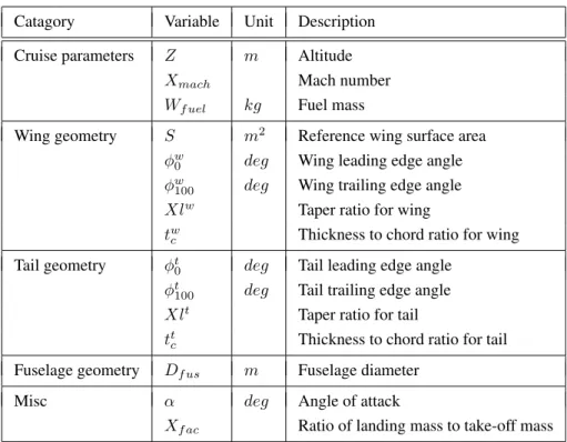
Output from these subsystems, namely the take-off weight and engine thrust consti-tute input for the performance module. The performance module computes the range, take-off distance and landing speed of an aircraft. Figure 1.14 shows the coupling be-tween different disciplines under SSBJ test case and Table 1.1 enlists different design variables, their units and symbols used for their representation.
Catagory Variable Unit Description Cruise parameters Z m Altitude
Xmach Mach number
Wf uel kg Fuel mass
Wing geometry S m2 Reference wing surface area φw
0 deg Wing leading edge angle φw
100 deg Wing trailing edge angle Xlw Taper ratio for wing
twc Thickness to chord ratio for wing Tail geometry φt
0 deg Tail leading edge angle φt100 deg Tail trailing edge angle Xlt Taper ratio for tail
tt
c Thickness to chord ratio for tail Fuselage geometry Df us m Fuselage diameter
Misc α deg Angle of attack
Xf ac Ratio of landing mass to take-off mass
Table 1.1.Different design variables in SSBJ test case
Catagory Variable Unit Description Interaction T OW kg Take-off mass
F0 N Thrust
Table 1.2.Interaction variables in SSBJ test case
The design cycle consists of iterative solution procedure to find converged val-ues of take-off weight and engine thrust under different constraints. Other design parameters such as lift, drag and engine size are functions of take-off weight and en-gine thrust. Take-off weight and enen-gine thrust thus constitute shared variables. Their converged values represents the equilibrium amongst above three disciplines. Using take-off weight and engine thrust one aircraft range is computed using Breguet equa-tion in performance module. Landing speed and take-off distance is computed using empirical relations [RAV 07]. The aim of this test case is to design SSBJ which has
Structure Landing Speed Range Drag Mass Propulsion Aerodynamics engine size Lift Engine mass Performance
Take off weight, Thrust
Take off−distance
Figure 1.14.Coupling between different disciplines under DASSAULT SSBJ test case
minimum take off weight (TOW) subjected to following constraints on aircraft range, take-off distance (Dtake-off) and landing speed (Vapproach). These constraints are:
•The aircraft range,R, should be greater than or equal to6500km
•The take-off distance,Dtake-off, should be less than or equal to1828m
•The landing speed,Vapproach, should be less than or equal to70m/s
1.4.1. Results obtained using different frameworks
The SSBJ test case is formulated as a MDO problem using DIVE, MDF, IDF and BLISS formulations discussed in section 1.3. For DIVE method, meta-models are lin-ear approximations constructed using gradient of disciplinary output variables. Table 1.3 to 1.5 shows results obtained using different MDO framework for SSBJ test case. Table 1.3 shows optimal values of design variables obtained using different MDO frameworks. Considerable differences exists in the optimal value of design variables pertaining to the geometry of the wing and tail computed by different disciplines.
– The trailing edge sweep angle,Φw100, for the wing as computed by DIVE, MDF and IDF is about5.5 degwhereas by BLISS method this values is−5.3 deg.
– The taper ratioXlwvalue for wing is less than0.05by BLISS, IDF and MDF method. Taper ratio for wing as computed by DIVE is0.11.
Variables DIVE MDF IDF BLISS min max Z (m) 14585 14985 14845 14895 8000 18500 Xmach 1.6 1.6 1.6 1.6 1.6 2 S (m2) 100 100 100 100 100 200 φw 0 (deg) 46.1 51.8 51.9 46.8 40 70 φw100 (deg) 5.5 5.6 5.4 -5.3 -10 20 Xlw 0.11 0.05 0.05 0.05 0.05 0.5 tw c 0.04 0.046 0.0463 0.04 0.04 0.08 φt 0 (deg) 56 56 57 70 40 70 φt 100 (deg) 5 5 5 0 0 10 Xlt 0.274 0.274 0.274 0.500 0.05 0.5 ttc 0.063 0.060 0.059 0.05 0.05 0.08 Df us (m) 2 2 2 2 2 2.5 Wf uel (kg) 15000 15000 15000 15000 15000 40000 α (deg) 15 15 15 15 10 15 Xf ac 0.85 0.85 0.85 0.85 0.85 0.95 T OW (kg) 33066 33207 32862 33065 1 100000 F0 (N) 62221 62704 61963 62220 1 300000 Table 1.3.Optimal design variables obtained using different MDO frameworks
– Leading edge sweep angle for the tail,Φt
0attains its maximum value whereas the
trailing edge sweep angle for the tail, Φw
100attains its minimum value using BLISS
method. Using DIVE, MDF and IDF, the leading edge sweep angle of the tail is 56 degwhereas the trailing edge sweep angle for tail is5 deg.
– Taper ratio for the tail has optimal value of0.5, which is the upper limit on the permissible values under BLISS framework and has a value of0.274 under DIVE, MDF and IDF framework.
Rest of the design parameters have more or less similar values under different MDO frameworks.
Table 1.4 shows optimal values of disciplinary outputs under different MDO frame-works. The take-off weight as computed by BLISS and DIVE is33066kgand33065
kg respectively. The take-off weight computed using IDF is32862kgand that with MDF is33207kg. It is to be observed that though take-off weight computed by IDF is minimum it is not the feasible solution as it violates constraints of landing speed.
This is due to the fact that in IDF priority is given to individual disciplinary feasibility and thus state equations are not solved accurately. Even when multi-disciplinary anal-ysis is coupled with IDF it doesn’t provide feasible solution as evident from the value of range, take-off distance and landing speed recorded under column IDF+MDA in Table 1.4. This underlines the fact that in MDO framework it is utmost important to accurately solve the state equations.
Output DIVE MDF IDF +MDAIDF BLISS min max
T OW (kg) 33066 33207 32862 33141 33065 50000
F0 (N) 62221 62704 61963 62356 62220
R (m) 6500 6501 6510 6443 6500 6500
Dtake-off (N) 1828.0 1827.3 1826.4 1842.0 1828.0 1828
Vapproach (m.s−1) 70.0 70.0 69.9 70.2 70.0 70
Table 1.4.Optimal value of output variables obtained using different MDO frameworks
Table 1.5 shows number of calls made to disciplinary analysis under different MDO frameworks. It also includes calls to disciplinary analysis to compute gradi-ent of disciplinary output variables and those required for the construction of meta-models. As evident, DIVE method requires minimum number of disciplinary
analy-Discipline DIVE MDF IDF BLISS
Structure 630 1459 1144 966
Aerodynamics 630 1459 1144 966 Propulsion 636 1490 1144 992 Performance 606 1552 1144 1044
Table 1.5.Number of calls for disciplinary analysis by different MDO frameworks
ses (about 630 for each disciplines) followed by BLISS (about 1000) and IDF. MDF formulation requires maximum number of disciplinary analyses, about 1450 for each discipline. These results also show the advantage of using meta-models at disciplinary level, as in DIVE method, rather than using system level meta models as utilized in
BLISS method. One must realize that for this test case there are only two shared or coupling variables and construction of disciplinary meta-models is easy. The final configuration obtained using different MDO methods is more or less similar. There-fore, performance index of different MDO methods is judged on the basis of compu-tational cost measured in terms of number of calls to disciplinary analysis. With this performance index DIVE method outperforms other method. However, in more com-plicated cases, construction of disciplinary meta-model itself can be computationally expensive step. None-the-less it can be concluded that in meta-model based MDO, DIVE method outperforms other methods.
1.5. Game theory
Game theory has been used for multi-criteria optimization [RAM 02]. Then, it has been enhanced by J. Périaux et al. [MÄK 98, PÉR 98, WAN 92] as an excellent way to deal with multidisciplinary optimization. Game theory seems to be more suitable for multidisciplinary design than most of classical methods. In particular, criteria like the maximum of the Von Mises stress, the drag and the lift, the maximum displacement, and the fuel consumption are of totally different nature. The main advantage of game theory is to work in a multi-criteria context, and each discipline is in charge of its own criterion.
The natural way to adapt game theory to multidisciplinary optimization is to con-sider each discipline as a player. We concon-sider two real cost functions defined onA×B:
fA: A×B → R (x, y) 7→ fA(x, y) (1.33) and fB: A×B → R (x, y) 7→ fB(x, y) (1.34) whereAandBare two parts ofRnandRmrespectively. PlayerAminimizes the cost functionfA with respect tox, while playerB minimizes the cost functionfB with respect toy.
1.5.1. The Pareto equilibrium 1.5.1.1. Definition
The point(x∗, y∗)is Pareto optimal (or a Pareto equilibrium point) if there does not exist any(x, y)∈A×Bsuch that
fA(x, y)≤fA(x∗, y∗)
or
fA(x, y)< fA(x∗, y∗)
fB(x, y)≤fB(x∗, y∗).
This is equivalent to say that there is no way to improvefAwithout a loss of perfor-mance offBand vice versa.
The set of all Pareto equilibrium points is called the Pareto front.
When the Pareto front is a convex set, one can find all its points while minimizing
fλ=λfA+ (1−λ)fBfor all0< λ <1. For allλ, there exists a Pareto equilibrium point.
The teams in charge of disciplines may use the set of the Pareto front to find a compromise.
1.5.1.2. Example
Let us consider a very simple example
fA= (x−1)2+ (x−y)2
fB= (y−3)2+ (x−y)2.
(1.35)
One can find the Pareto equilibrium points by considering a convex combination of two criteria
fλ=λfA+ (1−λ)fB, (1.36) and minimizingfλfor all0< λ <1. In this case, we have
fλ=λ(x−1)2+ (1−λ)(y−3)2+ (x−y)2 (1.37) and then ∂xfλ= 2 [λ(x−1) + (x−y)] = 0 ∂yfλ= 2 [(1−λ)(y−3)−(x−y)] = 0. (1.38) We finally obtain (1 +λ)x−y=λ −x+ (2−λ)y= 3(1−λ). (1.39)
1.5.2. The Nash equilibrium 1.5.2.1. Definition
The point(x∗, y∗)is a Nash equilibrium point if
( f A(x∗, y∗) = inf x fA(x, y ∗) fB(x∗, y∗) = inf y fB(x ∗, y). (1.40)
It is straightforward to see that this equilibrium point must satisfy the optimality system ∇xfA(x∗, y∗) = 0 ∇yfB(x∗, y∗) = 0 (1.41) 1.5.2.2. Example
We consider again example (1.35)
fA= (x−1)2+ (x−y)2
fB= (y−3)2+ (x−y)2,
(1.42) and the corresponding Nash equilibrium is given by
∂xfA= 0 ∂yfB = 0 ⇐⇒ y= 2x−1 x= 2y−3 ⇐⇒ x= 5 3 y=7 3 (1.43)
One may remark that the solution of (1.43) is exactly the same as in (1.39) with
λ= 1in the first equation andλ= 0in the second one.
The Nash equilibrium is an interesting way to avoid arbitrary weighting of cost functions. However, the compromise, between disciplines, is hidden by parameters definition. For example, the choice of the parameters subsets corresponding to disci-pline 1 and discidisci-pline 2 is a hidden compromise.
1.5.3. The Stackelberg equilibrium 1.5.3.1. Definition
We now assume that one of the two players is the leader of the game, for example playerA. The multidisciplinary problem is formulated as follows:
min
x fA(x, yx) whereyx= arg min
y fB(x, y).
(1.44)
This is an elimination method for unknown variables. Then, we only have to minimize
j(x) :=fA(x, yx). (1.45) If we assume that fA is an aerodynamics cost function, for example the drag, and thatfB is the weight, thenyrepresents the private parameters of the structural mechanics (number of spars, position, thickness, etc.). Each evaluation offBrequires the resolution of a structural mechanics optimization problem.
1.5.3.2. Example
We still consider the previous example
fA= (x−1)2+ (x−y)2
fB= (y−3)2+ (x−y)2.
(1.46)
The Stackelberg equilibrium is exactly the Nash equilibrium:
yx= (x+ 3) 2 , j(x) = (x−1)2+ x−3 2 2 .
The minimization ofj(x)gives
x=5
3 and yx= 7 3 .
1.5.4. Application of the game theory to the multidisciplinary design We simply have to consider equations (1.5), (1.6) and cost function (1.7)
a1=A1(x, a2) (1.47)
a2=A2(x, a1) (1.48)
min
x f(x, a1(x), a2(x)) (1.49)
g(x, a1(x), a2(x))≤0
where the weighted criterionf(x, a1(x), a2(x))is replaced byf1(x, a1(x), a2(x))for
discipline 1 and byf2(x, a1(x), a2(x))for discipline 2. For example, if discipline 1
is structural mechanics,f1may represent the weight of the structure. If discipline 2 is
aerodynamics, thenf2may be the lift (with a constraint on the drag).
Then, we consider the decomposition introduced in the frame of the CSSO method (see section 1.3.7). But, here the system level cost function is replaced by disciplinary
cost functions. Discipline 1 solves the following problem a1=A1(x,˜a2), (1.50) ˜ a2= ˜A2(x, a1), (1.51) min x1 f1(x1, x2, a1(x),˜a2(x)) (1.52) g(x, a1(x),˜a2(x))≤0 (1−∆2)x1cur≤x1≤(1 + ∆2)x1cur, (1.53) and discipline 2 solves the following problem
˜ a1= ˜A1(x, a2), (1.54) a2=A2(x,˜a1), (1.55) min x2 f2(x1, x2,a˜1(x), a2(x)) (1.56) g(x,a˜1(x), a2(x))≤0 (1−∆1)x2cur≤x2≤(1 + ∆1)x2cur. (1.57) One can add constraints directly in the cost function in order to be exactly in the context of game theory.
Game theory is little used in the context of multidisciplinary optimization. How-ever, at various levels, it can offer interesting answers:
– The Pareto equilibrium provides a complete range of relevant solutions. Among these solutions, one can choose the best design that satisfies subjective criteria.
– The Nash equilibrium makes it possible to avoid compromises, even if a hidden compromise lies in the choice of the subspaces of discipline 1 and discipline 2.
– The Stackelberg equilibrium is particularly well adapted to optimization with respect to private variables.
1.6. Other approaches in collaborative design
In section 1.3 we discussed different MDO frameworks in which a complex sys-tem is decomposed into subsyssys-tems based on the aspect of the involved analysis (such
as discipline specific analysis and expertise). These frameworks are motivated primar-ily by aerospace industry in which the design task is based on disciplinary analysis, for example structure, fluid dynamics, control etc. All subsystems are considered at equal level and in principle there is no restriction on communications between subsys-tems. However, in certain industries like those in automotive sector, design cycles are not discipline specific but are product object driven and maintain multi-hierarchical structure with restriction on communication paths between different subsystems and levels [MIC 00]. Use of MDO approaches discussed in section 1.3 would require complete restructuring of the organization and hence, this sector follows a multi-level design and optimization framework using product design tools like Analytical Target Cascading (ATC). We refer to [KIM 01, MIC 99, MIC 00] for further details on ATC and its applications. Comparative properties of ATC and collaborative optimization and other approaches are discussed in [ALL 04]. A new framework based on nested ATC and collaborative optimization methodology for multi-level systems is described in [ALL 05].
Another approach for collaborative design is based on the theory of multi-agent game and collectives [KRO 04, WOL 02]. Unlike, hierarchical structure considered in earlier frameworks here subsystems are considered as players. Each player has strategies or moves for optimizing his objectives while interacting with other players who are simultaneously selecting there moves for optimizing their objective function. While doing so each player also tries to minimize the system objective function and receives incentives for his moves that minimize the system objective function. Based on these incentives, each player decides his future moves. An equilibrium is reached when no player can improve his objective function further and thus, also results in op-timized system objective. These techniques were first applied to variety of distributed optimization problems including network routing, computing resource allocation, and data collection by autonomous rovers [TUM 02, WOL 02, WOL 00], however, only recently were applied to aeronautical and other problems [BIE 04, BIE 05].
1.7. Conclusions
Most contributions consider collaborative design from the optimization point of view. We pointed out the crucial role of parameters definition as a preliminary step for MDO. It is obvious that this step has a crucial impact on the final performances of each discipline. We also think that the choice of parameters can not be done in an automatic way.
In our opinion, the collaborative design consists in providing an environment of aided design facilities where engineers and designers still have the most important role.
– Joint definition of public parameters, which are shared by all disciplines. – Creation of disciplinary reduced order models allowing real time response for a given value of the parameters.
– Exploration of the design space (set of possible designs) to find the best design.
We also think that there are two main types of criteria or cost functions: objective criteria and subjective criteria. The subjective criteria (such as aesthetics, manufac-turability, etc.) are difficult to handle by mathematical models and should still be taken into account by engineers and designers. Only objective criteria are concerned with mathematical modeling.
1.8. Bibliography
[ACH 95] ACHDOUY., KUZNETSOVY. A., PIRONNEAUO., “Substructuring preconditioners for theQ1mortar element method”,Numer.Math., vol. 71, p. 419-449, 1995.
[AGT 00] AGTEJ. S., A tool for application of bi-level integrated system synthesis (BLISS) to multi-disciplinary optimization problem, 2000.
[ALE 98] ALEXANDROVN. M., KODIYALAMS., Initial results of an MDO method evalua-tion study, Report num. AIAA-98-4884, NASA Langley, 1998.
[ALE 00a] ALEXANDROVN. M., Analytical and Computational Aspects of Collaborative Op-timization, Report num. NASA-2000-210104, NASA Langley, 2000.
[ALE 00b] ALEXANDROVN. M., LEWISR., “Algorithmic perspectives on problem formula-tions in MDO”, 8th AIAA/USAF/NASA/ISSMO Symposium on Multidisciplinary Analysis and Optimization, 2000, AIAA Paper 2000-4719.
[ALE 00c] ALEXANDROVN. M., LEWISR. M., Analytical and Computational Properties of Distributed Appraoches to MDO, Report num. AIAA-2000-4718, NASA Langley, 2000. [ALL 04] ALLISONJ. T., Complex system optimization: A review of analytical target
cas-cading, collaborative optimization, and other formulations, Master’s thesis, Department of Mechanical Engineering, University of Michigan, 2004.
[ALL 05] ALLISONJ. T., KOKKOLARASM., ZAWISLAKM., PAPALAMBROSP., “On the use of anlaytical target cascading and collaborative optimization for complex system design”,
6th World congress on Structural and Multidisciplinary Optimization, Rio de Janeiro, 30 May-03 June 2005.
[ALT 02] ALTUS T. D., A Response Surface Methodology for Bi-Level Integrated System Synthesis (BLISS), Report num. NASA/CR-2002-211652, NASA Langley Research Cen-ter, 2002.
[BAT 91] BATINA J. T., “Unsteady Euler algorithm with unstructured dynamic mesh for complex-aircraft aerodynamic analysis”,AIAA Journal, vol. 29(3), p. 327-333, 1991.
[BIE 04] BIENIAWSKIS. F., WOLPERTD., KROOI., “Discrete, Continuous, and Constrained Optimization Using Collectives”, 10th AIAA/ISSMO Multidisciplinary Analysis and Opti-mization Conference, Albany, NY, August 30-September 1 2004.
[BIE 05] BIENIAWASKI S. F., Distributed optimization and flight control using collectives, PhD thesis, University of Stanford, U.S.A., October 2005.
[BRA 96] BRAUN R., GAGE P., KROOI., SOBIESKI I., Implementation and performance issues in collaborative optimization, Report , AIAA, 1996.
[CEA 86] CEAJ., “Conception optimale ou identification de forme, calcul rapide de la dérivée directionnelle de la fonction coût”,M. A. A. N., vol. 20(3), p. 371–402, 1986.
[CRI 00] CRISTIANININ., SHAWE-TAYLORJ.,An introduction to support vector machines, Cambridge University Press, 2000.
[GRI 89] GRIEWANK A., “Mathematical Programming: Recent Developments and Applica-tions”, Chapter On Automatic Differentiation, Kluwer Academic Publishers, 1989. [GRI 90] GRIEWANK A., JUEDES D., SRINIVASAN J., TYNER C., “ADOL-C, a Package
for the Automatic Differentiation of Algorithms Written in C/C++”, ACM Trans. Math. Software, 1990.
[GRI 00] GRIEWANKA., “Evaluating Derivatives: Principles and Techniques of Algorithmic Differentiation”,SIAM, 2000.
[GUI 92] GUILLAUME P., MASMOUDIM., “Dérivées d’ordre supérieur en optimisation de domaines”,C. R. Acad. Sci. Paris, Série I, vol. 315, p. 859–862, 1992.
[GUI 93] GUILLAUMEP., MASMOUDIM., “Calcul numérique des dérivées d’ordre supérieur en conception optimale de forme”,C. R. Acad. Sci. Paris, Série I, p. 1091-1096, 1993. [GUI 94] GUILLAUMEP., MASMOUDIM., “Computation of High Order Derivatives in
Opti-mal Shape Design”,Numerische Mathematik, vol. 67, p. 231–250, 1994.
[GUI 95] GUILLAUMEP., MASMOUDIM., “Solution to the Time-Harmonic Maxwell-s Equa-tions in a Waveguide, Use of High Order Derivatives for Solving the Discrete Problem”,
SIAM Journal on Numerical Analysis, 1995.
[GUM 01] GUMBERTC. R., HOU J. W., NEWMANP. A., Simultaneous aerodynamic and structural design optimization (SASDO) for a 2-d wing, Report num. AIAA-2001-2527, AIAA, 2001.
[JAM 90] JAMESONA., “Control Theory Applications for Optimum Design of Aerodynamic Shapes”,29th IEEE Conference on Decision and Control, Honolulu, p. 176-179, Dec. 1990. [KEL 99a] KELLEYC. T., “Detection and remediation of stagnation in the Nelder-Mead algo-rithm using a sufficient decrease condition”,SIAM Journal of Optimization, vol. 10, num. 1, p. 43–55, 1999.
[KEL 99b] KELLEYC. T., “Iterative methods for optimization”, Frontiers in Applied Mathe-matics, SIAM, 1999.
[KIM 01] KIMH. M., Target cascading in optimal system design, PhD thesis, University of Michigan, U.S.A, 2001.
[KOD 98] KODIYALAM S., YUAN C., Evaluation of methods for multidisciplinary design optimization, Phase I, Report , National Aeronautics and Space Administration, 1998. [KRO 04] KROOI., “Collectives and complex design”, VKI lecture series on Optimization
Methods and Tools for Multicriteria/Multidisciplinary Design, November 15-19 2004. [LAW 96] LAWRENCE S., TSOIA. C., BACKA. D., “Function approximation with neural
networks and local methods: bias, variance and smoothness”, Australian Conference on Neural Networks, Australian National Univ., p. 16–21, 1996.
[LEG 04] LEGRESLEYP. A., ALONSO. J. J., “Improving the Performance of Design Decom-position Methods with POD”,10th AIAA/ISSMO Multidisciplinary Analysis, AIAA, 2004, AIAA 2004-4465.
[MAD 00] MADAYY., PATERAA., TURINICIG., “A priori convergence theory for reduced-basis approximations of single-parameter elliptic partial differential equations”, J. Sci. Comput., vol. 17, num. 1-4, p. 437-446, 2000.
[MÄK 98] MÄKINENR., NEITTAANMÄKIP., PÉRIAUX J., “A genetic algorithm for mul-tiobjective design optimization in aerodynamics and electromagnetics”, ET AL. P., Ed.,
Computation Fluid Dynamics 98, Proceedings of the ECCOMAS 98 Conference, vol. 2, Athens, Greece, Wiley, p. 418–422, 1998.
[MAS 06] MASMOUDIM., PARTEY., “Disciplinary Interaction Variable Elimination (DIVE) Approach for MDO”,ECCOMAS CFD 2006, 2006.
[MIC 99] MICHELENAN., KIMH. M., PAMPALAMBROSP., “A system partitioning and op-timization approach to target cascading”, 12th International Conference on Engineering Design, Munich, Germany, 1999.
[MIC 00] MICHELENA N., PAMPALAMBROS P., “Trends and challenges in system Design optimization”,International Workshop on Multidisciplinary Design Optimization, Pretoria, S. Africa, August 7-10 2000.
[MOH 01] MOHAMMADIB., PIRONNEAUO.,Applied Shape Optimization for Fluids, Oxford University Press, 2001.
[MON 99] MONGEAUM., KARSENTYH., ROUZÉV., HIRIART-URRUTYJ.-B., “Compari-son of public-domain software for black box global optimization”, Optimization Methods and Software, 1999.
[MOR 85] MORGENSTERNJ., “How to compute fast a function and all its derivatives, a vari-ation on the theorem of Baur-Strassen”,SIGACT News, 1985.
[OMD06] “http://omd.lri.fr”, 2006.
[OST 71] OSTROVSKIIG. M., VOLINJ. M., BORISOVW. W., “Uber die Berechnung von Ableitungen”,Wissenschaftliche Zeitschrift der Tecnischen Hochschule fur Chemie, Leuna Merseburg, vol. 13, p. 382–384, 1971.
[PAD 99] PADULAS. L., KORTE J. J., DUNNH. J., SALASA. O., Multidisciplinary Op-timization Branch Experience Using iSight Software, Report num. NASA-99-209714, NASA, 1999.
[PÉR 98] PÉRIAUXJ.,Genetic Algorithms and Evolution Strategy in Engineering and Com-puter Science: Recent Advances and Industrial Applications, John Wiley & Son Ldt, 1998. [PLA 99] PLATTJ. C., “Advances in Kernel Methods - Support Vector Learning”, Chapter Fast training of support vector machines using sequential minimal optimization, p. 185-208, Num. 12, MIT Press, Cambridge, Massachusetts, 1999.
[RAM 02] RAMOSA. M., GLOWINSKIR., PÉRIAUXJ., “Nash equilibria for the multiobjec-tive control of linear partial differential equations”, Journal of Optimization Theory and Applications, vol. 112, num. 3, p. 457–498, 2002.
[RAV 07] RAVACHOLM., Rapport d’avancement. "Optimisation Multidisciplinaire", Report , DASSAULT AVIATION / OMD-RNTL, 2007.
[ROD 00] RODRIGUEZJ. F., RENAUDJ. E., WUJEKB. A., TRAPPETAR. V., “Trust Region Model Management In Multidisciplinary Design Optimization”,Journal of Computational and Applied Mathematics, vol. 124, num. 1-2, p. 139–154, 2000.
[ROS 92] ROSTAINGN., DALMASS., “Automatic Differentiation Analysis and Transforma-tion of Fortran Program Using a Typed FuncTransforma-tional Language”,International Conference on Computing Methods in Applied Sciences and Engineering, 1992.
[SAL 97] SALASA. O., ROGERSJ. L., A Web-Based System for Monitoring and Controlling Multidisciplinary Design, Report num. NASA 97-206287, NASA, 1997.
[SAL 98] SALASA. O., TOWNSEND J. C., Framework Requirement for MDO Application Development, Report num. AIAA-98-4740, AIAA, 1998.
[SAN 00] SANDYD., BALKIND., LINK., “A neural approach to response surface methodol-ogy”,Communications in Statistics, Theory and Methods, vol. 29, num. 9-10, p. 2215-2227, 2000.
[SER 98] SERAFINID. B., A framework for managing models in nonlinear optimization of computationally expensive functions, PhD thesis, Rice University, 1998.
[SHA 93] SHANKAR J., RIBBENSC., HAFTKAR., WATSON L., “Computational study of nonhierarchical decomposition algorithm”,Computational Optimization and Applications, 1993.
[SOB 98] SOBIESKIJ., AGTEJ. S., SANDUSKYR. R., “Bi-Level Integrated System Synthe-sis (BLISS)”, , num. AIAA 98-4916, 1998.
[SOB 00] SOBIESKII. P., KROOI. M., “Collaborative Optimization Using Response Surface Estimation”,AIAA Journal, vol. 38, num. 10, p. 1931–1938, 2000.
[SPE 80] SPEELPENNINGB., Computing Fast Partial Derivatives of Functions Given by Al-gorithms, PhD thesis, University of Illinois, 1980.
[STR 90] STRASSENV., “Handbook of Theoretical Computer Science”, Chapter Algebraic Complexity Theory, Elsevier, Amsterdam, 1990.
[TAN 02] TANGZ. L., DÉSIDÉRIJ. A., Towards Self-Adaptive Parameterization of Bezier Curves for Airfoil Aerodynamic Design, Report num. RR-4572, INRIA, October 2002, URL:http://www-sop.inria.fr/rapports/sophia/RR-4572.html.
[TUM 02] TUMERK., AGOGINOA., WOLPERT D. H., “Learning sequences of actions in collectives of autonomous agents”, First International Joint Conference on Autonomous and Multi-Agent Systems, Bologna, Italy, July 2002.
[VAP 95] VAPNIKV. N.,The Nature of Statistical Learning Theory, Springer-Verlag, 1995. [WAN 92] WANG J. F., Optimisation distribuée multicritère par algorithmes génétiques et
théorie des jeux - Application à la simulation numérique de problèmes d’hypersustentation en aérodynamique, PhD thesis, Université Paris VI, 1992.
[WEN 64] WENGERTR. E., “A Simple Automatic Derivation Evaluation Program”, Comm. ACM, vol. 7, p. 463–464, 1964.
[WOL 00] WOLPERTD. H., WHEELERK., TUMERK., “Collective Intelligence for Control of Distributed Dynamical Systems”,Europhysics Letters, vol. 49, num. 6, p. 708-714, 2000. [WOL 02] WOLPERTD. H., TUMERK., “Collective Intelligence, Data Routing, and Braess’