This is the author’s final, peer-reviewed manuscript as accepted for publication. The publisher-formatted version may be available through the publisher’s web site or your institution’s library.
This item was retrieved from the K-State Research Exchange (K-REx), the institutional
Robust variable selection through MAVE
Weixin Yao, Qin Wang
How to cite this manuscript
If you make reference to this version of the manuscript, use the following information: Yao, W., & Wang, Q. (2013). Robust variable selection through MAVE. Retrieved from http://krex.ksu.edu
Published Version Information
Citation: Yao, W., & Wang, Q. (2013). Robust variable selection through MAVE. Computational Statistics and Data Analysis, 63, 42-49.
Copyright: © 2013 Elsevier B.V.
Digital Object Identifier (DOI): doi:10.1016/j.csda.2013.01.021
Robust Variable Selection Through MAVE
Weixin Yaoa, Qin Wang∗,ba
Department of Statistics, Kansas State University, Manhattan, Kansas 66506, U.S.A.
b
Department of Statistical Sciences and Operations Research, Virginia Commonwealth University, Richmond, Virginia 23284, U.S.A.
Abstract
Dimension reduction and variable selection play important roles in high dimensional data analysis. Thesparse MAVE, a model-free variable selection method, is a nice combination of shrinkage estimation,Lasso, and an effective dimension reduction method,MAVE (minimum average variance estimation). However, it is not robust to outliers in the dependent variable because of the use of least-squares criterion. A robust variable selection method based on sparse MAVE is developed, together with an efficient estimation algorithm to enhance its practical applicability. In addition, a robust cross-validation is also proposed to select the structural dimension. The effectiveness of the new approach is verified through simulation studies and a real data analysis.
Key words: Sufficient dimension reduction, MAVE, Shrinkage estimation, Robust estimation.
1. Introduction
The explosion of massive data in the last decades has generated considerable challenges and interests in the development of statistical modeling. Practically, only part of these ob-served variables are believed to be truly relevant to the response. Thus, variable selection plays an important role in analyzing these high dimensional data, not only for better model interpretation but also for higher prediction accuracy (Fan and Li, 2006). A lot of research
∗Corresponding author.
efforts have been devoted to this area. Many traditional model-based variable selection cri-teria have been advocated and strengthened in the literature, such as 𝐶𝑝, AIC, BIC, etc.
Recently a family of regularization approaches, including Nonnegative Garrote (Brieman, 1995), Lasso (Tibshirani, 1996), SCAD (Fan and Li, 2001), Lars (Efron, Hastie, and Tib-shirani, 2004) and Elastic Net (Zou and Hastie, 2005), was proposed to automatically select informative variables through continuous shrinkage. However, because of the so-called ‘curse of dimensionality’ (Bellman, 1961), it is very difficult or even infeasible to formulate and validate a parametric model with a large number of covariates. So it is desirable to have a set of model-free variable selection approaches.
Sufficient dimension reduction (Li, 1991; Cook, 1998) provides such a model-free alter-native to variable selection. The basic idea of sufficient dimension reduction is to replace the original high dimensional predictor vector with its appropriate low dimensional pro-jection while preserving full regression information. Each direction in the low dimensional subspace is a linear combination of original predictors. Cook (2004) and Li, Cook, and Nachtsheim (2005) proposed several testing procedures to evaluate the contribution of each covariate. Similar to the model-based subset selection procedures, these methods are not stable because of their inherent discreteness (Brieman, 1996). Ni, Cook, and Tsai (2005), Li and Nachtsheim (2006), Li (2007), Zhou and He (2008) and Bondell and Li (2009) used regularization paradigm to incorporate shrinkage estimation into inverse regression dimen-sion reduction methods. Along the same line, Wang and Yin (2008) combined shrinkage estimation and a forward regression dimension reduction method, MAVE (minimum aver-age variance estimation, Xia et al. 2002), and proposed sparse MAVE to select informative covariates. Compared to the previous work, sparse MAVE is model-free and requires no strong probabilistic assumptions on the predictors. However, MAVE and sparse MAVE are not robust to outliers in the dependent variable because of the use of least-squares criterion.
ˇ
C´ıˇzek and H¨ardle (2006) gave a comprehensive study of the sensitivity of MAVE to outliers and proposed a robust enhancement to MAVE by replacing the local least squares with local L- or M- estimation.
sparse MAVE. It can exhaustively estimate directions in the regression mean function and select informative covariates simultaneously, while being robust to the existence of possible outliers in the dependent variable. In addition, a robust cross-validation is also proposed to select the structural dimension. The effectiveness of the new approach is verified through simulation studies and a real data analysis.
The rest of the article is organized as follows. In Section 2, we briefly review the methods MAVE and sparse MAVE. The robust extension of sparse MAVE is detailed in Section 3. Simulation studies and comparison with some existing methods are presented in Section 4. In Section 5, we apply the proposed robust sparse MAVE to a logo design data collected by Henderson and Cote (1998). Finally, in Section 6, we conclude the article with a short discussion.
2. A brief review of MAVE and sparse MAVE
The regression-type model of a response 𝑦∈ ℛ1
on a vector x∈ ℛ𝑝 can be written as
𝑦=𝑔(B𝑇x) +𝜀, (1)
where𝑔(⋅) is an unknown smooth link function,B= (𝜷1, . . . ,𝜷𝑑) is a𝑝×𝑑orthogonal matrix (B𝑇B = 𝐼𝑑) with 𝑑 < 𝑝 and E(𝜀 ∣ x) = 0 almost surely. Xia et al. (2002) defined the 𝑑
-dimensional subspaceB𝑇xthe effective dimension reduction (EDR) space, which captures all the information of𝐸(𝑦∣x). The𝑑is usually called the structural dimension of the EDR space. Given a random sample{(x𝑖, 𝑦𝑖), 𝑖= 1, . . . , 𝑛}, the MAVE estimates the EDR directions by
solving the following minimization problem
min B,𝑎𝑗,b𝑗,𝑗=1,...,𝑛 ( 𝑛 ∑ 𝑗=1 𝑛 ∑ 𝑖=1 [ 𝑦𝑖− { 𝑎𝑗 +b𝑇𝑗B 𝑇(x 𝑖−x𝑗) }]2 𝑤𝑖𝑗 ) , (2)
where B𝑇B =𝐼𝑑 and the weight 𝑤𝑖𝑗 is a function of the distance between x𝑖 and x𝑗. The
minimization of (2) can be solved iteratively with respect to{(𝑎𝑗,b𝑗), 𝑗 = 1,⋅ ⋅ ⋅ , 𝑛} and B
problems are involved and both have explicit solutions. To improve the estimation accuracy, a lower dimensional kernel weight ˜𝑤𝑖𝑗 as a function of ˜B
𝑇
(x𝑖−x𝑗) can be used after an initial
estimate ˜B was obtained (the refined MAVE).
Note that each reduced variable in B𝑇xis a linear combination of all original predictors. But it is not uncommon in practice that some covariates are irrelevant among a large number of candidates. To effectively select those informative variables can improve both the model interpretability and the prediction accuracy, Wang and Yin (2008) proposed sparse MAVE to incorporate an𝐿1 penalty into the above estimation. The constrained optimization is as
follows, min B,𝑎𝑗,b𝑗,𝑗=1,...,𝑛 ( 𝑛 ∑ 𝑗=1 𝑛 ∑ 𝑖=1 [ 𝑦𝑖 − { 𝑎𝑗 +b𝑇𝑗B 𝑇 (x𝑖−x𝑗) }]2 𝑤𝑖𝑗 + 𝑑 ∑ 𝑘=1 𝜆𝑘∣𝜷𝑘∣1 ) , (3)
where ∣⋅∣1 represents the 𝐿1 norm and {𝜆𝑘, 𝑘 = 1,⋅ ⋅ ⋅ , 𝑑} are nonnegative regularization
parameters which control the amount of shrinkage. Through penalizing on the 𝐿1 norm
of the parameter estimates, we can achieve the goal of variable selection when the true direction has a sparse representation. The minimization of (3) can be solved by a standard Lasso algorithm. More details can be found in Wang and Yin (2008).
3. Robust sparse MAVE
3.1. Robust estimation
Note that in (2) and (3), the least-squares criterion is used between the response and the regression function to evaluate how well the model fits. It corresponds to themaximum likelihood estimation(MLE) when the error is normally distributed. However, it is not robust to outliers in the dependent variable 𝑦 and to the violation of distribution assumptions on
𝜀, such as heavy-tailed errors. To achieve the robustness in estimation, ˇC´ıˇzek and H¨ardle (2006) proposed to replace the local least squares with local L- or M- estimation. The robust
MAVE estimates the EDR directions by minimizing min B,𝑎𝑗,b𝑗,𝑗=1,...,𝑛 𝑛 ∑ 𝑗=1 𝑛 ∑ 𝑖=1 𝜌( 𝑦𝑖− { 𝑎𝑗 +b𝑇𝑗B 𝑇 (x𝑖−x𝑗) }) 𝑤𝑖𝑗, (4)
where 𝜌(⋅) is a robust loss function. Note that the traditional least squares criterion corre-sponds to𝜌(𝑡) =𝑡2, and the median regression uses 𝐿
1 loss where 𝜌(𝑡) =∣𝑡∣1. Its derivative
𝜓(⋅) =𝜌′(⋅) is proportional to the influence function.
The Huber function (Huber 1981) is one commonly used robust loss function, where
𝜓𝑐(𝑡) = 𝜌′(𝑡) = max{−𝑐,min(𝑐, 𝑡)} and the tuning constant 𝑐 regulates the amount of
robustness. Huber (1981) recommends using𝑐= 1.345𝜎in practice, where𝜎 is the standard deviation of 𝜀. This choice produces a relative efficiency of approximately 95% when the error density is normal. Another possibility for 𝜓(⋅) is Tukey’s bisquare function 𝜓𝑐(𝑡) = 𝑡{1 − (𝑡/𝑐)2
}2
+, which weighs the tail contribution of 𝑡 by a biweight function. In the
parametric robustness literature, the use of 𝑐 = 4.685𝜎, which produces 95% efficiency, is recommended. Figure 1 shows the comparison among these loss functions and their corresponding influence functions. More details can be found in Huber (1981), Hampel et al. (1986), Rousseeuw et al.(2003), and Maronna et al.(2006).
Note that the monotone regression M-estimators, such as the one based on Huber’s function, are not robust to the high leverage outliers. However, the MAVE estimation is based on the local linear regression technique and the high leverage outliers is less likely to appear in a local window determined by the bandwidth and kernel function.
3.2. Robust sparse MAVE
To select the informative covariates robustly, an 𝐿1 penalty can be introduced into the
expression (4), min B,𝑎𝑗,b𝑗,𝑗=1,...,𝑛 ( 𝑛 ∑ 𝑗=1 𝑛 ∑ 𝑖=1 𝜌( 𝑦𝑖− { 𝑎𝑗+b𝑇𝑗B 𝑇 (x𝑖−x𝑗) }) 𝑤𝑖𝑗 + 𝑑 ∑ 𝑘=1 𝜆𝑘∣𝜷𝑘∣1 ) , (5)
L2 L1 Huber Tukey
rho−function
psi−function
Figure 1: Commonly used loss functions and their corresponding influence functions
where ∣⋅∣1 represents the 𝐿1 norm, 𝜌(⋅) is a robust loss function introduced in Section 3.1,
and {𝜆𝑘, 𝑘= 1,⋅ ⋅ ⋅, 𝑑} are the nonnegative regularization parameters.
Noting that 𝜌′(𝑡) = 𝑡𝜌′(𝑡)/𝑡, the minimization of (5) can be done using the traditional least-squares-based sparse MAVE in (3) with updated kernel weight
𝑤𝑖𝑗∗ =𝑤𝑖𝑗𝑊(ˆ𝜀𝑖𝑗), (6) where 𝑊(ˆ𝜀𝑖𝑗) = 𝜌′(ˆ𝜀 𝑖𝑗) ˆ 𝜀𝑖𝑗 = 𝜓𝑐(ˆ𝜀𝑖𝑗) ˆ 𝜀𝑖𝑗 , ˆ 𝜀𝑖𝑗 =𝑦𝑖− { ˆ 𝑎𝑗 + ˆb 𝑇 𝑗Bˆ 𝑇 (x𝑖−x𝑗) } , 𝑤𝑖𝑗 = 𝐾ℎ{Bˆ 𝑇 (x𝑖−x𝑗)} ∑𝑛 𝑙=1𝐾ℎ{Bˆ 𝑇 (x𝑙−x𝑗)} ,
and 𝐾ℎ(𝜈) = ℎ−1𝐾(𝜈/ℎ) with 𝐾(𝜈) being a symmetric kernel function and ℎ being the
weight function 𝑤∗
𝑖𝑗, the bounded influence function 𝜓(⋅) helps put less weights on those
observations with large errors and thus achieve robustness. In addition, similar to ˇC´ıˇzek and H¨ardle (2006), the original least-squares based algorithm in sparse MAVE can be employed here to minimize the objective function (5) after we replace 𝑤𝑖𝑗 in (3) by 𝑤𝑖𝑗∗ in (6).
Based on the above discussion, we propose the following estimation algorithm to minimize the objective function (5).
Algorithm 3.1. For a given sample {(𝑦𝑖, x𝑖), 𝑖= 1,⋅ ⋅ ⋅ , 𝑛},
∙ Step 1: Obtain an initial robust estimator {Bˆ, (ˆ𝑎𝑗,ˆb𝑗), 𝑗 = 1, . . . , 𝑛} in (4), such as using 𝜌0(𝑡) = ∣𝑡∣1;
∙ Step 2: Calculate 𝑤∗
𝑖𝑗 in (6) from the current estimators;
∙ Step 3: Replace𝑤𝑖𝑗 by𝑤∗𝑖𝑗 in (3), and update the estimator with the least squares based
sparse MAVE algorithm.
1. For given Bˆ, update (𝑎𝑗,b𝑗) where 𝑗 = 1,⋅ ⋅ ⋅ , 𝑛, from the following quadratic minimization problem min 𝑎𝑗,b𝑗,𝑗=1,...,𝑛 ( 𝑛 ∑ 𝑖=1 [𝑦𝑖− {𝑎𝑗 +b𝑇𝑗Bˆ 𝑇 (x𝑖−x𝑗)}]2𝑤𝑖𝑗∗ ) . (7)
2. For given (ˆ𝑎𝑗,ˆb𝑗), 𝑗 = 1,⋅ ⋅ ⋅ , 𝑛, solve Bfrom the following constrained quadratic
minimization problem min B:B𝑇B=𝐼𝑑 ( 𝑛 ∑ 𝑗=1 𝑛 ∑ 𝑖=1 [𝑦𝑖− {ˆ𝑎𝑗 + ˆb 𝑇 𝑗B 𝑇 (x𝑖−x𝑗)}]2𝑤∗ 𝑖𝑗 + 𝑑 ∑ 𝑘=1 𝜆𝑘∣𝜷𝑘∣1 ) . (8)
3. Iterate between the previous two steps until convergence in the estimation of B.
∙ Step 4: Iterate between Step 2 and Step 3 until convergence.
Based on our empirical experience, the proposed Algorithm 3.1 usually converges within 5 to 10 iterations. However, one might further speed up the computation based on the
one-step M-estimation as discussed in Fan and Jiang (1999), Welsch and Ronchetti (2002), and ˇC´ıˇzek and H¨𝑎rdle (2006). Therefore, we can just simply run one iteration from Step 1 to Step 3 in Algorithm 3.1.
3.3. Choice of 𝑐
Note that the tuning parameter 𝑐in the robust loss function involves the error standard deviation 𝜎, such as 𝑐 = 1.345𝜎 in Huber function. This 𝜎 is usually unknown and needs to be estimated. In practice, we can estimate 𝜎 based on some initial estimate. One robust choice is the median absolute deviation (MAD) as
ˆ
𝜎=𝑀 𝑒𝑑𝑖𝑎𝑛(∣𝜀ˆ𝑖−𝑀 𝑒𝑑𝑖𝑎𝑛(ˆ𝜀𝑖)∣)/0.675.
The tuning constant in the value 𝑐, such as 1.345 for Huber function and 4.685 for Tukey’s bisquare function used in our numerical studies, can also be adjusted to reflect the proportion of possible outliers in the data. Essentially, the choice of 𝑐is a balance between resistance to outliers and estimation efficiency. More details can be found in Wang et al. (2007) and the references therein.
3.4. Determination of the dimension 𝑑
The estimation of the structural dimension 𝑑 is another important task in sufficient dimension reduction. In this section, we propose a robust cross-validation (CV) procedure to determine the optimal dimension 𝑑. Different from the 𝐿1-based CV used in ˇC´ıˇzek and
H¨ardle (2006), we propose to use a robust CV based on Tukey’s bisquare loss function, where the Tukey’s bisquare loss function is
𝜌(𝑡) = ⎧ ⎨ ⎩ 1−[1−(𝑡/𝑐)2]3 if ∣𝑡∣ ≤𝑐; 1 if ∣𝑡∣> 𝑐.
Once we have an estimated ˆB for a given dimension 𝑘, we can calculate the corresponding CV value as 𝐶𝑉𝑘 =𝑛−1 𝑛 ∑ 𝑖=1 𝜌 ⎛ ⎝𝑦𝑖− ∑ 𝑗∕=𝑖𝑦𝑗𝐾ℎ{Bˆ 𝑇 (x𝑗 −x𝑖)} ∑ 𝑙∕=𝑖𝐾ℎ{Bˆ 𝑇 (x𝑙−x𝑖)} ⎞ ⎠. (9)
Then the structural dimension 𝑑 can be estimated by ˆ
𝑑= argmin
0≤𝑘≤𝑝 𝐶𝑉𝑘.
One might also use some other robust loss functions such as Huber’s 𝜌 function
𝜌(𝑡) = ⎧ ⎨ ⎩ 𝑡2/2, if ∣𝑡∣ ≤𝑐; 𝑐∣𝑡∣ −𝑐2/2, if ∣𝑡∣> 𝑐.
in (9). Our empirical studies show that Tukey’s bisquare loss usually slightly outperforms the Huber’s loss function.
4. Simulation studies
In this section, we carried out simulation studies to evaluate the finite sample perfor-mance of the proposed robust sparse MAVE (rsMAVE) and to compare it with the traditional refined MAVE (rMAVE, Xia et al., 2002), sparse MAVE (sMAVE, Wang and Yin, 2008), and robust MAVE (rtMAVE, ˇC´ıˇzek and H¨ardle, 2006). For measuring the accuracy of the estimates, we adopted the trace correlation 𝑟 defined by Ye and Weiss (2003) and Zhu and Zeng (2006). Let𝒮(𝐴) and 𝒮(𝐵) denote the column space spanned by two𝑝×𝑑matrices of full column rank. Let𝑃𝐴 =𝐴(𝐴𝑇𝐴)−1𝐴𝑇 and 𝑃𝐵 =𝐵(𝐵𝑇𝐵)−1𝐵𝑇 be the projection
matri-ces onto 𝒮(𝐴) and 𝒮(𝐵) respectively, the trace correlation is defined as 𝑟 = √1
𝑑𝑡𝑟(𝑃𝐴𝑃𝐵).
Clearly, 0 ≤ 𝑟 ≤ 1. The larger the 𝑟 is, the closer 𝒮(𝐴) is to 𝒮(𝐵). To measure the effec-tiveness of variable selection, we used the true positive rate (TPR), defined as the ratio of the number of predictors correctly identified as active to the number of active predictors, and the false positive rate (FPR), defined as the ratio of the number of predictors falsely identified as active to the number of inactive predictors. Ideally we expect to have the TPR
close to 1 and the FPR close to 0 simultaneously.
We employed a very efficient Lasso algorithm recently proposed by Friedman, Hastie, and Tibshirani (2010) to solve the 𝐿1 regularized minimization (8). Cyclical coordinate
descent methods were used to calculate the solution path for a large number of 𝜆 at once. We used the Matlab package “glmnet” in all the simulation studies. More details can be found at http://www-stat.stanford.edu/˜tibs/glmnet-matlab/. A BIC criterion was used to select the optimal 𝜆’s in the Lasso estimation,
𝐵𝐼𝐶𝜆 =𝑛 𝑙𝑜𝑔
(𝑅𝑆𝑆𝜆
𝑛
)
+𝑙𝑜𝑔(𝑛)𝑝𝜆,
where 𝑅𝑆𝑆𝜆 is the residual sum of squares from the Lasso fit, and 𝑝𝜆 denotes the number
of non-zero coefficients. More details can be found in Wang and Yin (2008). Similar to ˇ
C´ıˇzek and H¨ardle (2006), the robust CV was used to select the bandwidth ℎ in the kernel estimation.
4.1. Direction estimation and variable selection
The data {(x1, 𝑦1), . . . ,(x𝑛, 𝑦𝑛)} were generated from the model
𝑦= 𝜷 𝑇 1x 0.5 + (1.5 +𝜷𝑇2x)2 +𝜖, (10) where𝜷1 = (1,0,⋅ ⋅ ⋅ ,0)𝑇, 𝜷 2 = (0,1,0,⋅ ⋅ ⋅ ,0)𝑇, andx= (𝑥1,⋅ ⋅ ⋅ , 𝑥10)𝑇 is a 10-dimensional
predictor. Therefore, the structural dimension is 𝑑 = 2 . We considered both independent and correlated cases for x: (a) x ∼ 𝑁10(010,I10) and (b) x ∼ 𝑁10(010,Σ), where (𝑖, 𝑗)𝑡ℎ
element of Σis 0.5∣𝑖−𝑗∣. Four error distributions of𝜖 were investigated:
1. 𝑁(0,1), the standard normal errors. This density serves as a benchmark with no outliers;
2. 𝑡3/
√
3, the scaled𝑡-distribution with 3 degree of freedom;
3. 0.95𝑁(0,1) + 0.05𝑁(0,102), the standard normal errors contaminated by 5% normal
4. 0.95𝑁(0,1) + 0.05𝑈(−50,50), the standard normal errors contaminated by 5% errors from a uniform distribution in between -50 and 50.
We estimated the EDR directions based on rMAVE (the refined MAVE), sMAVE (the sparse MAVE), rtMAVE (the robust MAVE), and rsMAVE (the robust sparse MAVE). Various sample sizes, 𝑛=100, 200, and 400, were examined and 200 data replicates were drawn in each case. We tried both Huber’s loss function and Tukey’s bisquare loss function in simulations. Both loss functions gave very similar estimates, although Tukey’s bisquare loss gave slightly better results than Huber’s loss in some cases. To simplify the presentation, we only reported the results from Tukey’s loss. Table 1 and 2 give the summary of comparison among these four different methods for independent and correlated predictors, respectively. The mean and the standard error of the trace correlation 𝑟 are reported, together with the TPR and FPR for the effectiveness of variable selection.
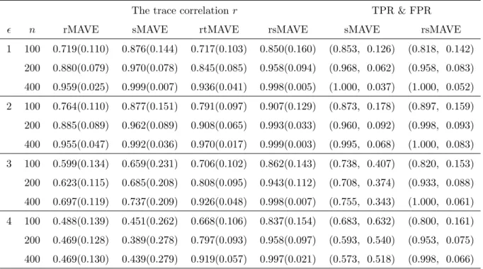
Table 1: Estimation accuracy for independent predictors
The trace correlation𝑟 TPR & FPR
𝜖 𝑛 rMAVE sMAVE rtMAVE rsMAVE sMAVE rsMAVE
1 100 0.719(0.110) 0.876(0.144) 0.717(0.103) 0.850(0.160) (0.853, 0.126) (0.818, 0.142) 200 0.880(0.079) 0.970(0.078) 0.845(0.085) 0.958(0.094) (0.968, 0.062) (0.958, 0.083) 400 0.959(0.025) 0.999(0.007) 0.936(0.041) 0.998(0.005) (1.000, 0.037) (1.000, 0.052) 2 100 0.764(0.110) 0.877(0.151) 0.791(0.097) 0.907(0.129) (0.873, 0.178) (0.897, 0.159) 200 0.885(0.089) 0.962(0.089) 0.908(0.065) 0.993(0.033) (0.960, 0.092) (0.998, 0.093) 400 0.955(0.047) 0.992(0.036) 0.970(0.017) 0.999(0.003) (0.995, 0.068) (1.000, 0.083) 3 100 0.599(0.134) 0.659(0.231) 0.706(0.102) 0.862(0.143) (0.738, 0.407) (0.820, 0.153) 200 0.623(0.115) 0.685(0.208) 0.808(0.095) 0.943(0.112) (0.708, 0.374) (0.933, 0.088) 400 0.697(0.119) 0.737(0.209) 0.926(0.048) 0.998(0.007) (0.755, 0.343) (1.000, 0.061) 4 100 0.488(0.139) 0.451(0.262) 0.668(0.106) 0.837(0.154) (0.683, 0.632) (0.800, 0.161) 200 0.469(0.128) 0.389(0.278) 0.797(0.093) 0.958(0.097) (0.593, 0.540) (0.953, 0.075) 400 0.469(0.130) 0.439(0.279) 0.919(0.057) 0.997(0.021) (0.573, 0.518) (0.998, 0.066)
From the summary of all four different error distributions, we have the following findings. 1. For the standard normal errors, the robust estimation procedures gave comparable results as the least squares based methods, i.e., rtMAVE performed similar to rMAVE
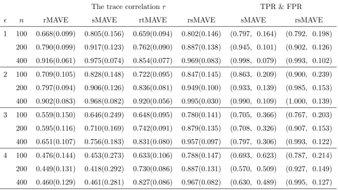
Table 2: Estimation accuracy for correlated predictors
The trace correlation𝑟 TPR & FPR
𝜖 𝑛 rMAVE sMAVE rtMAVE rsMAVE sMAVE rsMAVE
1 100 0.668(0.099) 0.805(0.156) 0.659(0.094) 0.802(0.146) (0.797, 0.164) (0.792, 0.198) 200 0.790(0.099) 0.917(0.123) 0.762(0.090) 0.887(0.138) (0.945, 0.101) (0.902, 0.126) 400 0.916(0.061) 0.975(0.074) 0.854(0.077) 0.969(0.083) (0.998, 0.079) (0.993, 0.102) 2 100 0.709(0.105) 0.828(0.148) 0.722(0.095) 0.847(0.145) (0.863, 0.209) (0.900, 0.239) 200 0.797(0.094) 0.906(0.126) 0.836(0.081) 0.949(0.100) (0.933, 0.139) (0.985, 0.153) 400 0.902(0.083) 0.968(0.082) 0.920(0.056) 0.995(0.030) (0.990, 0.109) (1.000, 0.139) 3 100 0.559(0.150) 0.646(0.249) 0.648(0.095) 0.780(0.141) (0.705, 0.366) (0.767, 0.203) 200 0.595(0.116) 0.710(0.169) 0.742(0.091) 0.879(0.135) (0.708, 0.326) (0.907, 0.153) 400 0.651(0.107) 0.756(0.183) 0.831(0.080) 0.957(0.097) (0.797, 0.306) (0.993, 0.122) 4 100 0.476(0.144) 0.453(0.273) 0.633(0.106) 0.788(0.147) (0.693, 0.623) (0.787, 0.214) 200 0.449(0.131) 0.418(0.292) 0.730(0.086) 0.887(0.131) (0.570, 0.509) (0.927, 0.149) 400 0.460(0.129) 0.461(0.281) 0.827(0.086) 0.967(0.082) (0.630, 0.489) (0.995, 0.127)
and rsMAVE performed similar to sMAVE. In addition, we can see that the sMAVE and rsMAVE achieved better accuracy than rMAVE and rtMAVE respectively due to the sparsity of the model.
2. The MAVE did show some robustness when the errors were from the scaled t-distribution, as mentioned in the original MAVE paper. But with the inclusion of larger outliers in the response as in the error distributions 3 and 4, the least squares based methods failed to estimate the true directions and to select the informative covariates.
3. In the error distributions 2 to 4, the robust estimation procedures performed almost equally well as they did in the cases without outliers. By selecting the informative covariates, the rsMAVE outperformed the rtMAVE in terms of estimation accuracy and also eased the subsequent model building. In addition, rsMAVE also outperformed sMAVE, especially in the error distributions 3 and 4 where some large outliers appear. Based on the above observations, we can conclude that the proposed rsMAVE procedure provided very consistent estimates with good direction estimation and variable selection accuracy in all error distributions considered and had overall best performance among all
four methods considered.
4.2. Estimation of the structural dimension 𝑑
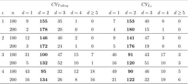
In this section, we evaluate the finite-sample performance of our proposed robust CV procedure based on Tukey’s bisquare loss function for the estimation of dimension 𝑑. Data were generated in the same manner as in model (10). Therefore, the true value of 𝑑 is 2. Here we report only the results from the independent predictors with sample size 𝑛=100 and 200. For each case, 200 data replicates were used. Table 3 summarizes the frequency of estimated 𝑑 out of 200 data replicates. For comparison, the results from𝐿1-based CV were
also reported. We can see that the proposed robust CV procedure provided very consistent estimation for different error distributions. The method performed reasonably well for the cases with outliers, although slightly worse than those without outliers. The robust CV based on Tukey’s bisquare function slightly outperforms the 𝐿1-based CV for distribution 3
and 4, where extreme outliers occur. This can be explained from the influence function where the bisquare function suppresses all the extreme outliers, while the 𝐿1 puts less weights on
them.
Table 3: Frequency of estimated𝑑out of 200 data replicates
𝐶𝑉𝑇 𝑢𝑘𝑒𝑦 𝐶𝑉𝐿1 𝜖 𝑛 𝑑= 1 𝑑= 2 𝑑= 3 𝑑= 4 𝑑≥5 𝑑= 1 𝑑= 2 𝑑= 3 𝑑= 4 𝑑≥5 1 100 9 155 35 1 0 7 153 40 0 0 200 2 178 20 0 0 4 180 15 1 0 2 100 12 146 40 2 0 9 141 47 3 0 200 3 172 24 1 0 5 176 19 0 0 3 100 31 100 47 15 7 46 91 43 17 3 200 5 132 52 10 1 16 120 51 10 3 4 100 43 95 32 12 18 49 90 46 10 5 200 16 134 26 8 16 21 122 32 19 6
5. Logo design data
Wang and Yin (2008) studied a logo design data collected by Henderson and Cote (1998). The objective is to understand how logo design characteristics may influence consumers’ reactions to logos. There are 195 observations and 22 predictors in the data, and the response variable 𝑦 is the logo effect, which ranges from -2.55 to 2.16 with variance around 1. Sparse MAVE (sMAVE; Wang and Yin, 2008) identified 1 significant direction with 9 informative variables out of the 22 as listed in Table 4.
To verify our robust variable selection procedure, we re-analyzed this data set by in-cluding some outliers in the response variable. Two cases were considered in the analysis, a single outlier and 5% contaminated observations. For each case, the outliers were randomly generated by increasing the value𝑦𝑖to𝑦𝑖+𝑐and the results from𝑐=10 and 20 were reported.
From our numerical experience, the pattern were very consistent over different repetitions. In Table 4, we compared the variable selection performance of sMAVE and rsMAVE. To evaluate the estimation accuracy, the correlation between each estimated direction and the directions from sMAVE without outliers, denoted by 𝑐𝑜𝑟𝑟( ˆ𝛽,𝛽ˆ𝑠0), was also presented.
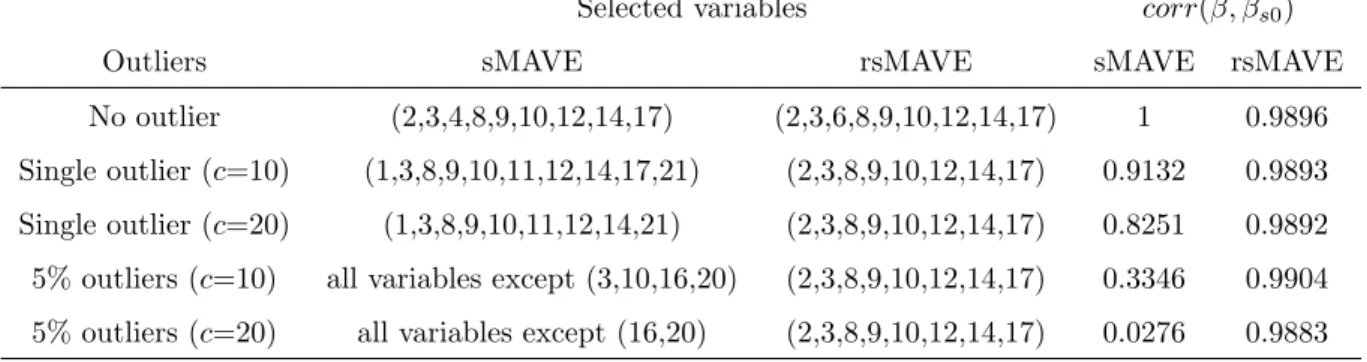
Table 4: Comparison of variable selection. The last column reports the correlations between each estimated directions and the directions from sMAVE without outliers.
Selected variables 𝑐𝑜𝑟𝑟( ˆ𝛽,𝛽ˆ𝑠0)
Outliers sMAVE rsMAVE sMAVE rsMAVE
No outlier (2,3,4,8,9,10,12,14,17) (2,3,6,8,9,10,12,14,17) 1 0.9896 Single outlier (𝑐=10) (1,3,8,9,10,11,12,14,17,21) (2,3,8,9,10,12,14,17) 0.9132 0.9893 Single outlier (𝑐=20) (1,3,8,9,10,11,12,14,21) (2,3,8,9,10,12,14,17) 0.8251 0.9892 5% outliers (𝑐=10) all variables except (3,10,16,20) (2,3,8,9,10,12,14,17) 0.3346 0.9904 5% outliers (𝑐=20) all variables except (16,20) (2,3,8,9,10,12,14,17) 0.0276 0.9883
From the summary, we can see that the performance of sMAVE and rsMAVE are very similar for the original data. After adding outliers, sMAVE is clearly affected in both direction estimation and variable selection. But rsMAVE gives very consistent results, even with 5% extreme values.
6. Conclusion
In this article, we proposed a robust model-free variable selection method, rsMAVE, which combines the strength of both robust and shrinkage estimation. Our numerical studies demonstrate that the proposed method has better performance than the traditional refined MAVE (rMAVE), the sparse MAVE (sMAVE), and the robust MAVE (rtMAVE) when the model is sparse and outliers exist in the response variables. In addition, a robust cross-validation criterion based on Tukey’s bisquare loss function was proposed to select the structural dimension 𝑑.
We believe that this robust variable selection idea can also be extended to models where the response takes discrete values, such as in logistic regression and Poisson regression. The investigation for such a general class is under way.
Acknowledgments
The authors are grateful to Professors P.A. Naik and C.L. Tsai for providing us the Logo design data. The authors would like to thank the Editor, an Associate Editor, and three anonymous referees for their valuable comments and suggestions, which led to substantial improvements in the manuscript.
References
Bellman, R. E. (1961).Adaptive Control Processes. Princeton University Press, Princeton, NJ.
Bondell, H.D. and Li, L. (2008). Shrinkage inverse regression estimation for model free variable selection. Journal of Royal Statistical Society B, 71, 287-299.
Breiman, L. (1995). Better subset regression using the nonnegative Garrote.Technometrics, 37, 373-384. Breiman, L. (1996). Heuristics of instability and stabilization in model selection. Annals of Statistics, 24,
2350–2383. ˇ
C´ıˇzek, P. and H¨𝑎rdle, W. (2006). Robust estimation of dimension reduction space.Computational Statistics and Data Analysis, 51, 545-555.
Cook, R. D. (1998).Regression Graphics: Ideas for studying regressions through graphics. Wiley, New York. Cook, R. D. (2004). Testing predictor contributions in sufficient dimension reduction.Annals of Statistics,
Efron, B., Hasti, T., Johnstone, I. and Tibshirani, R. (2004). Least angle regression.Annals of Statistics, 32, 407–499.
Fan, J. and Jiang, J., (1999). Variable bandwidth and one-step local M-estimator.Science China Series A, 43, 65-81.
Fan, J. and Li, R. (2001). Variable selection via nonconcave penalized likelihood and its oracle properties. Journal of the American Statistical Association, 96, 1348–1360.
Fan, J. and Li, R. (2006). Statistical challenges with high dimensionality: feature selection in knowledge discovery.Proceedings of the international congress of mathematicians, Spain, 2006.
Friedman. J., Hastie, T. and Tibshirani, R. (2010). Regularization paths for generalized linear models via coordinate descent, Journal of Statistical Software, 33, 1–22.
Hampel, F. R., Ronchetti, E. M., Rousseeuw, P. J. and Stahel, W. A. (1986).Robust Statistics: The Approach Based on Influence Functions, Wiley, New York.
Henderson, P. W. and Cote, J. A. (1998). Guidelines for selecting or modifying logos.Journal of Marketing, 62(April), 14–30.
Huber, P. J. (1981).Robust Statistics. Wiley, New York.
Li, K. C. (1991). Sliced inverse regression for dimension reduction (with discussion).Journal of the American Statistical Association, 86, 316–342.
Li, L. (2007). Sparse sufficient dimension reduction.Biometrika, 94, 603–613.
Li, L., Cook, R. D. and Nachtsheim, C. J. (2005). Model-free variable selection.Journal of Royal Statistical Society B, 67, 285–299.
Li, L. and Nachtsheim, C. J. (2006). Sparse sliced inverse regression,Technometrics, 48, 503–510.
Maronna, R. A., Martin, R. D. and Yohai, V. J. (2006).Robust Statistics: Theory and Methods. Wiley, New York.
Ni, L., Cook, R. D. and Tsai, C. L. (2005). A note on shrinkage sliced inverse regression. Biometrika, 92, 242–247.
Rousseeuw, P. J. and Leroy, A. M. (2003).Robust regression and outlier detection, Wiley, New York. Tibshirani, R. (1996). Regression shrinkage and selection via the lasso.Journal of Royal Statistical Society
B, 58, 267–288.
Wang, Q. and Yin, X. (2008). A nonlinear multi-dimensional variable selection method for high dimensional data: Sparse MAVE.Computational Statistics and Data Analysis, 52, 4512-4520.
Wang, Y., Lin, X., Zhu, M. and Bai, Z. (2007). Robust estimation using the Huber function with a data-dependent tuning constant.Journal of Computational and Graphical Statistics, 16, 468-481.
Welsh, A.H. and Ronchetti, E. (2002). A journey in single steps: robust one-step M- estimation in linear regression. Journal of Statistical Planning and Inference, 103, 287-310.
Xia, Y., Tong, H., Li, W. and Zhu, L. (2002). An adaptive estimation of dimension reduction space.Journal of Royal Statistical Society B, 64, 363-410.
Ye, Z. and Weiss, R. E. (2003). Using the bootstrap to select one of a new class of dimension reduction methods. Journal of the American Statistical Association, 98, 968–979.
Zhou, J. and He, X. (2008). Dimension reduction based on constrained canonical correlation and variable filtering.Annals of Statistics, 36, 1649 - 1668.
Zhu, Y. and Zeng, P. (2006). Fourier methods for estimating the central subspace and the central mean subspace in regression. Journal of the American Statistical Association, 101, 1638–1651.
Zou, H. and Hastie, T. (2005). Regularization and variable selection via the elastic net.Journal of Royal Statistical Society B, 67, 301–320.